An Improved Robust Multibasin Profiling Framework with Physics-Protected Selective Structured-Residual Refinement for Thin-Film Thickness Inversion

Abstract

Recovering thin-film thickness from reflectance spectra becomes unreliable when measurements contain sparse outliers, competing thickness minima, or structured mismatch with the nominal optical model. We use a robust multibasin framework in which a Tukey profile first establishes a thickness anchor. A local structured-residual correction is then allowed only in directions that do not reproduce the main thickness-sensitive spectral variation. First-order sensitivity is protected explicitly, and second-order protection is adjusted with an observation-specific curvature-overlap coefficient $C_2$. A frozen gate decides whether the refined candidate replaces the anchor; otherwise, the anchor is returned unchanged. The method was tested in an independent-seed numerical study with 7200 observations spanning three optical systems, three thicknesses, and four contamination conditions. Unprotected residual flexibility did not improve accuracy, whereas adaptive protection reduced the pre-gating mean absolute error to 0.216601 nm. Selective gating reduced harmful accepted refinements from 923 to 495 while retaining 93.28% of beneficial refinements. We then applied the frozen procedure, without experiment-specific retuning, to five physical SiO₂/Si specimens measured at three spatial positions each. Relative to independent model-based ellipsometric references, the specimen-level mean absolute error was 0.374 nm, with relative errors of 0.01–0.15% and within-specimen spatial SDs of 0.16–0.34 nm. These results show that structured residual correction can improve thickness recovery when thickness-sensitive directions are protected and refinement is not forced on every spectrum.

1. Introduction

Thin-film thickness is a key parameter in optical coatings, semiconductor structures, photonic devices, and functional-film fabrication because it directly affects optical phase and interference. Optical methods are attractive for thickness characterization because they are non-contact and can be incorporated into laboratory or process-monitoring workflows. Interferometric, reflectance-based, and ellipsometric approaches have therefore been developed for a range of thin-film measurement tasks [1,2,3,4,5]. In reflectance spectroscopy, however, thickness is not observed directly. It must be inferred through a nonlinear optical model that also depends on material dispersion, substrate response, illumination geometry, and instrumental effects. Recent reflectometry studies further show that angular distribution, spectral bandwidth, calibration, and measurement-model effects can materially influence quantitative thickness recovery [6,7].

Even a nominally simple single-layer inverse problem can contain competing thickness minima over a finite spectral interval, and nuisance terms such as gain or baseline drift can alter the objective landscape. Global, hybrid, and evolutionary searches have been used to reduce dependence on initialization and to explore competing solutions [4,8,9], while physics-constrained spectral strategies target convergence failures over broad thickness ranges [10]. Learning-based estimators provide another route to rapid inversion [11,12,13,14]. These approaches improve search, observability, or direct prediction, but they do not by themselves determine how extra residual flexibility should interact with the spectral directions that identify thickness.

A related problem appears when the nominal forward model does not fully explain the measured spectrum. Sparse high-amplitude deviations can dominate least-squares fitting, motivating robust M-estimation and robust variable-projection methods [15,16]. Smooth discrepancy is different and may arise from background variation, roughness, calibration drift, imperfect optical constants, or optical pathways that are absent from the nominal model [17,18,19]. Adding a flexible residual term can improve spectral agreement, yet that improvement need not translate into a better thickness estimate. If the correction overlaps with directions along which the modeled spectrum changes with thickness, part of the thickness information can be absorbed by the residual model itself. A lower spectral residual can therefore coexist with a worse thickness estimate. This distinction motivates the need to control not only how residual flexibility is introduced but also whether a refined candidate should be allowed to replace the original thickness estimate.

The framework developed here is built around that distinction. A Tukey-based multibasin profile first re-estimates gain and baseline nuisance terms inside the robust objective and refines every finite thickness minimum detected on the deterministic global profile. The selected solution is treated as a data-derived robust anchor. Structured residual flexibility is then introduced only in a local space protected against thickness-sensitive directions. First-order sensitivity is removed explicitly, while second-order protection is adjusted for each observation through the curvature-overlap coefficient $C_2$. Candidate generation and candidate acceptance are kept separate: a local solution may replace the anchor only when prespecified basin, information, structural, and numerical diagnostics are satisfied; otherwise, the anchor is returned unchanged. Projection-based nuisance suppression has a long history in spectral analysis [20,21], but here projection is used specifically to protect the local physical directions that carry thickness information before structured residual correction is admitted. The methodological contribution therefore lies not in any one of these ingredients individually but in their coordinated use to protect thickness-sensitive information and to make residual refinement conditional rather than automatic. In simple terms, the method first obtains a robust global thickness anchor. Local residual correction is then optional: a candidate replaces the anchor only when the frozen diagnostics allow the update; otherwise, the anchor is kept.

The simulations are used to examine the mechanism, and the physical-film experiment tests the frozen pipeline on measured spectra. Numerical evaluation includes mechanism-specific tests, a 7200-observation independent-seed validation across three optical systems, three thicknesses, and four contamination conditions, protection ablations, $C_2$-dependent analyses, selective-gating diagnostics, and a secondary controlled comparator analysis. After the numerical procedure was fixed, the same inversion pipeline was applied without experiment-specific retuning to five physical SiO₂/Si specimens with independent model-based ellipsometric reference thicknesses from 381.74 to 678.67 nm and reflectance measurements at three spatial positions per specimen. The five-specimen SiO₂/Si experiment provides the physical evaluation, while Systems A and C provide complementary numerical tests across different optical configurations.

2. Materials and Methods

2.1. Physics-Based Forward Model and Shared Nuisance Formulation

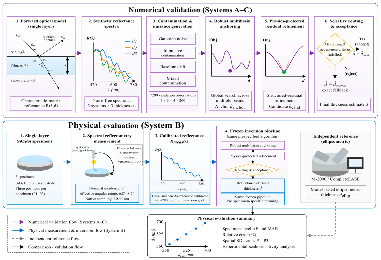
The overall measurement-to-inversion workflow is organized into three stages: reflectance acquisition, robust multibasin anchoring, and physics-protected refinement with selective routing. Figure 1 summarizes this high-level procedure.

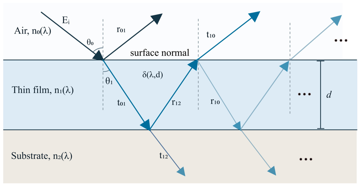
With the overall workflow established, we next define the physical forward model shared by the anchoring and refinement stages. The single-layer reflection geometry is illustrated in Figure 2. The measured spectrum arises from interference between fields reflected at the air–film and film–substrate interfaces, with the phase response governed by wavelength-dependent optical constants, incidence geometry, and film thickness $\mathit{d}$. For numerical Systems A and C, the transparent substrate is represented by a semi-infinite-substrate model.

For wavelength samples ${\lambda }_i$, measured spectrum $y$, candidate thickness $d$, and material/instrument configuration $M$, the forward spectrum $f\left(d;M\right)$ is computed with a coherent single-layer characteristic matrix. For $q\in s,p$,

$$M_q\left(d,\lambda \right)=\left[\begin{array}{cc}\cos \delta & {\displaystyle \frac{i\sin \delta }{{\eta }_{1,q}}}\\ i{\eta }_{1,q}\sin \delta & \cos \delta \end{array}\right],\hspace{1em}\hspace{1em}q\in \left\{s,p\right\},$$

(1)

$$\delta \left(\lambda ,d\right)={\displaystyle \frac{2\pi n_1\left(\lambda \right)d{\cos \theta }_1}{\lambda }},$$

(2)

with ${\eta }_{j,s}=n_j{\cos \theta }_j$ and ${\eta }_{j,p}={\displaystyle \frac{n_j}{{\cos \theta }_j}}, j=0,1,2$. If $M_q=\left[\left[M_{11},M_{12}\right],\left[M_{21},M_{22}\right]\right]$, the amplitude reflection coefficient is

$$r_q={\displaystyle \frac{{\eta }_{0,q}{M}_{11}+{\eta }_{0,q}{\eta }_{2,q}{M}_{12}-M_{21}-{\eta }_{2,q}{M}_{22}}{{\eta }_{0,q}{M}_{11}+{\eta }_{0,q}{\eta }_{2,q}{M}_{12}+M_{21}+{\eta }_{2,q}{M}_{22}}},$$

and unpolarized reflectance is

$$R\left(\lambda ,d\right)={\displaystyle \frac{{\left|r_s\right|}^2+{\left|r_p\right|}^2}{2}}.$$

(3)

Transparent optical constants use the three-term Sellmeier relation

$$n^2\left(\lambda \right)=1+{\displaystyle \sum _{j=1}^3}{\displaystyle \frac{B_j{\lambda }^2}{{\lambda }^2-C_j}},$$

(4)

with fused-silica [22] and N-BK7 [23] coefficients. The SiO₂/Si system uses fixed wavelength-dependent optical constants evaluated on the inversion grid. The SiO₂ entry follows the Malitson dispersion source [22], whereas crystalline-Si optical constants were taken from the KLA/Filmetrics database, whose source record cites Palik [24,25]. The SiO₂-buffer/soda-lime system uses the optical-property data of Aulika et al. and the associated Zenodo dataset [26,27]. In System C, “SiO₂ buffer” denotes the SiO₂ layer on the soda-lime glass substrate. For $\epsilon ={\epsilon }_1+i{\epsilon }_2$,

$$\left|\epsilon \right|=\sqrt{{\epsilon }_1^2+{\epsilon }_2^2},\hspace{1em}\hspace{1em}n=\sqrt{{\displaystyle \frac{\left|\epsilon \right|+{\epsilon }_1}{2}}},\hspace{1em}\hspace{1em}k=\sqrt{{\displaystyle \frac{\left|\epsilon \right|-{\epsilon }_1}{2}}},\hspace{1em}k\ge 0.$$

(5)

The simulations use 361 wavelengths from 420 to 780 nm, incidence angle 8°, and Gaussian spectral blur σ = 0.6 nm. Here, the synthetic spectral blur is implemented by convolving the deterministic spectrum with a Gaussian kernel; on the 1 nm simulation grid, $\sigma =0.6 \mathrm{n}\mathrm{m}$ corresponds to 0.6 samples. This synthetic blur is distinct from the approximately 4.8 nm-FWHM instrumental response used for the physical measurements.

All reference-profile and robust-anchor comparisons use

$$y=gf\left(d;M\right)+B_2\beta +\epsilon ,$$

(6)

Here, $B_2=\left[P_0\left(x\right),P_1\left(x\right),P_2\left(x\right)\right]$ denotes the second-order Legendre baseline basis on the normalized wavelength coordinate $x\in \left[-1, 1\right]$. The coordinate is defined as

$$x\left(\lambda \right)=2{\displaystyle \frac{\lambda -{\lambda }_{\mathrm{m}\mathrm{i}\mathrm{n}}}{{\lambda }_{\mathrm{m}\mathrm{a}\mathrm{x}}-{\lambda }_{\mathrm{m}\mathrm{i}\mathrm{n}}}}-1,$$

which maps the wavelength interval to $x\in \left[-1, 1\right]$. For the 420–780 nm grid used here, this reduces to

$$x\left(\lambda \right)={\displaystyle \frac{\lambda -600}{180}}.$$

The gain is constrained to $0\le g\le 2$. The baseline coefficients are unbounded. Conditional nuisance profiling separates the nonlinear thickness variable from gain and baseline parameters, related in spirit to separable nonlinear least squares and variable projection [16,28,29].

2.2. Constrained L2, Tukey Scoring, and Improved Robust Multibasin Profiling

2.2.1. Observation-Level Robust Scale and Tukey Loss

A single residual scale is estimated for each observation and held fixed across the Tukey-score and robust-anchor thickness evaluations. The complete constrained-L2 profile first yields $d_{L2}$; gain and baseline are refitted there to obtain $r_{\mathrm{p}\mathrm{r}\mathrm{e}}$.

$$s_{\mathrm{M}\mathrm{A}\mathrm{D}}=1.4826\hspace{0.17em}{\mathrm{median}}_i\left|r_{\mathrm{p}\mathrm{r}\mathrm{e},i}-\mathrm{median}\left(r_{\mathrm{p}\mathrm{r}\mathrm{e}}\right)\right|.$$

(7)

The factor 1.4826 provides the usual normal-consistency correction for the median absolute deviation.

If this value is nonfinite or below ${10}^{-6}$, a centered-RMS fallback with the same floor is used. For the scaled residual $u=r/s$ and the fixed Tukey cutoff $c_T=4.685$, the Tukey bisquare loss ${\rho }_T\left(u\right)$ is

$${\rho }_T\left(u\right)=\left\{\begin{array}{cc}{\displaystyle \frac{c_T^2}{6}}\left[1-{\left(1-{\left({\displaystyle \frac{u}{c_T}}\right)}^2\right)}^3\right],& \left|u\right|\le c_T,\\ {\displaystyle \frac{c_T^2}{6}},& \left|u\right|>c_T.\end{array}\right.$$

(8)

The exact Tukey objective is used for selection; the small numerical IRLS weight floor is only a linear-solve safeguard (Supplementary Section S2).

2.2.2. Reference Profiles and Improved Robust Multibasin Anchor

The bounded least-squares reference is

$$J_{\mathrm{L}\mathrm{S}}\left(d\right)=\underset{0\le g\le 2,\beta }{\min }{\displaystyle \frac{1}{n}}{\Vert y-gf\left(d;M\right)-B_2\beta \Vert }_2^2.$$

(9)

The Tukey-score comparator keeps the bounded least-squares nuisance estimate at each d and changes only the residual score:

$$J_{\mathrm{T}\mathrm{S}}\left(d\right)={\displaystyle \frac{1}{n}}\sum _i{\rho }_T\left({\displaystyle \frac{y_i-g_{\mathrm{L}2}\left(d\right)f_i\left(d;M\right)-{\left[B_2{\beta }_{\mathrm{L}2}\left(d\right)\right]}_i}{s}}\right).$$

(10)

The robust multibasin anchor re-estimates the complete nuisance block inside the Tukey profile:

$$J_{\mathrm{r}\mathrm{o}\mathrm{b}}\left(d\right)=\underset{0\le g\le 2,\beta }{\min }{\displaystyle \frac{1}{n}}\sum _i{\rho }_T\left({\displaystyle \frac{y_i-g{f}_i\left(d;M\right)-{\left[B_2\beta \right]}_i}{s}}\right).$$

(11)

The improved robust multibasin anchor uses bounded IRLS, global thickness bounds of 350–700 nm, a 5 nm coarse profile grid, and deterministic gain starts. The coarse grid is used to discover candidate basins over the full thickness interval; it does not set the final thickness resolution, because every finite discrete local-minimum plateau detected on the profile is subsequently refined locally. No fixed top-k truncation is used. Exact numerical tolerances, gain-start values, and candidate-deduplication rules are reported in Supplementary Section S2. This deterministic profile-and-refine strategy provides reproducible multibasin coverage without relying on a stochastic population search and supplies the primary thickness anchor for the protected-refinement stage. The resulting anchor is therefore data-derived from the observed spectrum rather than a predefined initial thickness. The estimator definitions, reader-facing names, and scientific roles are summarized in Table 1.

Table 1. Estimator definitions, reader-facing names, and scientific roles. Core algorithmic settings are summarized in Section 2.3.2, Section 2.3.3 and Section 2.3.4; implementation-level diagnostics and secondary numerical tolerances are provided in the Supplementary Information.

Method	Nuisance Update	Residual Objective	Thickness Search/Routing	Structural Extension	Scientific Role
Bounded least-squares profile	Bounded L2 gain + baseline fit	L2	Bounded thickness profile	None	Coupled L2 reference
Tukey-score profile	Bounded L2 fit; no robust nuisance re-update	Tukey score	Prespecified search	None	Robust-score ablation
Robust multibasin anchor	Bounded robust gain + baseline re-estimation	Tukey	Retained robust-profile minima + deterministic multibasin refinement	None	Primary robust thickness anchor
Proposed method	Anchor-centered local robust refit	Tukey + regularization	Selective local refinement with exact anchor fallback	Thickness-protected residual basis; ${\eta }_2=C_2$	Optional protected refinement with selective gating

Table 1. Estimator definitions, reader-facing names, and scientific roles. Core algorithmic settings are summarized in Section 2.3.2, Section 2.3.3 and Section 2.3.4; implementation-level diagnostics and secondary numerical tolerances are provided in the Supplementary Information.

Method	Nuisance Update	Residual Objective	Thickness Search/Routing	Structural Extension	Scientific Role
Bounded least-squares profile	Bounded L2 gain + baseline fit	L2	Bounded thickness profile	None	Coupled L2 reference
Tukey-score profile	Bounded L2 fit; no robust nuisance re-update	Tukey score	Prespecified search	None	Robust-score ablation
Robust multibasin anchor	Bounded robust gain + baseline re-estimation	Tukey	Retained robust-profile minima + deterministic multibasin refinement	None	Primary robust thickness anchor
Proposed method	Anchor-centered local robust refit	Tukey + regularization	Selective local refinement with exact anchor fallback	Thickness-protected residual basis; ${\eta }_2=C_2$	Optional protected refinement with selective gating

2.3. Physics-Protected Structured-Residual Refinement with Selective Gating

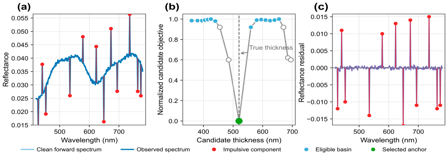
The proposed refinement targets structured residuals that remain after the improved robust multibasin anchor. It operates locally around the anchor, which defines both the expansion point and the exact fallback state. Figure 3 illustrates the anchor-side motivation: sparse contamination can distort the spectrum while the thickness objective contains competing candidate basins, and residual structure may remain after anchor selection. These observations motivate the protected-refinement stage introduced below.

2.3.1. First- and Second-Order Thickness-Sensitivity Protection

Thickness-sensitive directions refer to the local first- and second-order changes of the modeled reflectance spectrum with respect to film thickness after accounting for the shared gain and baseline nuisance space. Let ($d_{\mathrm{a}\mathrm{n}\mathrm{c}\mathrm{h}\mathrm{o}\mathrm{r}}$, $g_{\mathrm{a}\mathrm{n}\mathrm{c}\mathrm{h}\mathrm{o}\mathrm{r}}$, ${\beta }_{\mathrm{a}\mathrm{n}\mathrm{c}\mathrm{h}\mathrm{o}\mathrm{r}}$) denote the thickness, gain, and baseline coefficients of the selected robust-anchor solution, respectively, and let $W_a$ denote its diagonal Tukey-weight matrix. The first-order protected space is

$$T_1=\left[f\left(d_{\mathrm{a}\mathrm{n}\mathrm{c}\mathrm{h}\mathrm{o}\mathrm{r}};M\right), B_2,g_{\mathrm{a}\mathrm{n}\mathrm{c}\mathrm{h}\mathrm{o}\mathrm{r}}{f}^{\prime }\left(d_{\mathrm{a}\mathrm{n}\mathrm{c}\mathrm{h}\mathrm{o}\mathrm{r}};M\right)\right],$$

(12)

with weighted projection

$$P_{T_1,W_a}=T_1{\left(T_1^{\mathsf{T}}{W}_a{T}_1\right)}^{†}{T}_1^{\mathsf{T}}{W}_a.$$

(13)

Here, $†$ denotes the Moore–Penrose pseudoinverse. For later use, ${\Vert v\Vert }_W^2=v^{\mathsf{T}}Wv$, and $P_{S,W}$ denotes the $W$-weighted projector onto the column space of $S$. The symbol ${\epsilon }_{\mathrm{n}\mathrm{u}\mathrm{m}}>0$ denotes a small numerical stabilizer used only in denominator safeguards and is distinct from the spectral residual term $\epsilon$ used in the local model below. The raw multiscale residual dictionary is first residualized:

$$S_1=\left(I-P_{T_1,W_a}\right)S_{\mathrm{r}\mathrm{a}\mathrm{w}}.$$

(14)

Define second-order thickness direction

$$h_2=g_{\mathrm{a}\mathrm{n}\mathrm{c}\mathrm{h}\mathrm{o}\mathrm{r}}{f}^{″}\left(d_{\mathrm{a}\mathrm{n}\mathrm{c}\mathrm{h}\mathrm{o}\mathrm{r}};M\right).$$

(15)

Its component orthogonal to the first-order protected space is

$$h_{2,\perp }=\left(I-P_{T_1,W_a}\right)h_{2.}$$

For vector $v$ and subspace $S$,

$$C\left(v,S;W\right)=1-{\displaystyle \frac{{\Vert W^{1/2}\left(I-P_{S,W}\right)v\Vert }_2^2}{{\Vert W^{1/2}v\Vert }_2^2+{\epsilon }_{\mathrm{n}\mathrm{u}\mathrm{m}}}}.$$

(16)

The observation-specific second-order coherence is

$$C_2=1-{\displaystyle \frac{{\Vert W_a^{1/2}\left(I-P_{S_1,W_a}\right)h_{2,\perp }\Vert }_2^2}{{\Vert W_a^{1/2}{h}_{2,\perp }\Vert }_2^2+{\epsilon }_{\mathrm{n}\mathrm{u}\mathrm{m}}}}.$$

(17)

$${\eta }_2=\mathrm{clip}\left(C_2,0,1\right),$$

(18)

$$S_{\mathrm{p}\mathrm{r}\mathrm{o}\mathrm{t}}=\left(I-{\eta }_2{P}_{2,W_a}\right)S_{1.}$$

(19)

Here $P_{2,W_a}$ denotes the weighted rank-one projector onto the residualized second-order thickness-curvature direction. When this direction is numerically inactive, ${\eta }_2=0$ and the first-order-protected dictionary is retained. Larger $C_2$ means that the residual dictionary can reproduce more of the local second-order thickness direction, so stronger suppression is applied. Because $C_2$ is normalized, ${\eta }_2=C_2$ uses a direct monotone mapping with no additional scalar tuning. Finite-difference and projector details are given in Supplementary Section S3.

2.3.2. Protected Residual Model and Anchor-Centered Local Refinement

The local structured-residual model uses a depth-2 multiscale wavelength tree. Each node contains a smooth local window with constant, linear, and centered quadratic atoms. These atoms represent local offset, slope, and curvature, respectively; the quadratic atom is centered by removing its window-weighted mean. After projection away from the protected thickness-sensitive directions, the surviving atoms form $S_{\mathrm{p}\mathrm{r}\mathrm{o}\mathrm{t}}$. The local model is

$$y=gf\left(d;M\right)+B_2\beta +S_{\mathrm{p}\mathrm{r}\mathrm{o}\mathrm{t}}\gamma +\epsilon .$$

(20)

Candidate refinement minimizes a penalized Tukey objective within an anchor-centered local trust region. The reader-critical settings are a tree depth of 2 with adjacent-window overlap 0.25, regularization coefficients ${\lambda }_{\alpha }=0.05$ and ${\lambda }_{\mathrm{t}\mathrm{r}\mathrm{e}\mathrm{e}}=0.02$, and an anchor-centered trust radius constrained between 2 and 15 nm. The complete objective, secondary numerical safeguards, solver tolerances, and detailed dictionary construction are given in Supplementary Sections S3 and S4.

2.3.3. Selective Refinement Gate

The selective routing layer controls whether a protected local candidate is permitted to replace the robust anchor. Its anchor-level diagnostics use basin separation and local thickness information after gain and baseline adjustment. The operating point was selected on the development registry and frozen before independent validation. Reference thickness is not used at runtime.

Basin separation reflects ambiguity among competing thickness solutions, whereas local information measures how much thickness-sensitive spectral information remains after nuisance adjustment.

Let $J^{\left(1\right)}$ and $J^{\left(2\right)}$ denote the objective values of the two best eligible robust-profile basins, ordered such that $J^{\left(1\right)}\le J^{\left(2\right)}$; the superscripts indicate rank rather than powers. The normalized basin-gap diagnostic is

$$G_{\mathrm{b}\mathrm{a}\mathrm{s}\mathrm{i}\mathrm{n}}={\displaystyle \frac{J^{\left(2\right)}-J^{\left(1\right)}}{\max \left(\left|J^{\left(1\right)}\right|,{\epsilon }_{\mathrm{n}\mathrm{u}\mathrm{m}}\right)}}.$$

If fewer than two eligible basins are found, $J^{\left(2\right)}$ does not exist, and $G_{\mathrm{b}\mathrm{a}\mathrm{s}\mathrm{i}\mathrm{n}}$ is therefore undefined. The implementation records this case as non-finite, so the routing condition fails rather than assigning an artificial basin-gap value. Local thickness information is quantified as the fraction of first-order thickness sensitivity retained after removing the gain and baseline nuisance space:

$$I_{\mathrm{l}\mathrm{o}\mathrm{c}}={\displaystyle \frac{{\Vert \left(I-P_{\left[f\left(d_{\mathrm{a}\mathrm{n}\mathrm{c}\mathrm{h}\mathrm{o}\mathrm{r}};M\right),B_2\right],W_a}\right)g_{\mathrm{a}\mathrm{n}\mathrm{c}\mathrm{h}\mathrm{o}\mathrm{r}}{f}^{\prime }\left(d_{\mathrm{a}\mathrm{n}\mathrm{c}\mathrm{h}\mathrm{o}\mathrm{r}};M\right)\Vert }_{W_a}^2}{{\Vert g_{\mathrm{a}\mathrm{n}\mathrm{c}\mathrm{h}\mathrm{o}\mathrm{r}}{f}^{\prime }\left(d_{\mathrm{a}\mathrm{n}\mathrm{c}\mathrm{h}\mathrm{o}\mathrm{r}};M\right)\Vert }_{W_a}^2+{\epsilon }_{\mathrm{n}\mathrm{u}\mathrm{m}}}}.$$

The selected gate permits protected refinement only when $G_{\mathrm{b}\mathrm{a}\mathrm{s}\mathrm{i}\mathrm{n}}$ is finite with $G_{\mathrm{b}\mathrm{a}\mathrm{s}\mathrm{i}\mathrm{n}}\le 5.0$ and $I_{\mathrm{l}\mathrm{o}\mathrm{c}}\ge 0.82$. These are development-selected operating thresholds rather than physical constants, and they were frozen before independent-seed validation.

2.3.4. Candidate Acceptance and Exact Anchor Fallback

For observations entering protected refinement, the local model generates an anchor-centered candidate. The selective routing rule together with frozen structural, numerical, and candidate-quality safeguards then determines whether the candidate replaces the anchor. If any routing, convergence, or acceptance requirement fails, the robust anchor is returned exactly.

Passing the selective gate permits candidate evaluation but does not guarantee acceptance. The normalized candidate objective improvement is

$$G_A={\displaystyle \frac{J_{\mathrm{a}\mathrm{n}\mathrm{c}\mathrm{h}\mathrm{o}\mathrm{r}}-J_{\mathrm{c}\mathrm{a}\mathrm{n}\mathrm{d}\mathrm{i}\mathrm{d}\mathrm{a}\mathrm{t}\mathrm{e}}}{\max \left(\left|J_{\mathrm{a}\mathrm{n}\mathrm{c}\mathrm{h}\mathrm{o}\mathrm{r}}\right|,{\epsilon }_{\mathrm{n}\mathrm{u}\mathrm{m}}\right)}}.$$

Final acceptance requires a finite and converged candidate strictly inside the local trust interval, fitted gain within $\left[0, 2\right]$, $G_A\ge 5\times {10}^{-4}$, retained first-order information $R_I\ge 0.5$, and second-order leakage $L_2\le 0.25$; secondary robust-consensus and numerical safeguards are reported in Supplementary Section S4.

$$\widehat{d}=\left\{\begin{array}{cc}{d}_{\mathrm{c}\mathrm{a}\mathrm{n}\mathrm{d}},& \mathrm{if} \mathrm{all} \mathrm{frozen} \mathrm{safeguards} \mathrm{are} \mathrm{satisfied},\\ d_{\mathrm{a}\mathrm{n}\mathrm{c}\mathrm{h}\mathrm{o}\mathrm{r}},& \mathrm{otherwise}.\end{array}\right.$$

(21)

Thus, the 4790 validation observations reported as fallbacks return a final thickness numerically identical to the corresponding robust anchor; no partial or approximate update is applied in those cases.

2.4. Numerical Evidence Design

The numerical evaluation comprises a mechanism-specific benchmark, a 7200-observation cross-material study with independent-seed validation, and a secondary controlled comparator analysis. These numerical studies were completed independently of the later physical-film evaluation described in Section 2.5. A synthetic reflectance spectrum is generated from the prescribed forward model at a known generating thickness and is then perturbed according to the specified nuisance and contamination model; the known generating thickness is used only for post-inversion evaluation.

2.4.1. Mechanism Benchmark

A mechanism-specific benchmark on the fused-silica/N-BK7 system was used to characterize the reference profiles under Gaussian, impulsive, baseline-drift, and mixed contamination. The independent statistical unit was the observation, and each contamination family was analyzed separately. Full execution counts and registry details are reported in the Supplementary Information.

2.4.2. Cross-Material Simulation Study

The main simulation study used material systems A = fused silica/N-BK7, B = SiO₂/Si, and C = SiO₂ buffer/soda-lime glass; true thicknesses 380, 520, and 680 nm; and four contamination conditions. Each of the 36 cells contained 200 independent observations (7200 observations; 21,600 bounded-L2/Tukey-score/robust-anchor records). Systems A and C broaden the numerical evaluation across transparent-substrate configurations, while System B connects the numerical study with the five-specimen SiO₂/Si experiment. The optical systems and common numerical-validation settings are summarized in Table 2.

Table 2. Optical systems and common numerical-validation settings.

System	Film	Substrate	Optical-Constant Treatment	True Thicknesses, d (nm)
A	Fused silica	N-BK7	Analytic Sellmeier relations	380, 520, 680
B	SiO2	Si	Frozen wavelength-dependent optical-constant tables	380, 520, 680
C	SiO2 buffer	Soda-lime glass	Frozen ε-to-(n,k) optical-constant data	380, 520, 680

Table 2. Optical systems and common numerical-validation settings.

System	Film	Substrate	Optical-Constant Treatment	True Thicknesses, d (nm)
A	Fused silica	N-BK7	Analytic Sellmeier relations	380, 520, 680
B	SiO2	Si	Frozen wavelength-dependent optical-constant tables	380, 520, 680
C	SiO2 buffer	Soda-lime glass	Frozen ε-to-(n,k) optical-constant data	380, 520, 680

The four prespecified contamination conditions are summarized in

Table 3. Contamination settings used in the numerical validation.

Condition	Gaussian SD	Outliers	Nominal Outlier Magnitude	Baseline Amplitude	Gain SD	Offset SD
Gaussian	0.0008	0	0	0	0.005	0.0002
Impulsive	0.0004	4% (14/361)	0.012	0	0.005	0
Baseline drift	0.0004	0	0	0.0035	0.005	0
Mixed	0.0008	6% (22/361)	0.015	0.0035	0.008	0.0003

.

With $x\in \left[-1, 1\right]$, the contaminated observations were generated as

$$y=gf\left(d_{\mathrm{t}\mathrm{r}\mathrm{u}\mathrm{e}};M\right)+o\mathbf{1}+b\left(x\right)+\epsilon +o_{\mathrm{s}\mathrm{p}\mathrm{a}\mathrm{r}\mathrm{s}\mathrm{e}},$$

(22)

$$b_{\mathrm{r}\mathrm{a}\mathrm{w}}\left(x\right)=c_0+c_{1}x+c_2{x}^2+c_3\sin \left(\omega x+\varphi \right),$$

(23)

where $b_{\mathrm{r}\mathrm{a}\mathrm{w}}\left(x\right)$ defines the smooth structured-drift template, and $\omega$ is a fixed low-frequency simulation factor. The template was normalized and scaled to the condition-specific baseline amplitude to obtain $b\left(x\right).$ The exact value of $\omega$, coefficient and phase distributions, sparse-outlier generation, RNG construction, and registered contamination settings are reported in Supplementary Section S5 and Table S4. The resulting 36-cell design provides a controlled cross-material and cross-thickness test bed for the inversion framework. Impulsive contamination means that a small number of wavelength samples in each simulated spectrum are deliberately assigned large perturbations. For each observation, the affected wavelength indices are drawn uniformly without replacement; perturbation signs are equiprobable $\pm 1$, and magnitudes follow the prespecified contamination distribution. The impulsive condition corrupts 14 of 361 wavelength points (4%), whereas the mixed condition corrupts 22 points (6%).

2.4.3. Refinement Development, Freeze, and Independent-Seed Validation

Only the optional protected-refinement layer and its selective gate were developed after the robust anchor had been fixed. The gate operating point was selected from a prespecified development grid using a risk-first criterion: harmful accepted refinements were minimized subject to retaining at least 90% of the mean-AE benefit provided by ungated protected refinement. The selected thresholds were then frozen together with the refinement architecture and candidate safeguards. Independent validation regenerated 7200 observations under the same 36-cell material–thickness–contamination design using a distinct master seed, with no validation-set retuning. Exact development grids, selected thresholds, RNG construction, and provenance checks are reported in Supplementary Section S5. Here, “master seed” denotes the integer used to initialize pseudorandom-number generation. The development and independent-validation master seeds were 20260426 and 20260508, respectively.

2.4.4. Controlled Comparative Benchmark

A secondary controlled benchmark was used only for algorithmic comparison under a common inversion problem. The benchmark compared the proposed procedure with bounded spectral fitting, multi-start simplex, and genetic-algorithm inversion on the same 144 synthetic spectra using common forward-model assumptions and thickness bounds. It was deliberately restricted to direct inversion methods that do not require a separate training stage. Its design, comparator settings, validity rules, timing protocol, and complete results are reported in Supplementary Sections S6 and S17.

2.5. Physical SiO₂/Si Measurement and Reference Characterization

Five single-layer SiO₂/Si thin-film wafers were used for the physical evaluation, spanning approximately 382–679 nm in reference thickness. Reflectance spectra were acquired using an AvaSpec-VRS2048CL-EVO spectrometer with an MN0300-0.30 grating (300 lines/mm), a 100 μm entrance slit, and an AvaLight-DHc source; both instruments were from Avantes B.V., Apeldoorn, The Netherlands. The configuration had a nominal spectral FWHM of approximately 4.8 nm. Absolute-reflectance calibration using a bare-Si reference followed the general procedure reported by Bai et al. [4], with adaptations to the present fiber-coupled spectrometer and bracketing acquisition sequence. Reference and dark spectra were each averaged over ten acquisitions, following the acquisition structure described by Sánchez-Arriaga et al. [3].

For each specimen, acquisition used the bracketing sequence $D_{before}$ → $R_{before}$ → $P1$/$P2$/$P3$ → $R_{after}$ → $D_{after}$. P1–P3 denote three predefined spatial positions on each specimen, and each position was calibrated and inverted independently. The before/after dark and bare-Si reference spectra were linearly interpolated in acquisition time to each sample-position measurement. For position $k$, $D_k\left(\lambda \right)$ and $I_{\mathrm{S}\mathrm{i},k}\left(\lambda \right)$ therefore denote the time-interpolated dark and bare-Si reference spectra, respectively. Each position was then calibrated independently according to

$$R_k\left(\lambda \right)={\displaystyle \frac{I_k\left(\lambda \right)-D_k\left(\lambda \right)}{I_{\mathrm{S}\mathrm{i},k}\left(\lambda \right)-D_k\left(\lambda \right)}}{R}_{\mathrm{S}\mathrm{i}}\left(\lambda \right),$$

(24)

where $I_k\left(\lambda \right)$ is the measured sample intensity at position $k$, $D_k\left(\lambda \right)$ and $I_{\mathrm{S}\mathrm{i},k}\left(\lambda \right)$ are the corresponding time-interpolated dark and bare-Si reference spectra, and $R_{\mathrm{S}\mathrm{i}}\left(\lambda \right)$ is the theoretical wavelength-dependent reflectance of the bare-Si reference used to convert the measured relative spectrum to absolute reflectance.

Reflectance calibration was completed on the native wavelength axis before resampling. The calibrated native axis contained 819 wavelength samples from 420.274 to 779.922 nm, with a mean sampling interval of approximately 0.4397 nm; this sampling interval is distinct from the approximately 4.8 nm instrumental FWHM. The calibrated spectra were linearly resampled to the fixed 420–780 nm, 1 nm inversion grid, with nearest-value handling at the two terminal points. For a target wavelength $\lambda$ lying between adjacent calibrated native wavelengths ${\lambda }_j$ and ${\lambda }_{j+1}$, linear interpolation was performed as

$$R_{\mathrm{i}\mathrm{n}\mathrm{t}}\left(\lambda \right)=R_j+{\displaystyle \frac{\lambda -{\lambda }_j}{{\lambda }_{j+1}-{\lambda }_j}}\left(R_{j+1}-R_j\right),$$

The approximately 0.44 nm value characterizes the native sampling interval, whereas the 4.8 nm FWHM characterizes the instrumental spectral response; the two quantities therefore enter the processing chain separately.

For the physical measurements, the forward reflectance was angle-averaged according to the implemented probe weighting $p\left(\theta \right)$ over the effective 6.8–8.7° angular range and then convolved with a Gaussian instrumental-response kernel with a FWHM of 4.8 nm before comparison with the resampled spectra.

Independent model-based reference thicknesses were obtained with a J.A. Woollam M-2000 spectroscopic ellipsometer (J.A. Woollam Co., Inc., Lincoln, NE, USA) using CompleteEASE version 6.51. Measurements covered 400–1000 nm at incidence angles of 65°, 70°, and 75°, and the angle-dependent $\Psi \left(\lambda \right)$ and $\Delta \left(\lambda \right)$ spectra were fitted jointly. All five specimens were fitted with an ambient/roughness/SiO₂/Si stack. The roughness layer used a 50% SiO₂/50% void Bruggeman EMA. SiO₂ was represented as a transparent Cauchy layer, $n\left(\lambda \right)=A+B/{\lambda }^2+C/{\lambda }^4$, with $\lambda$ expressed in μm and $k=0$; thickness and Cauchy $A$ and $B$ were fitted, with $C$ fixed at zero. The reported ellipsometric film thickness corresponds to the fitted dense SiO₂ layer, while the EMA roughness-layer thickness was treated as a separate fitted parameter. Crystalline-Si optical constants were taken from the CompleteEASE database.

The ellipsometer measured the same three nominal specimen regions (P1–P3) used for reflectance characterization. The reported reference is the mean of the three position-specific thickness fits, with SD across those three positions. The reflectance inversion retained its prespecified nominal optical-constant model; specimen-specific ellipsometric dispersion estimates were reserved for independent characterization and post hoc sensitivity analysis. The inversion architecture and all decision rules were fixed before the physical measurements and were not retuned to these specimens. The specimen is therefore the experimental unit (n = 5), with three nested spatial measurements per specimen. The key reflectance and ellipsometric settings used in the physical-film study are summarized in Table 4.

Table 4. Key reflectance and ellipsometric settings used in the physical-film study.

Item	Setting
Specimens	Five single-layer SiO2/Si films
Spectrometer	AvaSpec-VRS2048CL-EVO
Light source	AvaLight-DHc
Spectral configuration	MN0300-0.30 grating, 300 lines/mm; 100 μm entrance slit
Instrumental response	Gaussian, nominal FWHM ≈ 4.8 nm
Measurement geometry	Nominal 8° incidence; modeled effective angular range 6.8–8.7°
Analysis window	420–780 nm; resampled to 1 nm spacing (361 points)
Spectral averaging	10 acquisitions per dark, reference, and sample-position record
Spatial sampling	Three corresponding positions (P1–P3) per specimen; positions processed independently
Reference thickness	J.A. Woollam M-2000 ellipsometry; 400–1000 nm; 65°, 70°, and 75°

Table 4. Key reflectance and ellipsometric settings used in the physical-film study.

Item	Setting
Specimens	Five single-layer SiO2/Si films
Spectrometer	AvaSpec-VRS2048CL-EVO
Light source	AvaLight-DHc
Spectral configuration	MN0300-0.30 grating, 300 lines/mm; 100 μm entrance slit
Instrumental response	Gaussian, nominal FWHM ≈ 4.8 nm
Measurement geometry	Nominal 8° incidence; modeled effective angular range 6.8–8.7°
Analysis window	420–780 nm; resampled to 1 nm spacing (361 points)
Spectral averaging	10 acquisitions per dark, reference, and sample-position record
Spatial sampling	Three corresponding positions (P1–P3) per specimen; positions processed independently
Reference thickness	J.A. Woollam M-2000 ellipsometry; 400–1000 nm; 65°, 70°, and 75°

2.6. Local Model-Parameter and Experimental-Scale Sensitivity Analysis

A separate one-factor-at-a-time sensitivity analysis was performed around the nominal 521.5 nm SiO₂/Si configuration. The SiO₂ refractive-index curve was scaled by −1.0%, −0.5%, 0, +0.5%, and +1.0%; incidence angle was evaluated at 6°, 8°, and 10°; and wavelength offsets of −0.5, 0, and +0.5 nm were applied. Only one factor was varied at a time while the remaining settings were held fixed. These deliberately broad perturbations were used as nominal stress probes for local model sensitivity.

To relate these nominal stress probes to the experimental scales of the five measured specimens, additional one-factor analyses used specimen-specific ellipsometric dispersion, wavelength-calibration, and holder-alignment information.

For each specimen, the Cauchy dispersion obtained independently from the M-2000/CompleteEASE characterization was compared with the nominal Malitson SiO₂ dispersion used in the reflectance inversion over 420–780 nm. The maximum relative dispersion difference, ${\mathrm{m}\mathrm{a}\mathrm{x}}_{\lambda }\mid \mathsf{\Delta }n\left(\lambda \right)/n\left(\lambda \right)\mid$, was recorded to characterize the magnitude of the dispersion mismatch, and the corresponding specimen-specific Cauchy dispersion was then substituted in the one-factor post hoc analysis with the remaining inversion settings held fixed.

Wavelength calibration based on standard spectral lines gave a calibration-error scale of $\pm 0.17$ nm, with a maximum absolute calibration residual of 0.25 nm. Specimen-specific thickness response was therefore evaluated after shifting the calibrated wavelength axis by $\pm 0.17$ nm while retaining the remaining model settings.

The independently established mechanical holder angular tolerance was $\pm {0.3}^{\circ }$. Its effect was evaluated by shifting the complete angular weighting distribution $p\left(\theta \right)$ by $\pm {0.3}^{\circ }$ for each specimen.

Reference-fit stability was characterized by two independent CompleteEASE fits of the same retained M-2000 dataset for each specimen. The resulting fit-to-fit thickness differences provide a separate measure of the stability of the ellipsometric optical-model solution.

The experimental-scale responses are reported separately by factor so that the contributions associated with dispersion, wavelength calibration, angular alignment, and reference-fit stability remain individually interpretable.

2.7. Statistical Estimands and Failure Accounting

Accuracy was summarized with absolute error (AE), mean AE, and q90/q95 AE. Prespecified method comparisons used paired observation-level contrasts, with paired bootstrap confidence intervals for the main mean effects. Exact anchor fallbacks remained in unconditional accounting. For the physical-film evaluation, the specimen was the statistical unit; the three spatial positions were treated as nested measurements. The primary physical-film MAE was calculated from the five unrounded specimen means, while position-level and repeat-fit results were treated as supporting characterization. Detailed estimands, failure accounting, bootstrap rules, and comparator validity definitions are given in the Supplementary Information. For validation only, a refinement candidate was labeled beneficial if it reduced absolute thickness error relative to the anchor and harmful if it increased that error. These labels use the known reference thickness only for post hoc evaluation and are never inputs to the gate.

2.8. Computational Implementation and Provenance

All computations used a frozen Python implementation. RNG, registry-provenance, resampling, and checksum summaries are provided in Supplementary Section S16, and implementation-specific timing is reported in Supplementary Section S15.

The numerical implementation, frozen configuration files, manuscript-aligned numerical summary tables, and verification scripts are publicly available at https://github.com/you-love520/selective-protected-thin-film-inversion (accessed on 30 August 2026).

Timing was evaluated on an Intel Core i7-13700 processor (Intel Corporation, Santa Clara, CA, USA), using Python 3.12 with one worker, one BLAS thread, one performance core, and no GPU after 200 warm-up observations. Five complete passes through the 7200-observation validation registry provided 36,000 spectrum-level executions for the runtime summary.

The reported timing therefore characterizes a serial implementation. Because spectrum-level inversions are independent at the batch level, the workflow is directly amenable to parallel execution across observations.

3. Results

3.1. Robust Multibasin Profiling Under Contamination and Competing Minima

The mechanism benchmark identified the regimes in which robust profiling provides the largest stabilization benefit. Sparse impulsive contamination produced the clearest degradation of the bounded least-squares profile, whereas approximately Gaussian observations showed much smaller differences. Cross-material performance was then evaluated in the independent 7200-observation cross-material study.

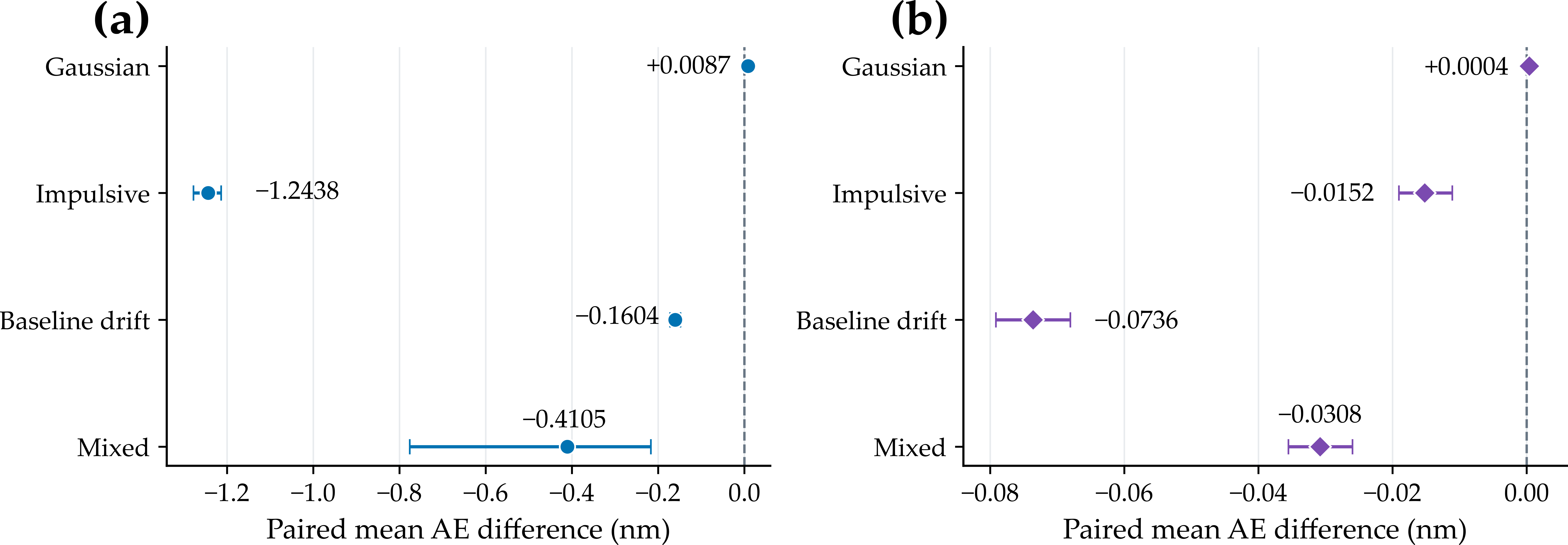
Across the three optical systems and three thicknesses, the robust multibasin anchor showed clear mechanism dependence (Figure 4). Impulsive contamination produced the largest improvement relative to bounded least squares (mean absolute-error difference −1.243760 nm; q95 difference −2.143210 nm). Baseline drift and mixed contamination also favored the anchor. Under Gaussian contamination, the differences were small and slightly favored the reference profiles. The same overall pattern relative to the Tukey-score profile indicates that robust nuisance re-estimation and multibasin profiling matter most under structured or impulsive contamination. Complete mean/q90/q95 contrasts and bootstrap intervals are reported in Supplementary Table S10.

3.2. Refinement Gains Depend on Protecting Thickness-Sensitive Directions

The ablation identifies physical protection—not residual flexibility alone—as the source of refinement gain (

Table 5. Protection and selective-gating ablation across the 7200-observation validation registry. Harmful fraction is conditional on accepted refinements.

Arm	Mean Absolute Error (nm)	Accepted	Improved	Harmed	Harmful Among Accepted
Robust multibasin anchor	0.223465	0	0	0	—
Unprotected residual refinement	0.223613	3287	2017	1270	38.64%
First-order protected refinement	0.217689	3168	2067	1101	34.75%
Fixed full second-order protection	0.226053	3047	1887	1160	38.07%
Adaptive $C_2$ protected refinement	0.216601	2976	2053	923	31.01%
Proposed selective protected refinement	0.194634	2410	1915	495	20.54%

An em dash (—) indicates that the entry is not applicable because no refinements were accepted for the robust multibasin anchor.

). Unprotected residual refinement slightly increased mean absolute error from 0.223465 nm for the robust anchor to 0.223613 nm and harmed 38.64% of accepted candidates. This reverse comparison directly shows that unconstrained residual correction can degrade thickness recovery even when it adds fitting flexibility. First-order protection reduced mean absolute error to 0.217689 nm and the harmful fraction to 34.75%. Fixed full second-order protection increased the mean absolute error to 0.226053 nm, consistent with uniformly imposed second-order suppression being overly restrictive, whereas observation-specific $C_2$ protection yielded the lowest mean absolute error before selective gating, 0.216601 nm.

These results show that useful residual correction depends on where flexibility is allowed to act. First-order protection removes direct overlap with local thickness sensitivity, while $C_2$ adapts second-order suppression to residual-curvature geometry instead of imposing the same curvature constraint on every observation.

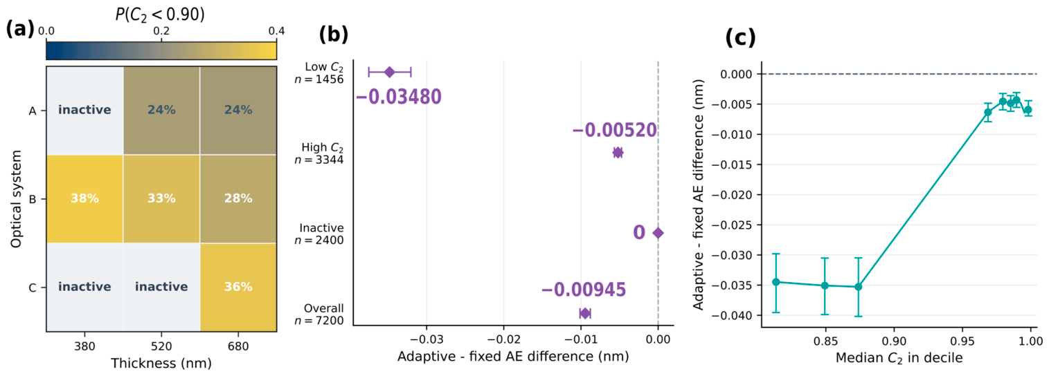
Second-order protection was inactive in 2400 observations and active in 4800. Relative to fixed full protection, adaptive $C_2$ produced a larger mean gain when $C_2$ < 0.90 (−0.034800 nm; 95% CI, −0.037483 to −0.032042 nm) than when $C_2$ ≥ 0.90 (−0.005200 nm; 95% CI, −0.005674 to −0.004745 nm), while inactive cases were identical by construction. The $C_2=0.90$ split is used only for descriptive reporting and is not a routing threshold.

The continuous analysis showed the same low-to-high coherence gradient (Figure 5). Across the 4800 active observations, Spearman rho between $C_2$ and the adaptive-minus-fixed absolute-error difference was +0.1677 (95% CI, +0.1400 to +0.1966); because negative differences favor adaptive protection, the positive association indicates that the adaptive advantage becomes smaller as $C_2$ increases. This pattern is consistent with the intended role of $C_2$ as an observation-specific geometric controller rather than a contamination label.

3.3. Selective Gating Controls Harmful Refinement

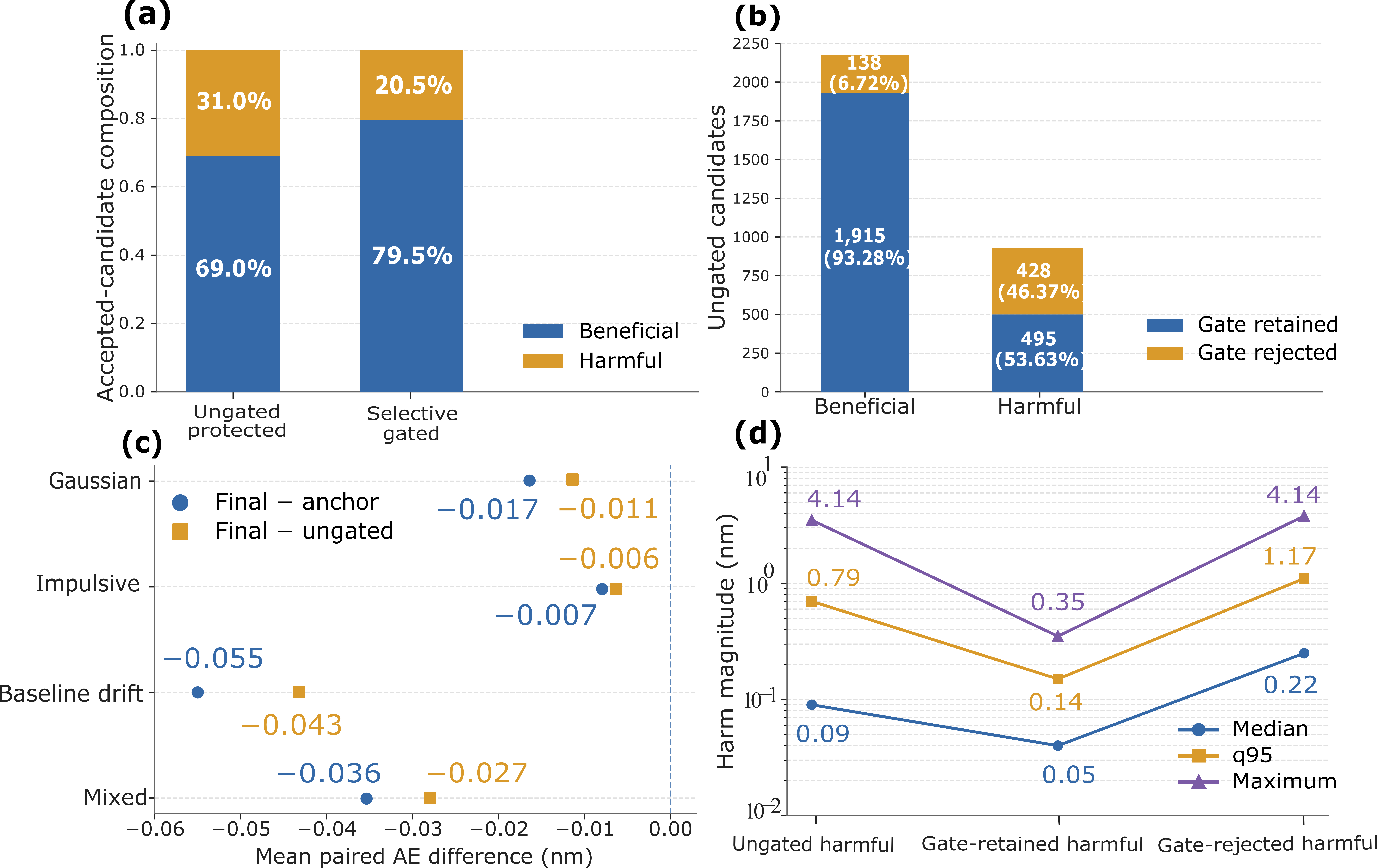
Selective gating controls whether a protected local candidate can replace the anchor. Ungated refinement accepted 2976 candidates (2053 beneficial and 923 harmful); the frozen gate retained 2410 (1915 beneficial and 495 harmful), with the other 4790 observations returning the robust anchor exactly. The gate rejected 46.37% of harmful candidates while retaining 93.28% of beneficial candidates, reducing the harmful fraction among accepted refinements from 31.01% to 20.54%.

Harm severity was also concentrated in the rejected subset (Figure 6). q95 worsening was 0.790287 nm across all ungated harmful refinements, 0.141396 nm among harmful refinements retained by the gate, and 1.176674 nm among rejected harmful refinements. The selective layer therefore reduced both the incidence and the upper-tail severity of harmful intervention.

3.4. Paired Accuracy Gains Persist Across Contamination Scenarios

The resulting benefit is not limited to routing composition: the final estimator also improved pooled mean absolute error relative to ungated protected refinement. Candidate generation and permission to modify the anchor are therefore treated as separate operations. This distinction is especially useful when residual flexibility can improve local spectral fit without necessarily improving the inferred thickness.

Scenario-wise paired mean effects remained favorable in all four prespecified contamination families (Figure 6c). The largest mean gain relative to the anchor occurred under baseline drift (−0.055510 nm), whereas impulsive contamination required the fewest accepted refinements (414 of 1800), leaving 1386 observations at the robust anchor. Complete scenario-wise routing and fallback counts are reported in Supplementary Tables S7 and S8.

3.5. Physical-Film Results

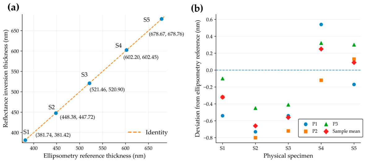
The physical-film evaluation covered five SiO₂/Si specimens with ellipsometric reference thicknesses from 381.74 to 678.67 nm. Three spatial positions (P1–P3) were measured on each specimen. Each reflectance position was independently calibrated and inverted; the three reflectance-derived thicknesses were then summarized by specimen mean and SD across the three positions and compared with the specimen ellipsometric reference.

The specimen-level MAE was 0.374 nm. Individual absolute errors ranged from 0.09 to 0.66 nm, relative errors from 0.01% to 0.15%, and the spatial SD across the three reflectance positions from 0.16 to 0.34 nm. The inversion settings were not retuned for these specimens. The specimen-level agreement and position-level deviations are shown in Figure 7. The corresponding specimen-level thickness results are summarized in Table 6.

Figure 7. Physical-film evaluation of the frozen inversion procedure on five SiO₂/Si specimens. (a) Mean reflectance-derived thickness versus the independent model-based specimen ellipsometric reference; vertical error bars show the spatial SD across the three reflectance positions; at this scale, they are smaller than the plotted symbols. The dashed identity line indicates exact agreement. (b) Position-level deviations from the specimen ellipsometric reference; diamonds show the specimen mean deviation. P1–P3 are nested spatial measurements within each specimen. The spatial SD describes within-specimen spatial variability and should not be interpreted as the total metrological uncertainty of the measurement system. The inversion settings were not retuned for these specimens.

Figure 7. Physical-film evaluation of the frozen inversion procedure on five SiO₂/Si specimens. (a) Mean reflectance-derived thickness versus the independent model-based specimen ellipsometric reference; vertical error bars show the spatial SD across the three reflectance positions; at this scale, they are smaller than the plotted symbols. The dashed identity line indicates exact agreement. (b) Position-level deviations from the specimen ellipsometric reference; diamonds show the specimen mean deviation. P1–P3 are nested spatial measurements within each specimen. The spatial SD describes within-specimen spatial variability and should not be interpreted as the total metrological uncertainty of the measurement system. The inversion settings were not retuned for these specimens.

Table 6. Physical-film thickness evaluation on five SiO₂/Si specimens. The three position columns are spatial measurements on the same specimen; SD is the standard deviation across those positions.

Specimen	P1 (nm)	P2 (nm)	P3 (nm)	Reflectance Mean ± SD (nm)	Ellipsometry Reference (nm)	AE (nm)	Relative Error (%)
S1	381.20	381.42	381.64	381.42 ± 0.22	381.74	0.32	0.08
S2	447.65	447.58	447.93	447.72 ± 0.19	448.38	0.66	0.15
S3	520.92	520.74	521.05	520.90 ± 0.16	521.46	0.56	0.11
S4	602.74	602.08	602.52	602.45 ± 0.34	602.20	0.25	0.04
S5	678.50	678.80	678.97	678.76 ± 0.24	678.67	0.09	0.01

Note: P1–P3 are spatial reflectance measurements on the same specimen. AE = |reflectance mean − ellipsometry reference|. Relative error = AE/reference × 100%. Overall MAE was calculated from the unrounded specimen means.

Table 6. Physical-film thickness evaluation on five SiO₂/Si specimens. The three position columns are spatial measurements on the same specimen; SD is the standard deviation across those positions.

Specimen	P1 (nm)	P2 (nm)	P3 (nm)	Reflectance Mean ± SD (nm)	Ellipsometry Reference (nm)	AE (nm)	Relative Error (%)
S1	381.20	381.42	381.64	381.42 ± 0.22	381.74	0.32	0.08
S2	447.65	447.58	447.93	447.72 ± 0.19	448.38	0.66	0.15
S3	520.92	520.74	521.05	520.90 ± 0.16	521.46	0.56	0.11
S4	602.74	602.08	602.52	602.45 ± 0.34	602.20	0.25	0.04
S5	678.50	678.80	678.97	678.76 ± 0.24	678.67	0.09	0.01

Note: P1–P3 are spatial reflectance measurements on the same specimen. AE = |reflectance mean − ellipsometry reference|. Relative error = AE/reference × 100%. Overall MAE was calculated from the unrounded specimen means.

Independent M-2000/CompleteEASE characterization also provided specimen-specific SiO₂ Cauchy parameters and EMA roughness-layer thicknesses (

Table 7. Specimen-specific M-2000/CompleteEASE characterization used for independent optical-property assessment. Thickness values are means ± SD across the three corresponding ellipsometric positions. The Cauchy model is $n\left(\lambda \right)=A+B/{\lambda }^2$, with $\lambda$ expressed in $\mathsf{\mu }\mathrm{m}$; the roughness layer is the fitted 50% SiO₂/50% void EMA layer.

Specimen	M-2000 Thickness (nm)	Cauchy $\mathit{A}$	Cauchy $\mathit{B}$ (μm2)	EMA Roughness (nm)	Max. |Δn/n| (%)
S1	381.74 ± 0.18	1.4491590	0.003494059	1.744	0.0847
S2	448.38 ± 0.18	1.4485654	0.003595880	1.467	0.0583
S3	521.46 ± 0.29	1.4476501	0.003491001	0.999	0.0494
S4	602.20 ± 0.33	1.4469905	0.003578737	1.114	0.0759
S5	678.67 ± 0.15	1.4488996	0.003513860	1.351	0.0691

). Across the five specimens, the fitted Cauchy coefficient $A$ ranged from 1.4469905 to 1.4491590, while $B$ ranged from 0.003491001 to 0.003595880 $\mathrm{\mu }{\mathrm{m}}^2$. The fitted roughness-layer thickness ranged from 0.999 to 1.744 nm. Relative to the nominal Malitson dispersion used in reflectance inversion, the maximum specimen-specific refractive-index difference over 420–780 nm was 0.0494–0.0847%.

Because the final estimator can retain the anchor unchanged, we also compared the robust-anchor outputs with the final selective estimates from the same frozen physical runs. The anchor-only specimen-level MAE was 0.512 nm, compared with 0.374 nm for the final estimator. Protected refinement was accepted for eight of the 15 position-level spectra, while the remaining seven returned the robust anchor exactly. The anchor was already accurate on this measured set, while selective refinement further reduced the specimen-level error without being applied to every spectrum. The specimen-level comparison is summarized in

Table 8. Robust-anchor-only and final selective thickness estimates for the five physical SiO₂/Si specimens.

Specimen	Ellipsometry Reference (nm)	Robust-Anchor Mean ± SD (nm)	Final Mean ± SD (nm)	Anchor AE (nm)	Final AE (nm)	Accepted Positions
S1	381.74	381.25 ± 0.66	381.42 ± 0.22	0.49	0.32	2/3
S2	448.38	447.58 ± 0.56	447.72 ± 0.19	0.80	0.66	2/3
S3	521.46	520.83 ± 0.28	520.90 ± 0.16	0.63	0.56	1/3
S4	602.20	602.62 ± 0.49	602.45 ± 0.34	0.42	0.25	2/3
S5	678.67	678.89 ± 0.36	678.76 ± 0.24	0.22	0.09	1/3
Specimen-level MAE (unrounded)	—	—	—	0.512	0.374	8/15

Note: Robust-anchor and final values were obtained from the same frozen position-level physical runs. Final estimates equal the protected candidate when refinement is accepted and equal the robust anchor under exact fallback. Displayed thicknesses and specimen AEs are rounded to 0.01 nm; the reported MAEs were calculated from the unrounded specimen means. An em dash (—) indicates that the entry is not applicable in the specimen-level MAE summary row.

.

3.6. Local Model-Parameter and Experimental-Scale Sensitivity

The separate nominal sensitivity study was most responsive to the tested refractive-index perturbation. A ±1% change in the SiO₂ index curve shifted the recovered thickness by about 5.3–5.6 nm. By comparison, the 6°/10° angle probes and the ±0.5 nm wavelength shifts produced sub-nanometer changes around the 521.5 nm nominal case. Complete values are listed in Supplementary Table S22.

The specimen-specific dispersion analysis placed the ±1% stress probe in experimental context. Across S1–S5, the maximum difference between the independently fitted Cauchy dispersion and the nominal Malitson curve was 0.0494–0.0847%, approximately 12–20 times smaller than the ±1% perturbation. Substitution of the corresponding specimen-specific Cauchy dispersions produced absolute thickness shifts of 0.185–0.424 nm, with a mean absolute shift of 0.275 nm.

At the experimentally established wavelength-calibration scale of $\pm 0.17$ nm, the maximum absolute thickness response ranged from 0.139 to 0.228 nm across the five specimens. Shifting the complete angular weighting distribution by the mechanical holder tolerance of $\pm {0.3}^{\circ }$ produced corresponding maximum shifts of 0.130–0.228 nm. Two independent CompleteEASE fits of the same M-2000 data differed by 0.0146–0.1001 nm in fitted thickness across S1–S5. The corresponding same-data repeat-fit SDs ranged from 0.0193 to 0.0750 nm.

Together, these specimen- and instrument-scale analyses show that the experimentally relevant one-factor responses lie on a sub-nanometer scale and are substantially smaller than the original ±1% refractive-index stress response.

4. Discussion

At a high level, the framework can be understood through three linked decisions: establishing a stable anchor under contaminated, multibasin conditions; adding local residual flexibility without allowing it to absorb thickness-sensitive variation; and deciding whether the refined candidate should replace the anchor. Section 4.1, Section 4.2 and Section 4.3 discuss these decisions in sequence, followed by the measured-film evaluation and sensitivity analysis.

4.1. Interpretation of Robust Multibasin Profiling under Contamination and Competing Minima

The robust profile is meant to reduce sensitivity to single-start basin selection and high-leverage residuals. Recent thin-film inversion studies use global, hybrid, evolutionary, and physics-constrained search to reduce local-minimum sensitivity [4,5,8,9,10]. Here, gain and baseline are re-estimated inside the Tukey profile, and every finite local-minimum plateau detected on the deterministic global profile is retained and refined. The result is a reproducible set of competing basins without a stochastic population or fixed top-k list. The benefit is strongest under impulsive contamination and remains useful under structured contamination, whereas Gaussian differences are small.

Multibasin search improves numerical stability but does not by itself establish physical uniqueness. This distinction motivates the local thickness-sensitivity controls used by the refinement layer: the anchor handles leverage and competing minima, while local information geometry governs how structured correction is allowed to act around the selected solution.

4.2. Protecting Thickness-Sensitive Directions During Refinement

The ablation makes one point clear: residual flexibility helps only when it is kept away from the directions that identify thickness. The unprotected residual model slightly worsened mean AE. First-order protection improved recovery, and adaptive $C_2$ protection gave the best pre-gating result. Smooth discrepancy can come from baseline drift, roughness, calibration drift, or missing optical pathways [17,18,19,30], but a lower spectral residual is not useful if the correction explains away the thickness signal itself.

$C_2$ provides observation-specific second-order control by linking protection strength to local residual-curvature overlap. Its strongest benefit occurs in the lower-coherence region and diminishes as $C_2$ increases, becoming identical to fixed protection when the second-order direction is inactive. This addresses a different layer of the inverse problem from global or hybrid searches used in thin-film spectroscopy [4,5,9]: those methods primarily improve candidate search and convergence, whereas physics-protected refinement controls the meaning of additional model flexibility after a robust anchor has already been established. The identity mapping ${\eta }_2=C_2$ is a geometry-linked monotone rule frozen before independent validation rather than a theoretically optimal mapping. The present protection is based on a local second-order approximation; higher-order behavior may become relevant when the admissible refinement region is enlarged or local thickness information becomes weak.

4.3. Selective Gating Separates Candidate Generation from Permission to Modify the Anchor

Selective gating addresses the decision that follows candidate generation. Rather than allowing every numerically admissible local update to replace the anchor, the gate requires evidence that the selected basin is sufficiently separated and that the spectrum still contains adequate local thickness information, together with structural, numerical, and candidate-quality safeguards. In validation, this permission layer removed nearly half of harmful candidates while retaining more than 93% of beneficial candidates, and the rejected harmful subset contained the most severe upper-tail errors.

Selective gating also improved all-observation accuracy: the proposed-minus-ungated mean absolute-error difference was −0.021967 nm. The gate removes many harmful updates, especially the larger ones, while preserving exact fallback to the robust anchor. The operating thresholds were selected on the development registry and frozen before independent-seed validation. The same decision rule was then used in the physical-film study without experiment-specific retuning.

4.4. Experimental Validation on Measured SiO₂/Si Specimens

The five-film experiment asks a question that the simulations cannot answer directly: does the frozen procedure remain accurate on measured spectra? Using the unrounded specimen means, the specimen-level MAE was 0.374 nm. Individual relative errors ranged from 0.01% to 0.15%, and the spatial SD across the three reflectance positions ranged from 0.16 to 0.34 nm. These results indicate that the same frozen pipeline can be applied across the tested SiO₂/Si thickness range of approximately 382–679 nm without using the ellipsometric thicknesses to tune the inversion.

The independent M-2000/CompleteEASE characterization further showed only 0.0494–0.0847% maximum specimen-specific dispersion differences relative to the nominal Malitson model, together with EMA roughness-layer thicknesses of 0.999–1.744 nm. Accordingly, the physical comparison evaluates agreement between the reflectance inversion and an independently fitted optical characterization of the same thermally oxidized SiO₂/Si specimens.

The anchor-only comparison also helps separate the roles of the two stages on measured spectra. The robust multibasin anchor gave a specimen-level MAE of 0.512 nm, and the final selective estimator reduced this to 0.374 nm. Refinement was accepted for eight of the 15 position-level spectra; the other seven retained the anchor exactly. This pattern is consistent with the intended use of the refinement layer as a selective correction to an already stable anchor rather than a mandatory second update.

4.5. Local Model Sensitivity

The local sensitivity analysis provides a clearer picture of how different sources of model mismatch affect the thickness estimate. Among the factors considered, perturbations in the refractive index produced the largest change in the estimated thickness, whereas comparable variations in the incidence angle and wavelength calibration had smaller effects. The broad ±1% refractive-index probe produced a 5.3–5.6 nm thickness response. This scale is consistent with the film phase thickness, ${\delta }_{\lambda ,d}={\displaystyle \frac{2\pi n_1\left(\lambda \right)d{\cos \theta }_1\left(\lambda \right)}{\lambda }}$. Because the phase depends on the optical-thickness term $n_{1}d{\cos \theta }_1$, a 1% perturbation in refractive index produces a phase perturbation on approximately the same relative scale. At $d=521.5$ nm, this corresponds to a thickness-equivalent scale of about 5.2 nm, close to the observed 5.3–5.6 nm response. The values are not exactly proportional because the calculation is broadband: changing $n_1\left(\lambda \right)$ also changes refraction and the Fresnel response across wavelength. The specimen-specific dispersion differences measured here were much smaller, 0.0494–0.0847%. Substitution of those independently characterized dispersions produced absolute thickness shifts of 0.185–0.424 nm. At the experimental wavelength-calibration scale of $\pm 0.17$ nm and the holder angular tolerance of $\pm {0.3}^{\circ }$, the corresponding maximum thickness responses were 0.139–0.228 nm and 0.130–0.228 nm, respectively. A wavelength offset shifts the spectral position of the interference features, whereas an angle change modifies the internal propagation angle and optical path.

Because each factor was varied separately, these analyses should be interpreted as local sensitivity assessments rather than as a complete uncertainty budget. Taken together, these one-factor results separate the broad stress response from the experimentally relevant perturbation scales and show that the latter remain in the sub-nanometer regime for the five measured specimens. Reliable optical constants are therefore especially important for thickness recovery, while wavelength calibration and angular alignment contribute smaller but still measurable shifts over the tested ranges. In this context, the algorithmic reduction from the robust-anchor MAE of 0.223465 nm to the final 0.194634 nm should be interpreted primarily as improved control of refinement risk rather than as a 0.028831 nm improvement in the total metrological accuracy of the measurement system. The structured residual component can accommodate moderate discrepancies that are not directly associated with thickness. When a systematic physical effect is known in advance, however, incorporating it explicitly into the forward model remains the preferred approach.

4.6. Practical Implications, Limitations, and Future Work

The proposed framework can be used as a software-level refinement strategy for reflectance-based thickness monitoring. A local correction is applied only when the prespecified diagnostic criteria are satisfied; otherwise, the robust anchor estimate is retained. This conservative fallback helps reduce harmful corrections and allows the framework to be incorporated into existing reflectance-analysis workflows without changing the measurement setup. In the reported single-thread implementation, the complete pipeline required approximately 0.108 s per spectrum, indicating that the additional processing does not impose a prohibitive computational burden. Across the four contamination families, median spectrum-level runtimes ranged from 92.71 ms under Gaussian contamination to 111.27 ms under mixed contamination, with corresponding q95 values from 145.71 to 180.00 ms. The current implementation is serial, while spectrum-level inversion is naturally separable across observations and therefore suitable for batch-level parallelization.

In the secondary 144-spectrum controlled benchmark, the proposed procedure achieved a mean absolute error of 3.289 nm, compared with 4.484 nm for bounded spectral fitting, 3.704 nm for multi-start simplex, and 3.881 nm for genetic-algorithm inversion. Its q95 absolute error was also the lowest among the four methods (8.835 nm). The genetic algorithm nevertheless achieved a slightly lower median absolute error (2.311 versus 2.395 nm), indicating that the comparison favors the proposed procedure mainly in mean and upper-tail behavior rather than uniformly across every metric. The larger errors in the 144-spectrum controlled benchmark and the sub-nanometer errors in the five-specimen physical study reflect different evaluation regimes: the former is a deliberately challenging synthetic comparison under contaminated spectra, whereas the latter is a narrower calibrated SiO₂/Si measurement set; their error magnitudes are therefore not directly comparable.

Learning-based inversion is attractive when a representative training distribution is available, and many spectra must be processed in a stable measurement domain [11,12,13,14]. The present method targets a different setting. It does not require a separate training stage, and the optical model, protected directions, and fallback decision remain explicit. This can be useful when the training distribution is difficult to define or when transfer between material or instrument domains is a concern. The two approaches are therefore complementary.

The present physical evaluation focuses on five single-layer SiO₂/Si specimens measured with one reflectance configuration over an approximately 382–679 nm thickness range. Future experimental work will extend the evaluation to more strongly absorbing films, including metallic systems, and to multilayer structures under additional measurement configurations. Caching forward-model evaluations and parallel processing may further reduce computation time and support wider practical uses.

5. Conclusions

In this study, we developed a robust multibasin framework that combines a robust thickness anchor, physics-protected structured-residual refinement, and selective candidate acceptance. This architecture allows local spectral mismatch to be modeled while limiting the ability of the residual correction to absorb thickness-sensitive spectral variation. In the independent-seed validation of 7200 observations, adaptive protection reduced the pre-gating mean absolute error to 0.216601 nm, and selective gating further reduced the final error to 0.194634 nm. The gate rejected 46.37% of harmful candidates while retaining 93.28% of beneficial candidates, indicating that the final gain depended on both candidate refinement and selective acceptance.

The frozen procedure was subsequently applied to five physical SiO₂/Si specimens measured at three spatial positions each. Relative to independent model-based ellipsometric references, the robust anchor alone gave a specimen-level MAE of 0.512 nm, while the final selective estimator reduced the MAE to 0.374 nm. Seven of the 15 position-level spectra retained the anchor exactly, consistent with the intended use of refinement as a conditional rather than mandatory update. Final relative errors were 0.01–0.15%, and the within-specimen spatial SDs were 0.16–0.34 nm. These measurements provide initial evidence that the frozen inversion pipeline can transfer to measured SiO₂/Si spectra without specimen-specific retuning. Experimental-scale one-factor analyses further showed sub-nanometer thickness responses to the observed specimen-specific dispersion differences, wavelength-calibration scale, and mechanical holder tolerance. Further experimental work will extend the evaluation to more strongly absorbing films, including metallic systems, as well as to multilayer structures and additional measurement configurations.

References

1. Norgia, M.; Pesatori, A. Interferometric Instrument for Thickness Measurement on Blown Films. Photonics 2021, 8, 245. [Google Scholar] [CrossRef] [Scilit]
2. Usman, A.; Bhatranand, A.; Jiraraksopakun, Y.; Kaewon, R.; Pawong, C. Real-time double-layer thin film thickness measurements using modified Sagnac interferometer with polarization phase shifting approach. Photonics 2021, 8, 529. [Google Scholar] [CrossRef] [Scilit]
3. Sánchez-Arriaga, N.E.; Tiwari, D.; Hutabarat, W.; Leyland, A.; Tiwari, A. A spectroscopic reflectance-based low-cost thickness measurement system for thin films: Development and testing. Sensors 2023, 23, 5326. [Google Scholar] [CrossRef] [Scilit] [PubMed]
4. Bai, J.; Chen, H.; Chen, J.; Yang, H.; Li, X.; Shi, Y.; Song, J. Normal Incident Optical Reflectance Spectroscopy for Thin-Film Thickness Measurement with Genetic Algorithm. Measurement 2025, 256, 118511. [Google Scholar] [CrossRef] [Scilit]
5. Wei, L.; Luo, H.; Li, Z.; Qu, D.; Zhou, Z.; Jin, W.; Hu, M.; Xiong, W. Phase-Modulated Ellipsometry Based on Hybrid Algorithm for Non-Calibration Film Thickness Measurement. Photonics 2025, 12, 1217. [Google Scholar] [CrossRef] [Scilit]
6. Rastgou, M.; Danilenko, A.; Peltoniemi, J.; Manoocheri, F.; Ikonen, E. Optimizing measurement accuracy in microscope-based reflectometry for thin film optical properties. Meas. Sci. Technol. 2025, 36, 075001. [Google Scholar] [CrossRef] [Scilit]
7. Rastgou, M.; Hülagü, D.; Danilenko, A.; Manoocheri, F.; Hertwig, A.; Ikonen, E. Comparison of thin-film thickness measurements using ellipsometry and reflectometry with uniform samples. Metrologia 2026, 63, 015006. [Google Scholar] [CrossRef] [Scilit]
8. Dorywalski, K.; Schmidt-Grund, R.; Grundmann, M. Hybrid GA-Gradient Method for Thin Films Ellipsometric Data Evaluation. J. Comput. Sci. 2020, 47, 101201. [Google Scholar] [CrossRef] [Scilit]
9. Dutta, R.; Tian, S.I.P.; Liu, Z.; Lakshminarayanan, M.; Venkataraj, S.; Cheng, Y.; Bash, D.; Chellappan, V.; Buonassisi, T.; Jayavelu, S. Extracting film thickness and optical constants from spectrophotometric data by evolutionary optimization. PLoS ONE 2022, 17, e0276555. [Google Scholar] [CrossRef] [Scilit] [PubMed]
10. Tian, Y.; Li, Z. Thin-Film Thickness Measurement Using Physics-Constrained Adaptive Spectral Sampling. Meas. Sci. Technol. 2026, 37, 205203. [Google Scholar] [CrossRef] [Scilit]
11. Guo, X.; Lu, J.; Li, Y.; Li, J.; Huang, W. Inverse Design for Coating Parameters in Nano-Film Growth Based on Deep Learning Neural Network and Particle Swarm Optimization Algorithm. Photonics 2022, 9, 513. [Google Scholar] [CrossRef] [Scilit]
12. Lee, J.; Jin, J. A Novel Method to Design and Evaluate Artificial Neural Network for Thin Film Thickness Measurement Traceable to the Length Standard. Sci. Rep. 2022, 12, 2212. [Google Scholar] [CrossRef] [Scilit] [PubMed]
13. Liu, J.; Zhang, D.; Yu, D.; Ren, M.; Xu, J. Machine Learning Powered Ellipsometry. Light Sci. Appl. 2021, 10, 55. [Google Scholar] [CrossRef] [Scilit] [PubMed]
14. Lee, J.; Jin, J. Thickness and Refractive Index Measurements of a Thin-Film Using an Artificial Neural Network Algorithm. Metrologia 2023, 60, 025001. [Google Scholar] [CrossRef] [Scilit]
15. Holland, P.W.; Welsch, R.E. Robust Regression Using Iteratively Reweighted Least-Squares. Commun. Stat.—Theory Methods 1977, 6, 813–827. [Google Scholar] [CrossRef] [Scilit]
16. Chen, G.Y.; Su, X.X.; Gan, M.; Guo, W.; Chen, C.L.P. Robust Variable Projection Algorithm for the Identification of Separable Nonlinear Models. IEEE Trans. Autom. Control 2024, 69, 6293–6300. [Google Scholar] [CrossRef] [Scilit]
17. Lampadariou, E.; Kaklamanis, K.; Goustouridis, D.; Raptis, I.; Lidorikis, E. Nonlocal Effective Medium (NLEM) for Quantitative Modelling of Nanoroughness in Spectroscopic Reflectance. Photonics 2022, 9, 499. [Google Scholar] [CrossRef] [Scilit]
18. Peng, L.; Wang, J.; Gao, F.; Zhang, J.; Zhai, W.; Zhou, L.; Jiang, X. Incoherent partial superposition modeling for single-shot angle-resolved ellipsometry measurement of thin films on transparent substrates. Opt. Express 2024, 32, 15774–15787. [Google Scholar] [CrossRef] [Scilit] [PubMed]
19. Schwarz, J.; Dick, J.; Beuer, S.; Rommel, M.; Hutzler, A. Modeling the partially detected backside reflectance of transparent substrates in reflectance microspectroscopy. Micron 2025, 198, 103878. [Google Scholar] [CrossRef] [Scilit] [PubMed]
20. Westerhuis, J.A.; de Jong, S.; Smilde, A.K. Direct Orthogonal Signal Correction. Chemom. Intell. Lab. Syst. 2001, 56, 13–25. [Google Scholar] [CrossRef] [Scilit]
21. Roger, J.M.; Boulet, J.C. A Review of Orthogonal Projections for Calibration. J. Chemom. 2018, 32, e3045. [Google Scholar] [CrossRef] [Scilit]
22. Malitson, I.H. Interspecimen Comparison of the Refractive Index of Fused Silica. J. Opt. Soc. Am. 1965, 55, 1205–1209. [Google Scholar] [CrossRef] [Scilit]
23. SCHOTT AG. SCHOTT N-BK7®. Available online: https://us.shop.schott.com/advanced-optics/en/Optical-Glass/SCHOTT-N-BK7/c/glass-SCHOTT%20N-BK7%C2%AE (accessed on 12 August 2026).
24. Palik, E.D. Handbook of Optical Constants of Solids; Academic Press: Orlando, FL, USA, 1985. [Google Scholar]
25. KLA Corporation. Refractive Index of Si, Silicon. Available online: https://www.kla.com/products/instruments/refractive-index-database/Si/Silicon (accessed on 8 August 2026).
26. Aulika, I.; Paulsone, P.; Laizāne, E.; Butikova, J.; Vembris, A. Spatial Mapping of Optical Constants and Thickness Variations in ITO Films and SiO2 Buffer Layers. Opt. Mater. X 2025, 26, 100408. [Google Scholar] [CrossRef] [Scilit]
27. Institute of Solid State Physics, UL; Aulika, I.; Paulsone, P.; Butikova, J.; Vembris, A. ITO, Soda Lime Float Glass and SiO2 Buffer Layer Optical Properties [Data set]. Zenodo 2025. [Google Scholar] [CrossRef]
28. Golub, G.H.; Pereyra, V. The Differentiation of Pseudo-Inverses and Nonlinear Least Squares Problems Whose Variables Separate. SIAM J. Numer. Anal. 1973, 10, 413–432. [Google Scholar] [CrossRef] [Scilit]
29. O’Leary, D.P.; Rust, B.W. Variable Projection for Nonlinear Least Squares Problems. Comput. Optim. Appl. 2013, 54, 579–593. [Google Scholar] [CrossRef] [Scilit]
30. Baek, S.J.; Park, A.; Ahn, Y.J.; Choo, J. Baseline Correction Using Asymmetrically Reweighted Penalized Least Squares Smoothing. Analyst 2015, 140, 250–257. [Google Scholar] [CrossRef] [Scilit] [PubMed]
Figure 1. Overview of the numerical validation and physical evaluation workflow. The upper track summarizes the numerical validation for Systems A–C, from forward modeling and synthetic contamination generation through robust multibasin anchoring, physics-protected structured-residual refinement, and selective routing and acceptance with exact anchor fallback. The lower track summarizes the physical SiO2/Si evaluation for System B, including reflectance acquisition and calibration, application of the same frozen inversion pipeline without specimen-specific retuning, independent model-based ellipsometric reference characterization, and specimen-level evaluation.
Photonics 13 00882 g001
Figure 2. Single-layer reflectance geometry used in the forward model. Incident light produces contributions from the air–film and film–substrate interfaces, and their interference depends on the film thickness d and the optical properties of the three media. Here, r i j and t i j denote the Fresnel amplitude reflection and transmission coefficients, respectively, for incidence from medium i onto medium j , with 0, 1, and 2 denoting air, film, and substrate. Multiple internal reflections are summed coherently in the characteristic-matrix formulation, and δ λ , d denotes the film phase thickness.
Photonics 13 00882 g002
Figure 3. Mechanistic motivation for robust anchoring and subsequent residual refinement. (a) Clean and impulsively contaminated reflectance spectra. (b) Normalized profile objective showing retained candidate basins, the selected anchor, and the true thickness for the synthetic mechanism example. (c) Residual after anchor fitting, highlighting the remaining sparse deviations. The known true thickness is shown only for post hoc interpretation of this synthetic example and is not used by the estimator or selective gate.
Photonics 13 00882 g003
Figure 4. Primary cross-material paired mean absolute-error contrasts for the robust multibasin anchor. (a) Robust anchor minus bounded least-squares profile. (b) Robust anchor minus Tukey-score profile. Negative values favor the robust anchor; horizontal error bars are the registered paired-percentile-bootstrap 95% CIs.
Photonics 13 00882 g004
Figure 5. Geometry-adaptive second-order protection in the independent-seed validation. (a) Fraction of active observations with C 2 < 0.90 across material/thickness geometries; cells marked “inactive” correspond to geometries in which the second-order direction was numerically inactive. (b) Adaptive-minus-fixed mean absolute-error contrasts for low- C 2 , high- C 2 , inactive, and overall groups; negative values favor adaptive protection; error bars denote the paired-bootstrap 95% CIs. (c) Continuous C 2 -decile analysis showing the low-to-high coherence effect gradient. The ( C 2 = 0.90 ) split is used only for descriptive reporting and is not a routing threshold. Here, C 2 denotes the observation-specific curvature-overlap coefficient, and P ( C 2 < 0.90 ) denotes the fraction of active observations satisfying C 2 < 0.90 .
Photonics 13 00882 g005
Figure 6. Independent-seed validation evidence for selective protected refinement. (a) Beneficial and harmful protected candidates before and after selective gating. (b) Gate-retained and gate-rejected beneficial/harmful candidates. (c) Scenario-wise paired mean proposed-minus-anchor and proposed-minus-ungated point estimates; negative values favor the proposed final estimator. (d) Conditional harm severity for ungated harmful refinements and the harmful subsets retained or rejected by the gate. Beneficial and harmful labels are post hoc evaluation-only quantities defined using the known simulated truth and are not inputs to the selective gate.
Photonics 13 00882 g006