


Abstract
Reliable three-dimensional (3D) reconstruction from endoscopic video is essential for endoscopic digital twins, scene review, and minimally invasive visual analysis. However, endoscopic images are not clean observations of intrinsic tissue appearance. Depth-dependent blur, shallow mucosal color diffusion, wet-surface specular reflection, and frame-wise color variation are often coupled with the captured signal. When such observation-dependent effects are directly optimized as Gaussian colors, conventional 3D Gaussian Splatting may encode transient imaging artifacts as persistent tissue appearance, leading to blurred textures, color drift, specular residues, and unstable novel-view synthesis. This paper presents EndoDGS (Endoscopic Degradation-Decoupled Gaussian Splatting), a degradation-decoupled Gaussian Splatting framework for endoscopic novel-view reconstruction. The core idea is to keep stable geometry and base tissue appearance in the Gaussian representation, while modeling endoscope-induced degradations separately in a bounded render-space compensation pipeline. EndoDGS combines lightweight appearance modulation for frame-wise color stabilization with sequential degradation compensation for optical blur, mucosal color transport, and wet-surface specular response. This design reduces the entanglement between persistent tissue appearance and transient imaging degradations without changing the underlying Gaussian geometry and visibility ordering. Experiments on synthetic colonoscopy and real endoscopic/laparoscopic datasets covering 38 scenes show that EndoDGS consistently improves reconstruction quality over representative implicit and explicit reconstruction baselines. The results demonstrate that separating stable tissue representation from observation-dependent endoscopic degradations provides a more faithful, stable, and interpretable foundation for endoscopic 3D reconstruction.
1. Introduction
As shown in Figure 1, endoscopic video provides direct visual access to intraluminal anatomy and plays an important role in minimally invasive diagnosis, intraoperative guidance, lesion inspection, and postoperative documentation. Despite its practical value, routine endoscopic records are still mainly stored as two-dimensional videos, selected key frames, and textual descriptions. Such records preserve visual evidence but provide limited spatial context. During review or surgical planning, clinicians often need to mentally infer the three-dimensional layout of anatomical regions from viewpoint-dependent observations, which may be affected by camera motion, viewing distance, illumination, and exposure variation. The lack of a stable spatial representation makes detailed offline inspection and quantitative scene-level analysis difficult [1,2,3].
Figure 1.
Workflow overview of the proposed framework for optically consistent endoscopic digital twins.
Endoscopic 3D digital-twin models provide a promising way to enrich conventional endoscopic documentation [4,5]. By reconstructing a navigable three-dimensional representation from endoscopic observations, clinicians and researchers could inspect anatomical regions from flexible viewpoints and obtain a more structured description of tissue morphology and appearance. Such models may serve as spatially organized visual records and provide a technical basis for downstream analysis, including lesion localization, scene review, surgical navigation, and quantitative measurement. Recent advances in neural rendering, especially 3D Gaussian Splatting (3DGS), offer an attractive foundation for this goal because they enable explicit point-based scene representation, efficient differentiable rendering, and high-quality novel-view synthesis [6,7]. However, directly applying generic 3DGS pipelines to endoscopic scenes remains challenging.
The main difficulty is that endoscopic images are not clean observations of intrinsic tissue appearance. They are generated by a compact imaging system operating at very short working distances, where illumination, optics, tissue interaction, and surface reflection jointly affect the captured signal [1,8,9]. First, compact endoscopic lenses are commonly designed to achieve a wide field of view and a low F-number within a highly constrained optical system [10]. Such miniature optical configurations may introduce spatially varying blur, especially in regions with depth variation, marginal field positions, or slight defocus. Second, the biological mucosa is not an ideal opaque Lambertian surface. Light can propagate within shallow tissue layers, causing local color diffusion, softened boundaries, and partial masking of fine structures. Third, wet mucosal surfaces often produce strong specular responses under close-range illumination, and these highlights can cover genuine tissue textures in a view-dependent manner. In addition, automatic exposure, white balance, sensor response, and frame-wise illumination changes lead to non-negligible color drift across video frames.
These effects challenge the photometric consistency assumption commonly used in reconstruction and novel-view synthesis [6,7,11]. In conventional Gaussian-based reconstruction, color discrepancies across views are often optimized directly through Gaussian color coefficients or through flexible appearance networks. While this strategy can reduce training error, it does not distinguish whether an observed intensity change originates from a stable tissue structure, optical blur, shallow tissue transport, specular reflection, or camera-dependent color variation. Consequently, transient imaging artifacts may be encoded as persistent scene appearance. This degradation–appearance coupling can result in blurred anatomical textures, residual highlights, color instability, and inconsistent rendering when the viewpoint changes. For endoscopic digital-twin modeling, such errors are undesirable because the reconstructed scene should preserve faithful tissue appearance while remaining stable under novel-view rendering.
To address this problem, we propose EndoDGS, a degradation-decoupled 3D Gaussian Splatting framework for high-fidelity endoscopic reconstruction. The central idea is to prevent endoscope-induced observation artifacts from being directly absorbed into the persistent Gaussian appearance field. Instead, the Gaussian representation is responsible for stable geometry and base tissue appearance, while observation-dependent degradations are modeled separately after Gaussian rasterization. This formulation reduces the ambiguity between intrinsic tissue appearance and transient imaging effects, thereby improving cross-view appearance consistency under realistic endoscopic imaging conditions.
Different from recent endoscopic Gaussian-based reconstruction methods [12,13,14], which mainly emphasize rendering efficiency, relighting, moving-light adaptation, or dynamic surgical-scene modeling, EndoDGS focuses on explicitly decoupling multiple endoscope-induced degradations from persistent Gaussian colors. Rather than using flexible appearance embeddings or Gaussian color coefficients to explain all photometric residuals, EndoDGS assigns major degradation sources to bounded render-space factors. This design helps prevent optical blur, mucosal color diffusion, wet-surface highlights, and frame-wise color drift from becoming permanent scene attributes.
The main contributions of this work are summarized as follows:
- 1.
- We propose EndoDGS, a degradation-decoupled 3D Gaussian Splatting framework for endoscopic reconstruction. It separates stable tissue geometry and base appearance from observation-dependent imaging degradations, enabling more faithful and cross-view-consistent endoscopic digital-twin modeling.
- 2.
- We design SDC, a sequential degradation compensation module that follows the endoscopic image formation process. It progressively models depth- and field-dependent optical point-spread blur, shallow mucosal color transport, and wet-surface specular response, thereby reducing degradation-induced texture smoothing, color diffusion, and residual highlight artifacts.
- 3.
- We introduce LAEM, a lightweight appearance embedding modulation module for bounded color correction. By combining frame-level gain–bias modulation, view-conditioned color gating, RGB channel mixing, and global calibration, LAEM improves cross-frame and cross-view appearance consistency with low computational overhead while preserving Gaussian geometry and visibility.
- 4.
- We develop a structure- and illumination-aware optimization strategy that strengthens supervision around tissue boundaries, low-light regions, and weak anatomical textures. The objective integrates edge-enhanced structural constraints, illumination-weighted detail preservation, depth regularization, and Gaussian scale control, leading to more stable reconstruction under challenging endoscopic imaging conditions.
2. Related Work
- A.
- From Geometric Reconstruction to Gaussian Scene Primitives
Early 3D reconstruction methods mainly rely on geometric correspondence, depth fusion, or surface optimization [15,16,17,18]. Structure-from-motion and multi-view stereo pipelines recover camera poses and dense geometry through feature matching and photometric consistency, and they have been widely used for static scene reconstruction. Surface reconstruction methods further convert point clouds or depth observations into continuous meshes, while voxel- or TSDF-based fusion integrates depth measurements into volumetric maps. These approaches provide interpretable geometric representations, but their visual realism is often limited by imperfect texture recovery, illumination changes, and view-dependent reflections. In scenes with weak texture, strong specularity, or unstable exposure, geometry and appearance errors can accumulate and lead to inconsistent rendering.
Neural rendering methods have substantially improved novel-view synthesis by jointly optimizing scene representation and image formation [6,19,20,21,22,23]. Neural Radiance Fields represent a scene as a continuous radiance-density function and synthesize views through differentiable volume rendering. Subsequent variants improve anti-aliasing, training speed, memory efficiency, scene scalability, and appearance robustness through scale-aware sampling, hash encoding, sparse voxel structures, tensor factorization, and appearance embeddings. These methods have demonstrated impressive photorealistic rendering quality. However, implicit neural fields are often computationally expensive and relatively difficult to edit or inspect. More importantly, when applied to scenes with complex observation-dependent degradations, they may absorb lighting variation, blur, and view-specific artifacts into the learned radiance field without explicitly identifying their physical sources.
3D Gaussian Splatting offers an efficient alternative by representing a scene with anisotropic Gaussian primitives and rendering them through differentiable rasterization [7]. Compared with purely implicit representations, 3DGS provides an explicit point-based structure, fast optimization, and real-time rendering capability, making it attractive for interactive visualization and high-resolution novel-view synthesis. Many extensions have improved geometric regularity, surface alignment, memory efficiency, dynamic-scene modeling, and few-view robustness [24,25,26,27,28,29]. Nevertheless, most existing Gaussian-based methods still rely on photometric optimization of Gaussian color and opacity under relatively generic imaging assumptions. They are not specifically designed for endoscopic imaging, where optical blur, shallow tissue color transport, wet-surface highlights, and frame-wise color shifts may be incorrectly encoded as persistent scene appearance.
- B.
- Endoscopic Scene Reconstruction Under Non-Ideal Imaging
Endoscopic 3D reconstruction has long been studied using stereo vision, monocular depth estimation, shape-from-shading, SLAM, and surface reconstruction [4,18,30,31]. Stereo endoscopes can recover geometry from calibrated image pairs and feature-point correspondences [32], while monocular methods exploit shading cues, motion parallax, or learned depth priors. These techniques are useful for local anatomical mapping and spatial documentation, but they face substantial challenges in real endoscopic videos. The endoscopic environment often contains repeated or low-texture tissue patterns, rapid viewpoint changes, non-rigid deformation, motion blur, fluid, smoke, and specular reflection. More generally, trajectory analysis in other dynamic domains has shown that movement directness, temporal correlations, and periodic patterns can provide useful information for characterizing and predicting motion [33]. Although the source and physical nature of motion are different, these studies provide a general methodological reference for understanding temporally correlated motion. In endoscopic scenes, the coexistence of camera motion, tissue deformation, and non-ideal imaging effects makes stable geometric correspondence particularly difficult. As a result, purely geometric reconstruction may suffer from incomplete surfaces, unstable tracking, and degraded texture quality.
Neural rendering has recently been introduced into endoscopic scene reconstruction to improve photorealistic rendering and novel-view synthesis [31,34,35,36]. Endoscopic NeRF-based methods adapt radiance fields to surgical or intraluminal scenes by incorporating depth supervision, deformation modeling, or trajectory-aware optimization. These methods improve the visual quality of reconstructed endoscopic scenes, but their implicit appearance representation may still mix tissue appearance with camera-dependent artifacts. In particular, exposure drift, highlight flicker, local blur, and tissue-induced color diffusion are usually handled through generic appearance codes or photometric losses rather than explicit degradation modeling. This limits the interpretability of the learned representation and may reduce cross-view stability under challenging imaging conditions.
More recent explicit representations, including Gaussian-based endoscopic and surgical-scene reconstruction methods, provide faster rendering and more convenient scene manipulation. Liu et al. proposed a foundation model-guided Gaussian Splatting framework, also referred to as EndoGaussian, for 4D reconstruction of deformable tissues, where foundation model depth priors and Gaussian-based deformation modeling are used to improve dynamic tissue reconstruction [37]. SurgicalGaussian develops deformable 3D Gaussians for high-fidelity surgical-scene reconstruction, using spatio-temporal soft tissue modeling, forward-mapping deformation, depth initialization, and tool-mask-guided training to reconstruct dynamic surgical scenes [38]. Endo-2DTAM further incorporates 2D Gaussian Splatting into an endoscopic SLAM system, where surface-normal-aware tracking, mapping, and bundle adjustment are used to improve geometrically coherent dense reconstruction [39].
These methods demonstrate the potential of Gaussian representations for efficient endoscopic reconstruction, dynamic-scene modeling, deformation tracking, tool-aware reconstruction, and surface-normal-aware SLAM. In contrast, EndoDGS focuses on degradation–appearance decoupling under non-ideal endoscopic image formation. Specifically, optical point-spread blur, mucosal color transport, wet-surface specular response, and frame-wise color drift are modeled as bounded render-space factors after Gaussian rasterization. This design reduces the tendency of Gaussian color coefficients to absorb transient imaging artifacts as permanent tissue appearance, thereby improving cross-view consistency and interpretability for endoscopic novel-view reconstruction.
- C.
- Decoupling Transient Degradations from Persistent Tissue Appearance
A large body of image-domain work has addressed endoscopic image degradation [8,9,40,41]. Illumination correction methods attempt to reduce non-uniform brightness caused by near-field lighting and vignetting. Color correction methods compensate for white-balance changes, sensor response variation, or wavelength-dependent tissue absorption. Specular highlight removal methods detect saturated or high-intensity regions and recover the occluded texture by interpolation, inpainting, polarization, or learning-based restoration. Other enhancement methods suppress haze-like scattering effects, improve local contrast, or sharpen blurred structures. These techniques can improve the visual quality of individual frames, but they are usually detached from 3D geometry, visibility, and view-dependent rendering. As a result, frame-level enhancement does not necessarily guarantee multi-view consistency in a reconstructed 3D scene.
Appearance modeling is another common strategy for handling photometric variation in neural rendering [6,11,19]. Image-level embeddings, exposure parameters, spherical-harmonic color modulation, learned relighting functions, and view-dependent radiance heads have been used to absorb differences across cameras, frames, or lighting conditions. These approaches are effective for improving training convergence and reducing color mismatch, but highly flexible appearance models may also overfit transient artifacts. In endoscopy, this problem is particularly important because specular highlights, shallow tissue scattering, blur, and illumination fluctuation can be strong and spatially non-uniform. If all these effects are represented by a single appearance embedding or a black-box color network, the reconstructed scene may become visually plausible but physically ambiguous.
The key challenge is therefore not only to improve image quality but also to decide where each type of appearance variation should be represented. Stable tissue geometry and the base color should remain in the 3D Gaussian representation, while observation-dependent degradations should be modeled separately. This motivates degradation-decoupled endoscopic reconstruction. Different from image-only enhancement or generic appearance embedding, our EndoDGS framework introduces a render-space compensation pipeline that follows the endoscopic image formation process. It separately models optical point-spread blur, shallow tissue color transport, and wet-surface specular response after Gaussian rendering, and combines this with a lightweight, bounded appearance modulation module for cross-frame color stabilization. This design aims to improve rendering fidelity and appearance consistency while avoiding excessive entanglement between tissue appearance and transient imaging degradations.
3. Proposed Method
3.1. System Overview
We propose EndoDGS, a degradation-decoupled 3D Gaussian Splatting framework for high-fidelity endoscopic reconstruction (Figure 2). The key objective is to prevent endoscope-specific degradations from being directly absorbed into the persistent Gaussian color representation. Instead, the Gaussian primitives encode stable geometry and base tissue appearance, while frame-wise appearance variation and endoscopic degradations are handled by lightweight differentiable modules after rendering.
Figure 2.
Overview of the proposed EndoDGS framework. The method decouples stable Gaussian geometry and base tissue appearance from observation-dependent endoscopic degradations. LAEM performs bounded color stabilization through frame-level gain–bias correction, view-conditioned color gating, RGB channel mixing, and global calibration. SDC further models the endoscopic image formation process through DFOC, ACTCT, and WSSRE. A structure- and illumination-aware optimization strategy strengthens supervision around tissue boundaries, low-light regions, and weak anatomical textures. All components are jointly optimized within a differentiable Gaussian rasterization pipeline to improve reconstruction fidelity and cross-view consistency.
Given an endoscopic image sequence, camera poses and sparse point initialization are obtained by a standard structure-from-motion pipeline [15,18]. The scene is then represented by a set of 3D Gaussian primitives and optimized through differentiable rasterization. In contrast to conventional 3DGS, the rendered image is not used directly as the final observation. It is first corrected by lightweight appearance modulation and then processed by three sequential degradation compensation stages: optical point-spread compensation, tissue color transport, and wet-surface specular response estimation.
Let the Gaussian primitive set be denoted as :
where denotes the whole Gaussian scene representation, denotes the ith Gaussian primitive, and N denotes the total number of Gaussian primitives.
In this pipeline, the Gaussian scene representation serves as the persistent 3D carrier of stable geometry and base tissue appearance. The subsequent modules operate on the rendered appearance rather than directly rewriting the underlying Gaussian geometry. LAEM first provides a bounded appearance adjustment for frame-wise and view-related color variation while preserving Gaussian opacity and visibility ordering. After rasterization, DFOC accounts for depth- and field-dependent optical blur in render space, ACTCT approximates shallow mucosal color transport through local channel-aware propagation, and WSSRE represents wet-surface specular response as an observation-dependent residual. Through this stage-wise design, stable tissue representation and transient endoscopic degradations are assigned to different components of the reconstruction pipeline.
The appearance-modulated Gaussian color is formulated as:
where denotes the modulated color coefficient of the ith Gaussian in frame t, denotes its base color coefficient, denotes the appearance-attentive modulation operator, denotes the frame-level appearance embedding, denotes the spatial Fourier feature of the ith Gaussian, and denotes the viewing direction.
The appearance-modulated Gaussian scene is rendered as:
where denotes the base RGB image rendered by 3D Gaussian rasterization, denotes the rendered depth map, denotes the differentiable Gaussian rasterizer under the camera of frame t, and denotes the set of modulated Gaussian color coefficients in frame t.
The optical point-spread compensation stage is expressed as:
where denotes the image after optical point-spread compensation, denotes the optical compensation operator, denotes the base rendered image, and denotes the rendered depth map.
The tissue color transport stage is expressed as:
where denotes the image after tissue color transport compensation, denotes the tissue-transport operator, denotes the optically compensated image, denotes the rendered depth map, and denotes the frame-level appearance embedding.
The wet-surface specular response is added to obtain the final reconstruction:
where denotes the reconstructed RGB intensity at pixel p in frame t, denotes the tissue-transport-compensated RGB value, denotes the estimated wet-surface specular response, and denotes clipping into the valid intensity range.
3.2. 3D Gaussian Splatting
3D Gaussian Splatting is used as the explicit scene representation in our reconstruction pipeline [7]. Instead of describing the scene with an implicit volumetric field, it represents the 3D structure by a set of learnable anisotropic Gaussian primitives. Each primitive stores geometric attributes and appearance parameters, which allow differentiable image formation from different camera viewpoints.
Each Gaussian primitive is defined by its central position and the covariance matrix . Its spatial density function is given by:
where x denotes a 3D spatial coordinate, denotes the Gaussian center, and denotes the covariance matrix controlling the spatial extent and anisotropic shape of the Gaussian primitive.
For stable optimization, the covariance matrix is not optimized as an arbitrary matrix. Instead, it is parameterized by a rotation component and a scale component. Specifically, the rotation matrix is obtained from the unit quaternion , and the scale is represented by the diagonal vector :
where R denotes the rotation matrix, S denotes the diagonal scale representation, and the decomposition guarantees that remains positive definite during training.
During rasterization, the 3D Gaussian primitives are mapped to the image plane through the camera projection model. After projection, each primitive becomes an anisotropic 2D elliptical footprint. For each pixel, the rasterizer collects all visible Gaussian footprints intersecting the pixel and sorts them according to their depth along the viewing direction. Each Gaussian contributes its opacity and color , where is represented using spherical harmonics to model view-dependent radiance. The rendered pixel color C is obtained by alpha compositing the ordered Gaussian contributions:
where denotes the ordered set of Gaussian primitives contributing to pixel r, denotes the color of the ith Gaussian, and represents the accumulated transmittance of all preceding Gaussians along the ray.
The transparency response of the ith projected Gaussian on the image plane is written as:
where denotes the image-plane pixel coordinate, denotes the projected mean of the ith Gaussian, and denotes its projected covariance in the 2D image domain.
In the same front-to-back compositing manner, the depth map D is obtained by accumulating the depth values of the contributing Gaussian primitives:
where D denotes the rendered depth map, denotes the depth value of the ith Gaussian along the viewing ray, denotes its opacity, and denotes the accumulated transmittance before the ith Gaussian.
All Gaussian parameters are updated through end-to-end differentiable rendering, including position, covariance, opacity, and color coefficients. During optimization, the representation is dynamically adjusted by density control: Gaussians with large spatial support and strong gradients are split, while small or weakly contributing primitives are cloned or removed. This adaptive strategy balances reconstruction fidelity and computational efficiency.
3.3. Lightweight Appearance Embedding Modulation
Endoscopic video often contains low-dimensional appearance variations caused by exposure adjustment, white-balance fluctuation, sensor response, light-source instability, and view-dependent tissue reflection [1,8,11]. If these variations are directly absorbed into Gaussian color coefficients, stable tissue appearance may become entangled with frame-dependent color shifts.
To reduce this ambiguity, LAEM is introduced as a bounded appearance adapter for endoscopic Gaussian reconstruction. It uses compact gain, offset, view-conditioned gating, RGB mixing, and global calibration terms to stabilize frame-wise and view-related color variation, while keeping Gaussian geometry, opacity, and visibility ordering unchanged. This design provides sufficient flexibility for color stabilization without using an unrestricted appearance network that may overwrite anatomical texture.
For frame t, the camera-pose vector is defined as:
where denotes the flattened camera-pose vector, denotes the element of the camera rotation matrix, and , , and denote the translation components.
The pose encoding is written as:
where denotes the encoded camera-pose feature, denotes the number of frequency bands, and the sine and cosine functions are applied element-wise.
The frame-level appearance embedding is obtained as:
where denotes the frame-level appearance embedding, and denote learnable projection matrices, and denote learnable biases, and denotes the nonlinear activation function.
The spatial Fourier feature of the ith Gaussian is defined as:
where denotes the spatial Fourier feature, , , and denote the normalized coordinates of the Gaussian center, and denotes the number of spatial frequency bands.
The frame-level gain is computed as:
where denotes the frame-level RGB gain, denotes a learnable projection matrix, denotes a learnable bias, and bounds the gain amplitude.
The frame-level offset is computed as:
where denotes the frame-level RGB offset, denotes a learnable projection matrix, and denotes a learnable bias.
The spatially conditioned color gain is computed as:
where denotes the position-conditioned RGB gain, denotes a learnable projection matrix, and denotes a learnable bias.
The global color calibration terms are:
where denotes the global RGB gain, denotes the global RGB offset, and and denote learnable global calibration parameters.
For direct RGB coefficients, the modulated color is defined as:
where denotes the modulated RGB coefficient, denotes the learnable RGB mixing matrix, denotes the base RGB coefficient, ⊙ denotes element-wise multiplication, and , , , , and denote the corresponding gain and offset terms.
For spherical-harmonic coefficients, the modulated coefficient is:
where denotes the modulated spherical-harmonic coefficient, denotes the original coefficient, and denote Kronecker delta functions, and denotes the normalization constant of the DC spherical-harmonic term.
3.4. Sequential Endoscopic Degradation Compensation
After Gaussian rasterization, SDC treats the rendered image as an intermediate tissue appearance estimate and models major endoscope-induced degradations in render space [1,8,9]. It sequentially applies DFOC, ACTCT, and WSSRE to account for spatially varying optical blur, shallow mucosal color transport, and wet-surface specular response. Since these compensation steps are performed outside the persistent Gaussian color representation, transient imaging effects are less likely to be encoded as stable tissue appearance.
3.4.1. Depth- and Field-Aware Optical Point-Spread Compensation
DFOC models spatially varying optical blur caused by short working distance, depth variation, local defocus, and marginal field positions [1,8,9]. It estimates a bounded blur weight from the rendered depth and the radial image position, and blends the base rendering with a local optical average. This render-space formulation approximates point-spread effects without forcing Gaussian colors to learn permanently softened textures.
The normalized depth proxy is:
where denotes the normalized depth at pixel p, denotes the rendered depth, denotes the image domain, q denotes an integration coordinate, and denotes a small stability constant.
The radial distance is:
where denotes the squared radial distance from the image center, and and denote normalized image coordinates.
The local optical average is:
where denotes the local averaged RGB value, denotes the local neighborhood centered at p, and denotes the base rendered RGB value at q.
The depth-related defocus gate is:
where denotes the depth-related defocus gate, denotes the sigmoid function, denotes the softplus function, and , , and are learnable parameters.
The radial blur gate is:
where denotes the radial blur gate, denotes the learnable radial strength, and denotes the squared radial coordinate.
The final optical blur weight is:
where denotes the optical blur weight, denotes the depth-related gate, and denotes the radial gate.
The optically compensated image is:
where denotes the image after optical compensation, denotes the base rendered image, denotes the local optical average, and denotes the blur weight.
3.4.2. Appearance-Conditioned Tissue Color Transport
ACTCT approximates shallow mucosal color transport as a local render-space propagation effect. It predicts a bounded transport weight from the rendered depth and frame-level appearance embedding, and blends the optically compensated image with a channel-aware local color propagation term. In this way, mucosal color diffusion is modeled as an observation-dependent effect rather than being stored as a permanent Gaussian base color.
The local color propagation term is:
where denotes the local tissue-propagated color, , , and denote learnable channel transport parameters, and denotes the optically compensated image.
The appearance-conditioned transport adjustment is:
where denotes the frame-conditioned transport adjustment, denotes the frame appearance embedding, denotes a learnable projection matrix, and denote learnable biases, and denotes a learnable projection vector.
The depth-window response is:
where denotes the depth-window response for tissue transport, and denotes the normalized depth.
The tissue-transport weight is:
where denotes the tissue-transport weight, denotes the learnable base transport strength, denotes the depth-window response, and denotes the appearance-conditioned adjustment.
The tissue-transport-compensated image is:
where denotes the image after tissue color transport, denotes the optically compensated image, denotes the local tissue-propagated color, and denotes the tissue-transport weight.
3.4.3. Wet-Surface Specular Response Estimation
WSSRE models wet-surface highlights as observation-dependent residuals under close-range endoscopic illumination [8,41]. It estimates a specular response field from image luminance, depth-gradient-based surface smoothness, and a center-biased illumination prior. The estimated response is added after tissue color transport, reducing the tendency to preserve transient highlights as a fixed tissue appearance.
The luminance proxy is:
where denotes the luminance value, and , , and denote the RGB channels of the tissue-transport image.
The surface smoothness prior is:
where denotes the smooth-surface prior, and and denote the horizontal and vertical derivatives.
The center illumination prior is:
where denotes the center illumination prior, denotes the learnable center-prior strength, and denotes the radial distance.
The brightness activation is:
where denotes the brightness activation, denotes the highlight sharpness parameter, and denotes the brightness threshold parameter.
The specular color vector is:
where denotes the RGB specular color vector, and , , and denote learnable channel-wise specular parameters.
The wet-surface specular field is:
where denotes the RGB specular response, denotes the specular strength parameter, denotes the specular color vector, denotes the brightness activation, denotes the smoothness prior, and denotes the center illumination prior.
3.5. Structure- and Illumination-Aware Optimization
Endoscopic reconstruction is particularly sensitive to weak mucosal textures, low-illumination regions, soft anatomical boundaries, and locally degraded image areas. In these regions, a uniform photometric objective may provide insufficient gradients, allowing fine structures to become over-smoothed or causing Gaussian primitives to be updated mainly by dominant bright regions. To strengthen supervision where endoscopic degradation is most likely to obscure anatomical details, the proposed optimization module adopts a structure- and illumination-aware training strategy. The objective integrates pixel-wise reconstruction and structural similarity with edge-enhanced supervision, illumination-weighted detail preservation, inverse-depth consistency, depth-aware smoothness, anisotropic total variation, and Gaussian scale regularization. This combination encourages faithful tissue texture recovery, stable geometry, and controlled Gaussian growth while remaining consistent with the degradation-decoupled rendering pipeline.
The pixel-wise reconstruction loss is:
where denotes the pixel-wise reconstruction loss, denotes the reconstructed intensity of channel , and denotes the ground-truth intensity.
The edge-weighting factor is:
where denotes the edge-aware weight, denotes the edge enhancement factor, and denotes the binary edge mask.
The edge-aware SSIM loss is:
where denotes the edge-aware SSIM loss, denotes the local SSIM computed in the window , denotes the reconstructed image, and denotes the ground-truth image.
The structural gradient magnitude is:
where denotes the structural gradient magnitude, and denote horizontal and vertical gradient filters, denotes the ground-truth image, and denotes a small stability constant.
The illumination proxy is:
where denotes the scalar illumination proxy, denotes an all-one vector, and denotes the tissue-transport-compensated RGB value.
The illumination-enhancement weight is:
where denotes the illumination-aware weight, denotes the illumination proxy, q denotes an integration coordinate, and denotes a numerical stability constant.
The composite detail weight is:
where denotes the composite detail weight, denotes the illumination-enhancement weight, and denotes the structural gradient magnitude.
The illumination-aware photometric loss is:
where denotes the illumination-aware photometric loss, denotes the detail weight, denotes the reconstructed intensity, and denotes the ground-truth intensity.
The depth consistency loss is:
where denotes the depth consistency loss, denotes the predicted inverse depth, denotes the monocular inverse-depth prior, M denotes the valid depth mask, and ⊙ denotes element-wise multiplication.
The depth-aware smoothness term is:
where denotes the depth-aware smoothness loss, denotes the predicted inverse-depth map, denotes the ground-truth image, and denote spatial gradients, and denotes a stability constant.
The normalized inverse-depth map is:
where denotes the normalized inverse-depth map, denotes the predicted inverse depth, and denotes a numerical stability constant.
The total variation loss is:
where denotes the anisotropic total variation loss, and and denote the horizontal and vertical derivatives.
The depth regularization term is:
where denotes the depth regularization loss, denotes the inverse-depth consistency term, denotes the depth-aware smoothness term, denotes the total variation term, and denotes its loss weight.
The scale regularization loss is:
where denotes the scale regularization loss, denotes the set of visible Gaussians, and , , and denote the three Gaussian scale values.
The final training objective is:
where denotes the final loss, denotes the pixel-wise reconstruction loss, denotes the edge-aware SSIM loss, denotes the illumination-aware photometric loss, denotes the depth regularization loss, denotes the scale regularization loss, and , , , , and denote the corresponding weights.
4. Experiments
4.1. Datasets
To assess the reconstruction performance of EndoDGS under different endoscopic imaging conditions, we conduct experiments on two datasets collected from synthetic simulation and real laparoscopic video. These datasets contain 38 scenes in total and cover both controlled virtual environments and practical in vivo imaging scenarios.
SimCol3D is a synthetic colonoscopy dataset generated from virtual colon models [42]. It contains three groups of synthetic colonoscopy sequences. The first two groups, denoted as S and B, include 15 scenes each, and every scene contains 1201 frames. The third group, denoted as O, includes three scenes, with 601 frames for each scene. All images are provided at a resolution of . For each frame, RGB images, depth maps, camera intrinsics, and ground-truth camera poses are available. The data are produced by using an anatomical colon mesh and simulating the motion of a virtual endoscope along the lumen centerline in a Unity-based rendering environment.
Hamlyn is constructed from real in vivo pig laparoscopic videos selected from the Hamlyn laparoscopic image resources. We collect five curated scenes, denoted as Z1–Z5. The five scenes contain 266, 423, 248, 530, and 295 frames, respectively. The image resolution is . Frames are sampled from video sequences at the image level, with preference given to segments that contain fewer occlusions and better visual quality. Camera poses and the initial sparse point cloud are estimated using COLMAP, and no additional algorithmic pre-processing is performed. The underlying Hamlyn resource is accessible via the Hamlyn Centre website: https://davidrecasens.github.io/EndoDepthAndMotion/ (accessed on 15 June 2026).
4.2. Experimental Settings
All scenes are optimized for 30k iterations using the Adam optimizer. The learning rate for the appearance modulation parameters is initialized to . In our implementation, LAEM is designed as a lightweight, bounded appearance adapter rather than a deep, view-dependent radiance network. The frame-level appearance code is generated from the encoded camera pose and is used to predict bounded RGB gain and offset terms. The appearance modulation further includes a spatially conditioned color gate, a lightweight RGB mixing matrix initialized close to identity, and global RGB gain–bias calibration. All gain and offset terms are constrained by bounded nonlinear activations to avoid excessive color correction and to preserve the stability of the Gaussian geometry, opacity, and visibility ordering. No additional large appearance MLP or independent highlight-gating branch is used.
The sequential degradation compensation modules are applied in render space after Gaussian rasterization. Depth- and Field-Aware Optical Compensation estimates a bounded blur weight from the rendered depth and image-plane radial position. Appearance-Conditioned Tissue Color Transport computes a local channel-aware color propagation term with a frame-conditioned transport adjustment. Wet-surface specular response estimation predicts an observation-dependent specular field using luminance activation, depth-gradient smoothness, and a center illumination prior. These modules are optimized jointly with the Gaussian representation and the appearance modulation parameters.
Gaussian densification follows the AbsGS strategy. Specifically, densification is performed every 100 iterations. The opacity values are decayed every 100 iterations and reset every 3000 iterations. The mean-gradient and absolute-gradient thresholds are set to and , respectively, with adaptive threshold reduction enabled. The spherical-harmonic degree is initialized to zero and increased by one every 1000 iterations until it reaches degree three.
The training objective consists of four main image-domain terms, including loss, DSSIM loss, edge-aware SSIM loss, and illumination-aware photometric loss. Following our implementation, their weights are set to 0.50, 0.20, 0.20, and 0.10, respectively. The term keeps pixel-level reconstruction as the dominant optimization signal, while DSSIM encourages global structural consistency. The edge-aware SSIM term uses a Canny edge threshold of 50 and an edge enhancement weight of 2.0 so that tissue boundaries and local structural details receive stronger supervision. The illumination-aware photometric term is assigned a smaller weight of 0.10 because it is mainly used to strengthen low-light and weak-texture regions without overwhelming the global photometric objective.
When reliable monocular depth is available after the early optimization stage, inverse-depth consistency and depth-aware smoothness are further introduced with weights of 0.10 and 0.01, respectively. The anisotropic depth total variation term is weighted by 0.10 during the valid depth regularization interval, and the Gaussian scale regularization weight is set to 100.0. These regularization terms are used as auxiliary constraints to improve geometric stability while avoiding excessive smoothing of fine tissue structures.
The appearance-related hyperparameters follow the bounded design of LAEM. The frame-level appearance embedding dimension is 16, and the appearance modulation learning rate is initialized to and decayed to during optimization. The frame-level RGB gain, view-conditioned RGB gain, and global RGB gain are bounded by 0.08, 0.04, and 0.03, respectively. The frame-level RGB offset and global RGB offset are both bounded by 0.03. The RGB mixing matrix is initialized as an identity matrix, while the frame-level affine branch and view-conditioned gate are initialized close to zero. These settings make LAEM start from an approximately identity color mapping and prevent excessive appearance correction.
For the render-space degradation modules, the learning rates of DFOC, ACTCT, and WSSRE are all set to . In DFOC, the defocus strength, radial strength, depth threshold, and transition parameter are initialized to 0.14, 0.16, 0.60, and 5.0, respectively, and the final optical blur weight is clipped to the range of 0 to 0.35. In ACTCT, the base tissue-transport strength is initialized to 0.12, the channel gains are initialized as 1.03, 1.00, and 0.96 for the RGB channels, the appearance-conditioned adjustment is bounded by 0.25, and the transport gate is clipped to the range of 0 to 0.30. In WSSRE, the specular RGB vector is initialized as 1.00, 0.94, and 0.86, with initial strength 0.12, brightness threshold 0.58, sharpness 10.0, and center-prior strength 0.50. These bounded numerical settings ensure that degradation compensation remains a render-space correction rather than an unrestricted modification of Gaussian geometry or persistent tissue appearance. All experiments are conducted on a single NVIDIA RTX 3080 GPU.
For comparison, we retrain several representative reconstruction methods under the same experimental protocol. The implicit radiance-field baselines include NeRF, F2-NeRF, and EndoNeRF. The explicit 3D representation baselines include 3DGS, MeshGS, PGSR, 2DGS, and ReducedGS. All competing methods are trained from scratch using the same data splits, iteration budget, and hardware environment, with hyperparameters following the recommended configurations of their public implementations. For F2-NeRF, the training images are kept identical to those used by the other methods, and the model is trained on the same data until convergence before evaluation.
To measure novel-view synthesis quality, we use three commonly adopted image-level metrics that jointly assess photometric accuracy, perceptual similarity, and structural preservation.
4.3. Evaluation Metrics
Peak Signal-to-Noise Ratio (PSNR). This metric quantifies the reconstruction error at the pixel intensity level by comparing the synthesized image with the corresponding reference image. A larger score indicates that the reconstructed view is closer to the ground truth. The peak intensity value, denoted as , is chosen as either 1 or 255, according to the normalization range of the input images.
Structure Similarity Index Measure (SSIM). This metric assesses the agreement between the synthesized view and the reference image from three complementary aspects: brightness distribution, contrast variation, and structural layout. A higher value represents stronger visual and structural consistency with the ground truth. For each local window, or for the whole image when computed globally, the mean values , variances , and covariance are estimated. The constants and are introduced to avoid numerical instability.
Learned Perceptual Image Patch Similarity (LPIPS). This metric estimates perceptual discrepancy by comparing images in the feature space of a pretrained neural network. A smaller value indicates that the synthesized image is perceptually closer to the reference image. Specifically, the reconstructed and ground-truth images are fed into a pretrained backbone, such as VGG, and activation maps are extracted from multiple layers. The feature maps at each layer are normalized along the channel dimension, after which the L2 distance between paired feature responses is calculated. The final score is obtained by combining the layer-wise distances across channels with learnable weights .
Cross-view Color Variance (CVCV). To further evaluate cross-view appearance stability, we introduce a neighboring-view tissue-region color variance score. Each rendered image is first converted from the RGB color space to the Lab color space. For each view , we compute the mean Lab color vector over the valid tissue region :
where denotes the Lab color vector at pixel coordinate , and denotes the valid tissue-region mask of view t. In our implementation, is obtained from the valid foreground endoscopic region by excluding black image borders and invalid background pixels. For a neighboring-view window with , the mean color vector of the window is:
The CVCV score is then defined as:
A smaller CVCV value indicates lower color variation across neighboring rendered views and therefore better cross-view appearance stability.
4.4. Benchmark Results
As reported in Table 1, EndoDGS achieves the best PSNR and SSIM among all evaluated methods, while maintaining a competitive LPIPS score. The scene-level results further show that the performance advantage is consistent across different tissue appearances, illumination distributions, and camera motion ranges. In challenging cases involving strong specular reflection or evident chromatic shift, EndoDGS still preserves stable PSNR and perceptual quality, demonstrating a favorable balance between pixel-level accuracy, structural consistency, and visual realism.
Table 1.
A quantitative evaluation of different methods is conducted on the SimCol3D and Hamlyn datasets. For real data, five scenes (Z1, Z2, Z3, Z4, and Z5) are selected. For synthetic data, scenes are grouped into the S, B, and O categories, and category-wise averages are computed and reported. The top three results within each category are highlighted (1st, 2nd, 3rd).
The performance gains can be further explained from the perspective of degradation–appearance decoupling. In regions affected by depth variation, local defocus, or marginal field positions, DFOC models optical blur in render space and reduces the tendency of Gaussian colors to learn permanently softened textures. In mucosal regions where shallow tissue transport causes color diffusion and softened boundaries, ACTCT introduces bounded local color propagation, which helps maintain a smoother but more anatomically consistent tissue appearance. In wet regions with strong specular reflection, WSSRE treats highlights as observation-dependent residuals rather than fixed surface colors, thereby reducing persistent highlight artifacts in novel views. LAEM further stabilizes frame-wise exposure and color-balance changes through bounded gain and offset modulation, which explains the improved robustness under chromatic shift and varying illumination. In addition, the structure- and illumination-aware objective strengthens supervision around tissue boundaries, low-light areas, and weak-texture regions. These components work together to explain why EndoDGS improves not only image-level metrics but also visual stability under different endoscopic imaging conditions.
On the synthetic endoscopic dataset SimCol3D, as shown in Figure 3, Figure 4, Figure 5 and Figure 6, the qualitative results show that the advantage of EndoDGS is not limited to a single scene or metric but appears across several typical synthetic endoscopic imaging conditions. Since SimCol3D provides controlled colon geometry, known camera motion, and ground-truth views, these synthetic comparisons are useful for analyzing different visual error modes. In relatively clear mucosal regions, most explicit Gaussian baselines can recover the global lumen structure, but they still tend to show local brightness fluctuation, color inconsistency, or slight texture smoothing. In weakly textured or low-contrast mucosal regions, implicit radiance-field methods, such as NeRF and EndoNeRF, more frequently generate hazy or over-smoothed renderings, which weaken fine folds and local anatomical boundaries. This indicates that photometric fitting alone is insufficient when endoscopic appearance changes are mixed with blur, illumination variation, and tissue-induced color diffusion.
Figure 3.
Qualitative evaluation on synthetic colonoscopy data from SimCol3D across eight test scenes (S1, S3, S8, O2, B3, B5, B7, B8). Representative frames are shown per scene, with columns corresponding to different methods, enabling visual comparison of texture fidelity, boundary sharpness, and appearance consistency.
Figure 4.
Qualitative evaluation on synthetic colonoscopy data from SimCol3D across eight test scenes (S2, S4, S5, S6, S7, S9, S10, S11). Representative frames are shown per scene, with columns corresponding to different methods, enabling visual comparison of texture fidelity, boundary sharpness, and appearance consistency.
Figure 5.
Qualitative evaluation on synthetic colonoscopy data from SimCol3D across eight test scenes (S12, S13, S14, S15, O1, O3, B1, B2). Representative frames are shown per scene, with columns corresponding to different methods, enabling visual comparison of texture fidelity, boundary sharpness, and appearance consistency.
Figure 6.
Qualitative evaluation on synthetic colonoscopy data from SimCol3D across nine test scenes (B4, B6, B9, B10, B11, B12, B13, B14, B15). Representative frames are shown per scene, with columns corresponding to different methods, enabling visual comparison of texture fidelity, boundary sharpness, and appearance consistency.
The synthetic examples also reveal different failure patterns among the compared Gaussian-based methods. In scene S8, ReducedGS suffers from noticeable channel-wise color deviation, while 3DGS, MeshGS, PGSR, and 2DGS show unstable brightness across different viewpoints. These artifacts suggest that part of the frame-wise color variation is absorbed into the scene appearance rather than being treated as an observation-dependent effect. In scene B7, several baselines exhibit texture flattening and low-frequency haze, especially around mucosal folds and regions with gradual depth variation. This phenomenon is consistent with the tendency of Gaussian color coefficients to explain optical blur or shallow tissue color transport as persistent texture. Some surface- or geometry-oriented Gaussian methods preserve the coarse structure reasonably well, but their rendered appearance may still contain residual highlights, softened boundaries, or inconsistent chromatic response when the viewpoint changes.
EndoDGS produces more stable synthetic renderings because its modules target these error sources separately. LAEM compensates for frame-wise exposure and color-balance changes through bounded gain and offset modulation, which helps reduce global chromatic drift. DFOC models depth- and field-dependent optical blur in render space, reducing the tendency to store defocus effects as permanently softened Gaussian texture. ACTCT accounts for shallow mucosal color transport through bounded local propagation, which helps maintain smoother yet anatomically consistent tissue appearance around soft transitions. WSSRE treats wet-surface highlights as observation-dependent residuals rather than fixed surface colors, thereby reducing persistent bright artifacts in novel views. As a result, EndoDGS better preserves complex folds, thin-wall tissue regions, and local mucosal texture while maintaining cross-view color stability.
For the public, real laparoscopic sequences in Figure 7, two representative phenomena can be observed. First, implicit radiance-field methods, such as NeRF and EndoNeRF, often produce over-smoothed renderings, where local textures and boundary details become blurred. Second, some methods generate visually similar images but obtain noticeably different PSNR values, suggesting that a high pixel-level score may mainly reflect agreement in low-frequency appearance rather than accurate recovery of fine structures. To provide a more detailed comparison, we further compute pixel-wise error maps for EndoNeRF, F2-NeRF, PGSR, MeshGS, and NeRF. These error maps visualize the spatial distribution of residuals and make it easier to compare different methods in terms of texture preservation, boundary accuracy, and photometric consistency.
Figure 7.
Qualitative comparison of rendering results from different methods on real endoscopic data from the Hamlyn dataset. Each column shows a representative frame from one scene, and each row presents the reconstruction produced by a specific method.
As shown in Figure 8, the error maps use a green-yellow-red color scale, where green indicates a lower residual error, and red indicates larger reconstruction residuals. Instead of organizing the real images according to pathology categories, we analyze them according to reconstruction-relevant imaging challenges, including specular highlights, weak tissue texture, low illumination, fold or boundary structures, and frame-wise color variation.
Figure 8.
Extended real-image qualitative comparison with pixel-wise error maps. The examples include challenging real endoscopic/laparoscopic views with specular highlights, weak texture, low illumination, tissue folds, and local color variation. The error maps use a green-yellow-red color scale, where green denotes a lower residual error, and red denotes a higher residual error.
Several observations can be made from these real-image residual maps. First, implicit radiance-field methods, such as NeRF and EndoNeRF, tend to produce over-smoothed renderings, and their residual errors are more evident around soft tissue boundaries, weak-texture regions, and fold structures. Second, several Gaussian-based baselines preserve the global scene layout but still show local residual errors near specular highlights, high-curvature folds, and illumination-varying regions. These errors suggest that transient endoscopic imaging effects may still be absorbed into persistent scene appearance. Third, EndoDGS produces lower and more spatially compact residuals in many challenging regions. This is because LAEM reduces frame-wise color and exposure drift, DFOC alleviates depth- and field-dependent blur, ACTCT improves local mucosal color consistency, and WSSRE reduces persistent highlight residues. As a result, EndoDGS better preserves tissue folds, local boundaries, and cross-view color stability in real endoscopic/laparoscopic scenes.
Comparison with representative image-analysis and 2D correction methods. We further conduct an auxiliary controlled experiment on scene Z1. We compare Raw 3DGS, frame-wise 2D correction + 3DGS, and the proposed EndoDGS to examine whether single-frame image-domain processing is sufficient to improve 3D-consistent reconstruction.
For the representative 2D image-analysis baseline, each RGB frame is independently processed by a classical frame-wise correction pipeline. Specifically, luminance-domain flat-field correction is used to reduce non-uniform illumination and vignetting, mild gamma adjustment is applied to enhance dark regions, HSV-threshold-based specular highlight detection followed by Telea inpainting is used to suppress strong wet-surface highlights, and CLAHE-based local contrast enhancement is applied to the luminance channel to improve tissue-fold and weak-texture visibility. These operations represent commonly used image-domain enhancement and artifact-correction strategies for endoscopic images. The corrected frames are then used as input to the original 3DGS pipeline. For a fair comparison, Raw 3DGS and 2D correction + 3DGS use the same COLMAP poses, train/test split, training iterations, and optimization settings. This setting allows us to analyze whether frame-wise image-analysis and correction methods can provide the same cross-view stability as reconstruction-level degradation–appearance decoupling.
As shown in Table 2, frame-wise 2D image-domain correction does not improve 3D cross-view appearance stability. Although the 2D correction pipeline can enhance local contrast and visual clarity in individual frames, it is estimated independently for each image and does not use camera pose, depth, multi-view correspondence, or 3D geometry. Therefore, the same tissue structure may receive different correction strengths when it appears at different image locations, depths, illumination conditions, or specular states across views. This explains why 2D correction + 3DGS increases CVCV from 107.567 to 127.265, indicating weaker cross-view color stability than Raw 3DGS. It also slightly decreases PSNR from 29.685 to 29.175 and SSIM from 0.929 to 0.893, while increasing LPIPS from 0.257 to 0.322.
Table 2.
Comparison with frame-wise 2D image-domain correction on scene Z1. The 2D correction baseline applies classical image-domain correction to each frame independently before standard 3DGS training. CVCV denotes cross-view color variance; lower values indicate better cross-view color stability.
In contrast, EndoDGS achieves the best reconstruction performance and cross-view stability. It improves PSNR to 32.329, SSIM to 0.940, and LPIPS to 0.214, while reducing CVCV to 96.532. Compared with Raw 3DGS, EndoDGS reduces CVCV by 10.3%; compared with 2D correction + 3DGS, it reduces CVCV by 24.1%. These results indicate that single-frame image enhancement is not equivalent to 3D-consistent endoscopic reconstruction. They further support the need to couple degradation modeling with differentiable 3D rendering so that observation-dependent effects can be separated from persistent Gaussian appearance during reconstruction.
To make the technical quantities in Section 3.3 and Section 3.4 easier to interpret, we further add a controlled illustrative analysis using simple artificial endoscopic-like patterns. This analysis is not used as an additional benchmark and does not involve retraining. Instead, it is designed to provide direct numerical references for the main quantities used in the proposed render-space degradation modeling so that the behavior of the same quantities on real endoscopic images can be understood more easily.
We construct five artificial patterns with a resolution of : a clean low-brightness tissue-like pattern, a far-depth defocus pattern, a peripheral high-frequency texture pattern, a sharp tissue color boundary pattern, and a wet-specular pattern. The clean pattern is generated as a low-brightness reddish tissue-like texture with smooth sinusoidal intensity variation. The far-depth pattern uses the same texture but assigns a larger relative depth to the right half of the image to simulate depth-dependent defocus. The peripheral texture pattern adds high-frequency texture near the image boundary to examine field-dependent optical response. The tissue-boundary pattern consists of two low-brightness tissue-colored regions with a sharp chromatic transition. The wet-specular pattern is generated by inserting a small bright elliptical highlight into the clean pattern. These artificial patterns are intentionally simple so that the response of each quantity can be interpreted without the ambiguity of real tissue geometry, illumination, and camera motion.
For each artificial RGB-depth pair, we feed the pattern through the trained render-space SDC modules using the same learned module parameters as in the reconstruction model. Since the artificial patterns are not reconstructed 3D Gaussian scenes and do not have frame-specific camera-pose embeddings, we use a zero appearance code for this controlled forward analysis. Therefore, the artificial-pattern analysis focuses on the render-space SDC quantities, including the optical blur weight , the actual optical-change magnitude , the tissue-transport-change magnitude , the brightness activation, and the estimated specular response H. Here, and are computed as the mean absolute RGB difference over the image domain. We report rather than only the tissue-transport gate because the trained transport gate is bounded and may approach its upper range in tissue regions; the actual image-change magnitude more directly reflects the visible effect of ACTCT. The high-H ratio denotes the pixel ratio with , which is used to summarize strong localized specular responses.
As shown in Table 3, the controlled artificial cases provide direct numerical references for the proposed quantities. The actual optical modification remains very small in all artificial cases, ranging from 0.00016 to 0.00027, indicating that DFOC performs bounded optical compensation rather than aggressive image smoothing. The far-depth example changes the spatial distribution of , according to the prescribed depth variation, while the peripheral texture case reflects the field-dependent optical response. The tissue-boundary pattern produces a larger maximum tissue-transport change than the clean flat pattern, showing that ACTCT mainly affects local color-transition regions. In the wet-specular case, the inserted highlight produces the strongest local brightness activation and the largest specular response, with max H increasing from 0.1317 in the clean case to 0.3500. These results provide an intuitive interpretation of the values that the proposed quantities take under idealized and controllable image conditions.
Table 3.
Quantitative values of the proposed quantities on controlled artificial examples. The high-H ratio denotes the pixel ratio with .
We further compute the same quantities on representative real Hamlyn test frames using the trained reconstruction model. In this real-image analysis, the held-out real frames are rendered by the trained EndoDGS model, and the intermediate quantities are extracted from the same forward pass without additional post-processing or retraining. Unlike the artificial patterns, real frames contain coupled depth variation, mucosal texture, non-uniform illumination, wet-surface reflection, and frame/view-related appearance variation. Therefore, we additionally report the LAEM-induced color modulation magnitude , which measures the mean appearance correction applied to Gaussian color coefficients.
As illustrated in Figure 9, the responses extracted from a real Hamlyn frame are substantially more spatially heterogeneous than those in the controlled artificial cases. The rendered depth and optical weight reflect non-uniform geometry and field-dependent optical response. The brightness activation and specular response are concentrated around wet reflective tissue regions while still showing irregular support caused by real mucosal texture and illumination variation. The final reconstructed image preserves the overall tissue appearance without introducing visually dominant artificial artifacts, indicating that the proposed render-space compensation remains bounded in real endoscopic observations.
Figure 9.
Representative real-frame responses of the proposed quantities on a real Hamlyn frame. From left to right, the columns show the real frame, rendered depth, optical blur weight , brightness activation, estimated specular response H, and the final reconstructed image. Compared with the controlled artificial patterns in Table 3, the real frame exhibits more spatially heterogeneous responses due to the coexistence of mucosal texture, depth variation, wet-surface reflection, and non-uniform illumination.
Table 4 shows that the real frames have broader and more heterogeneous responses than the controlled artificial patterns. The actual optical modification remains small, which is consistent with the bounded role of DFOC. In contrast, the tissue-transport change is larger than that in the clean artificial case, reflecting stronger local color propagation in real mucosal tissue. The brightness activation and the specular response are also more spatially irregular in real frames, with p95 H reaching 0.1977 and local max H reaching 0.3500. The non-negligible further indicates that real endoscopic sequences contain frame-wise and view-related color variation that is absent from the simplified artificial patterns. This comparison clarifies how the same parameters differ between idealized artificial cases and real endoscopic observations, and it supports the need for a degradation-decoupled render-space formulation.
Table 4.
Summary of the same quantities on representative real Hamlyn frames. Values are reported as the mean ± standard deviation over five real test frames.
4.5. Ablation Experiments
Table 5 presents the ablation results. Compared with the baseline 3DGS, introducing SDC alone improves all metrics, showing that render-space endoscopic degradation modeling benefits reconstruction. Adding LAEM alone also brings consistent gains, indicating that bounded appearance modulation reduces frame-wise color fluctuation and cross-view photometric inconsistency. The loss-related variants further show the importance of targeted supervision. The illumination-aware detail term improves low-light and weak-texture regions, while the edge-aware structural term strengthens constraints around tissue boundaries. The complete EndoDGS achieves the best overall performance, confirming that degradation compensation, appearance stabilization, and structure-aware optimization provide complementary benefits.
Table 5.
Ablation study results evaluating the contribution of each major module to Z1 performance.
Table 6 analyzes the internal design of LAEM. The full module performs best, indicating that its components are complementary. Removing RGB channel mixing weakens channel-wise color correction, which is important in endoscopic imaging. Disabling the view-conditioned color gate reduces flexibility for viewpoint-related appearance changes. Removing image-level affine modulation causes the largest degradation, suggesting that frame-level gain and bias correction are essential for stabilizing exposure and white-balance variations. These results show that LAEM improves appearance consistency through a compact combination of global, frame-level, and view-conditioned color adjustments.
Table 6.
Ablation study evaluating the contribution of the LAEM module to overall performance.
Table 7 evaluates the DFOC module. The complete setting achieves the best reconstruction quality. Removing the radial prior weakens field-position-dependent blur modeling, while fixing the blur strength reduces adaptability to depth variation and local defocus. Replacing the proposed design with a local average degrades performance, showing that uniform smoothing cannot capture the spatially varying optical response of the endoscopic lens. These results support the need for depth and field-position awareness in optical degradation compensation.
Table 7.
Ablation study evaluating the contribution of the DFOC module to overall performance.
Table 8 analyzes the ACTCT module. The complete module achieves the most stable performance. Removing the RGB gain weakens channel-dependent tissue color propagation, while fixing the transport strength limits adaptation to different tissue appearances and imaging conditions. Removing local diffusion causes the largest drop, confirming that local color propagation is essential for modeling shallow mucosal transport and texture smoothing. This shows that ACTCT is a render-space approximation of tissue-induced color diffusion rather than simple color correction.
Table 8.
Ablation study evaluating the contribution of the ACTCT module to overall performance.
Table 9 examines the WSSRE module. The complete module yields the best overall result among the compared variants. Removing the brightness gate produces the largest deterioration, which shows that highlight localization is crucial for estimating wet-surface specular response. Fixing the highlight color weakens the ability to adapt to different illumination and tissue reflectance conditions. Removing the center prior also reduces stability, indicating that the center-biased illumination pattern of endoscopic imaging provides useful guidance for specular estimation. These results suggest that WSSRE benefits from jointly considering luminance activation, surface smoothness, and illumination distribution.
Table 9.
Ablation study evaluating the contribution of the WSSRE module to overall performance.
5. Discussion
This work mainly focuses on degradation-decoupled reconstruction for static or near-static endoscopic scenes, where optical blur, shallow tissue color transport, wet-surface highlights, and frame-wise color variation can already cause strong ambiguity between true tissue appearance and observation-dependent artifacts. By separating these factors from the persistent Gaussian representation, EndoDGS improves reconstruction fidelity and cross-view appearance consistency. Nevertheless, dynamic endoscopic and laparoscopic scenes may involve non-rigid tissue deformation, peristaltic motion, fluid disturbance, and instrument interaction, which are not explicitly modeled in the current framework. In sequences with strong temporal changes, the static-scene assumption may be violated, leading to local inconsistency or blurred structures. Extending EndoDGS toward dynamic endoscopic reconstruction with time-dependent deformation modeling and temporal regularization is therefore an important direction for future work. It should be noted that EndoDGS is designed for endoscopic 3D reconstruction and novel-view synthesis, rather than abnormality detection, lesion classification, or clinical diagnosis. The public reconstruction datasets used in this study do not provide pathology-level annotations for common colonoscopy abnormalities, such as polyps, ulcers, bleeding, or inflammatory lesions. Therefore, we avoid reporting abnormality-category-specific diagnostic analysis that is not supported by the available labels. Nevertheless, a view-consistent and degradation-decoupled 3D representation may provide a useful visual foundation for future downstream abnormality inspection, lesion review, and clinically assisted scene interpretation when clinically annotated datasets become available.
6. Conclusions
In this work, we presented EndoDGS, a degradation-decoupled 3D Gaussian Splatting framework for high-fidelity endoscopic novel-view reconstruction. The proposed method separates stable tissue geometry and base appearance from observation-dependent endoscopic degradations by combining Lightweight Appearance Embedding Modulation, Sequential Degradation Compensation, and structure- and illumination-aware optimization. Specifically, LAEM performs bounded color modulation to reduce frame-wise and view-dependent appearance inconsistency, while SDC models depth- and field-aware optical blur, shallow mucosal color transport, and wet-surface specular response in render space. Experiments on synthetic colonoscopy and public, real laparoscopic datasets demonstrate that EndoDGS achieves consistent improvements over representative implicit and explicit reconstruction baselines in terms of reconstruction fidelity, texture preservation, color stability, and cross-view consistency. The results indicate that separating persistent Gaussian tissue representation from transient endoscopic imaging effects is an effective strategy for visually faithful and spatially stable endoscopic 3D reconstruction. Future work will further extend this degradation-decoupled framework toward dynamic endoscopic scenes and clinically annotated datasets for downstream scene review and lesion-related analysis.
Author Contributions
Conceptualization, J.D. and J.L.; methodology, J.D., H.Q. (Hongshuai Qin) and X.H.; software, J.D. and H.Q. (Hongshuai Qin); validation, J.D., Z.Z. and L.S.; formal analysis, J.D. and X.H.; investigation, J.D., H.Q. (Hongshuai Qin) and H.Q. (Huiyu Qi); resources, J.L. and X.H.; data curation, J.D., Z.Z. and L.S.; writing—original draft preparation, J.D.; writing—review and editing, H.Q. (Hongshuai Qin), X.Z., X.H., Z.Z., L.S., H.Q. (Huiyu Qi) and J.L.; visualization, J.D. and H.Q. (Hongshuai Qin); supervision, J.L. and X.H.; project administration, J.L. All authors have read and agreed to the published version of this manuscript.
Funding
This work was supported in part by the China Postdoctoral Science Foundation (General Program) under Grant 2024M760716 and the Special Financial Grant from the China Postdoctoral Science Foundation under Grant 2025T180962, in part by the Fundamental Research Funds for the Provincial Universities of Zhejiang under Grant GK259909299001-026, in part by the Excellent Young Scientists Fund Program (Overseas) of Shandong Province under Grant 2025HWYQ-033, and in part by the Young Scientists Fund of the National Natural Science Foundation of China under Grant 62506103 and 42501545.
Institutional Review Board Statement
Not applicable. This study used only publicly available research datasets and did not involve newly collected human participants, human tissues, newly conducted animal experiments, or identifiable private information.
Informed Consent Statement
Not applicable.
Data Availability Statement
The datasets analyzed in this study are publicly available from third-party repositories. The SimCol3D dataset is available from the UCL Research Data Repository/Figshare at https://doi.org/10.5522/04/24077763 and from the SimCol-to-3D 2022 challenge page at https://doi.org/10.5522/04/24077763 (accessed on 15 June 2026). The Hamlyn laparoscopic image/video resources used in this study are available from the Hamlyn Centre, Imperial College London, at https://davidrecasens.github.io/EndoDepthAndMotion/ (accessed on 15 June 2026). A rectified version of the Hamlyn dataset with calibration and ground-truth resources is also available at https://davidrecasens.github.io/EndoDepthAndMotion/ (accessed on 15 June 2026). No private clinical endoscopic data, newly collected human-subject data, or identifiable personal information were used in this study.
Conflicts of Interest
The authors declare no conflicts of interest. The funders had no role in the design of this study, in the collection, analyses, or interpretation of data, in the writing of this manuscript, or in the decision to publish the results.
References
- Boese, A.; Wex, C.; Croner, R.; Liehr, U.B.; Wendler, J.J.; Weigt, J.; Walles, T.; Vorwerk, U.; Lohmann, C.H.; Friebe, M. Endoscopic imaging technology today. Diagnostics 2022, 12, 1262. [Google Scholar] [CrossRef] [Scilit] [PubMed]
- Bernatchi, I.N.; Voidazan, S.; Petrut, M.I.; Gabos, G.; Balasescu, M.; Nicolau, C. Inter-observer variability on the value of endoscopic images for the documentation of upper gastrointestinal endoscopy—Our center experience. Acta Marisiensis—Ser. Medica 2023, 69, 104–108. [Google Scholar] [CrossRef] [Scilit]
- Emura, F.; Sharma, P.; Arantes, V.; Cerisoli, C.; Parra-Blanco, A.; Sumiyama, K.; Araya, R.; Sobrino, S.; Chiu, P.; Matsuda, K. Principles and practice to facilitate complete photodocumentation of the upper gastrointestinal tract: World Endoscopy Organization position statement. Dig. Endosc. 2020, 32, 168–179. [Google Scholar] [CrossRef] [Scilit] [PubMed]
- Widya, A.R.; Monno, Y.; Okutomi, M.; Suzuki, S.; Gotoda, T.; Miki, K. Stomach 3D reconstruction using virtual chromoendoscopic images. IEEE J. Transl. Eng. Health Med. 2021, 9, 1700211. [Google Scholar] [CrossRef] [Scilit] [PubMed]
- Zhao, F.; Wu, Y.; Hu, M.; Chang, C.-W.; Liu, R.; Qiu, R.; Yang, X. Current progress of digital twin construction using medical imaging. J. Appl. Clin. Med. Phys. 2025, 26, e70226. [Google Scholar] [CrossRef] [Scilit] [PubMed]
- Mildenhall, B.; Srinivasan, P.P.; Tancik, M.; Barron, J.T.; Ramamoorthi, R.; Ng, R. NeRF: Representing scenes as neural radiance fields for view synthesis. Commun. ACM 2021, 65, 99–106. [Google Scholar] [CrossRef] [Scilit]
- Kerbl, B.; Kopanas, G.; Leimkühler, T.; Drettakis, G. 3D Gaussian splatting for real-time radiance field rendering. ACM Trans. Graph. 2023, 42, 139:1–139:14. [Google Scholar] [CrossRef] [Scilit]
- Bidani, K.; Moond, V.; Nagar, M.; Broder, A.; Thosani, N. Optical imaging technologies and clinical applications in gastrointestinal endoscopy. Diagnostics 2025, 15, 2625. [Google Scholar] [CrossRef] [Scilit] [PubMed]
- Crowley, J.; Gordon, G.S.D. Ultra-miniature dual-wavelength spatial frequency domain imaging for micro-endoscopy. J. Biomed. Opt. 2024, 29, 026002. [Google Scholar] [CrossRef] [Scilit] [PubMed]
- Kim, D.; Chang, S.; Kwon, H.-S. Wide Field-of-View, High-Resolution Endoscopic Lens Design with Low F-Number for Disposable Endoscopy. Photonics 2021, 8, 89. [Google Scholar] [CrossRef] [Scilit]
- Martin-Brualla, R.; Radwan, N.; Sajjadi, M.S.M.; Barron, J.T.; Dosovitskiy, A.; Duckworth, D. NeRF in the Wild: Neural radiance fields for unconstrained photo collections. In Proceedings of the IEEE/CVF Conference on Computer Vision and Pattern Recognition (CVPR), Nashville, TN, USA, 19–25 June 2021; pp. 7210–7219. [Google Scholar]
- Wang, H.; Zhou, Y.; Zhao, H.; Wang, R.; Hu, Q.; Zhang, X.; Li, Q.; Wang, Z. Moving light adaptive colonoscopy reconstruction via illumination-attenuation-aware 3D Gaussian splatting. arXiv 2025, arXiv:2510.18739. [Google Scholar]
- Liu, H.; Liu, Y.; Li, C.; Li, W.; Yuan, Y. LGS: A light-weight 4D Gaussian splatting for efficient surgical scene reconstruction. In Medical Image Computing and Computer-Assisted Intervention (MICCAI); Springer Nature: Cham, Switzerland, 2024; pp. 660–670. [Google Scholar]
- Kaleta, J.; Smolak-Dyłl’ewska, W.; Malarz, D.; Dall’Alba, D.; Korzeniowski, P.; Spurek, P. PR-ENDO: Physically based relightable Gaussian splatting for endoscopy. arXiv 2024, arXiv:2411.12510. [Google Scholar]
- Schönberger, J.L.; Frahm, J.-M. Structure-from-Motion Revisited. In Proceedings of the IEEE/CVF Conference on Computer Vision and Pattern Recognition (CVPR), Las Vegas, NV, USA, 26 June–1 July 2016; pp. 4104–4113. [Google Scholar]
- Sellán, S.; Jacobson, A. Stochastic Poisson surface reconstruction. ACM Trans. Graph. 2022, 41, 1–12. [Google Scholar] [CrossRef] [Scilit]
- Kim, S.; Kwon, M.; Choi, J.; Bang, G.; Yang, S. TSDF-based efficient motion-compensated temporal interpolation for 3D dynamic sequences. In Proceedings of the AAAI Conference on Artificial Intelligence, Philadelphia, PA, USA, 25 February–4 March 2025; pp. 4311–4319. [Google Scholar]
- Mur-Artal, R.; Tardós, J.D. ORB-SLAM2: An open-source SLAM system for monocular, stereo, and RGB-D cameras. IEEE Trans. Robot. 2017, 33, 1255–1262. [Google Scholar] [CrossRef] [Scilit]
- Barron, J.T.; Mildenhall, B.; Tancik, M.; Hedman, P.; Martin-Brualla, R.; Srinivasan, P.P. Mip-NeRF: A multiscale representation for anti-aliasing neural radiance fields. In Proceedings of the IEEE/CVF International Conference on Computer Vision (ICCV), Virtually, 11–17 October 2021; pp. 5855–5864. [Google Scholar]
- Müller, T.; Evans, A.; Schied, C.; Keller, A. Instant neural graphics primitives with a multiresolution hash encoding. ACM Trans. Graph. 2022, 41, 1–15. [Google Scholar] [CrossRef] [Scilit]
- Fridovich-Keil, S.; Yu, A.; Tancik, M.; Chen, Q.; Recht, B.; Kanazawa, A. Plenoxels: Radiance fields without neural networks. In Proceedings of the IEEE/CVF Conference on Computer Vision and Pattern Recognition (CVPR), New Orleans, LA, USA, 18–24 June 2022; pp. 5501–5510. [Google Scholar]
- Chen, A.; Xu, Z.; Geiger, A.; Yu, J.; Su, H. TensoRF: Tensorial radiance fields. In Proceedings of the European Conference on Computer Vision (ECCV), Tel Aviv, Israel, 23–27 October 2022; pp. 333–350. [Google Scholar]
- Barron, J.T.; Mildenhall, B.; Verbin, D.; Srinivasan, P.P.; Hedman, P. Zip-NeRF: Anti-aliased grid-based neural radiance fields. In Proceedings of the IEEE/CVF International Conference on Computer Vision (ICCV), Paris, France, 1–6 October 2023; pp. 19697–19705. [Google Scholar]
- Huang, B.; Yu, Z.; Chen, A.; Geiger, A.; Gao, S. 2D Gaussian splatting for geometrically accurate radiance fields. In Proceedings of the SIGGRAPH 2024 Conference Papers, Denver, CO, USA, 13 July 2024; pp. 1–11. [Google Scholar]
- Choi, J.; Lee, Y.; Lee, H.; Kwon, H.; Manocha, D. MeshGS: Adaptive mesh-aligned Gaussian splatting for high-quality rendering. In Proceedings of the Asian Conference on Computer Vision (ACCV), Hanoi, Vietnam, 8–12 December 2024; pp. 3310–3326. [Google Scholar]
- Chen, D.; Li, H.; Ye, W.; Wang, Y.; Xie, W.; Zhai, S.; Wang, N.; Liu, H.; Bao, H.; Zhang, G. PGSR: Planar-based Gaussian splatting for efficient and high-fidelity surface reconstruction. IEEE Trans. Vis. Comput. Graph. 2024, 31, 6100–6111. [Google Scholar]
- Wu, G.; Yi, T.; Fang, J.; Xie, L.; Zhang, X.; Wei, W.; Liu, W.; Tian, Q.; Wang, X. 4D Gaussian splatting for real-time dynamic scene rendering. In Proceedings of the IEEE/CVF Conference on Computer Vision and Pattern Recognition (CVPR), Seattle, WA, USA, 16–22 June 2024; pp. 20310–20320. [Google Scholar]
- Liu, T.; Wang, G.; Hu, S.; Shen, L.; Ye, X.; Zang, Y.; Cao, Z.; Li, W.; Liu, Z. MVSGaussian: Fast generalizable Gaussian splatting reconstruction from multi-view stereo. In Proceedings of the European Conference on Computer Vision (ECCV), Milan, Italy, 29 September–4 October 2024; pp. 37–53. [Google Scholar]
- Papantonakis, P.; Kopanas, G.; Kerbl, B.; Lanvin, A.; Drettakis, G. Reducing the memory footprint of 3D Gaussian splatting. Proc. ACM Comput. Graph. Interact. Tech. 2024, 7, 1–17. [Google Scholar] [CrossRef] [Scilit]
- Yang, L.; Kobayashi, E. Review on vision-based tracking in surgical navigation. IET Cyber-Syst. Robot. 2020, 2, 107–121. [Google Scholar] [CrossRef] [Scilit]
- Zha, R.; Cheng, X.; Li, H.; Harandi, M.; Ge, Z. EndoSurf: Neural surface reconstruction of deformable tissues with stereo endoscope videos. In Medical Image Computing and Computer-Assisted Intervention (MICCAI); Springer Nature: Cham, Switzerland, 2023; pp. 13–23. [Google Scholar]
- Zhou, C.; Yu, H.; Yuan, B.; Wang, L.; Yang, Q. Three-Dimensional Stitching of Binocular Endoscopic Images Based on Feature Points. Photonics 2021, 8, 330. [Google Scholar] [CrossRef] [Scilit]
- Meyer, P.G.; Cherstvy, A.G.; Seckler, H.; Hering, R.; Blaum, N.; Jeltsch, F.; Metzler, R. Directness, correlations, and daily cycles in springbok motion: From data via stochastic models to movement prediction. Phys. Rev. Res. 2023, 5, 043129. [Google Scholar] [CrossRef] [Scilit]
- Batlle, V.M.; Montiel, J.M.M.; Fua, P.; Tardós, J.D. LightNeUS: Neural surface reconstruction in endoscopy using illumination decline. In Medical Image Computing and Computer-Assisted Intervention (MICCAI); Springer Nature: Cham, Switzerland, 2023; pp. 502–512. [Google Scholar]
- Wang, Y.; Gong, B.; Long, Y.; Fan, S.H.; Dou, Q. Efficient EndoNeRF reconstruction and its application for data-driven surgical simulation. Int. J. Comput. Assist. Radiol. Surg. 2024, 19, 821–829. [Google Scholar] [CrossRef] [Scilit] [PubMed]
- Saha, S.; Liang, Z.; Lin, S.; Lu, J.; Yip, M.; Liu, S. BASED: Bundle-adjusting surgical endoscopic dynamic video reconstruction using neural radiance fields. In Proceedings of the 2025 IEEE/CVF Winter Conference on Applications of Computer Vision (WACV); IEEE: New York, NY, USA, 2025; pp. 3003–3012. [Google Scholar]
- Liu, Y.; Li, C.; Liu, H.; Yang, C.; Yuan, Y. Foundation Model-Guided Gaussian Splatting for 4D Reconstruction of Deformable Tissues. IEEE Trans. Med. Imaging 2025, 44, 2672–2682. [Google Scholar] [CrossRef] [Scilit] [PubMed]
- Xie, W.; Yao, J.; Cao, X.; Lin, Q.; Tang, Z.; Dong, X.; Guo, X. SurgicalGaussian: Deformable 3D Gaussians for High-Fidelity Surgical Scene Reconstruction. In Medical Image Computing and Computer Assisted Intervention (MICCAI); Springer Nature: Cham, Switzerland, 2024; pp. 617–627. [Google Scholar]
- Huang, Y.; Cui, B.; Bai, L.; Chen, Z.; Wu, J.; Li, Z.; Liu, H.; Ren, H. Advancing Dense Endoscopic Reconstruction with Gaussian Splatting-Driven Surface Normal-Aware Tracking and Mapping. In Proceedings of the IEEE International Conference on Robotics and Automation (ICRA), Atlanta, GA, USA, 19–23 May 2025; pp. 4084–4091. [Google Scholar]
- Venugopal, V.; Nath, M.K.; Joseph, J.; Das, M.V. A deep learning-based illumination transform for devignetting photographs of dermatological lesions. Image Vis. Comput. 2024, 142, 104909. [Google Scholar] [CrossRef] [Scilit]
- Le, T.V.; Lee, J.Y. Specular highlight removal using quaternion transformer. Comput. Vis. Image Underst. 2024, 249, 104179. [Google Scholar] [CrossRef] [Scilit]
- Rau, A.; Bano, S.; Jin, Y.; Azagra, P.; Morlana, J.; Kader, R.; Sanderson, E.; Matuszewski, B.J.; Lee, J.Y.; Lee, D.-J. SimCol3D—3D reconstruction during colonoscopy challenge. Med. Image Anal. 2024, 96, 103195. [Google Scholar] [CrossRef] [Scilit] [PubMed]
- Wang, P.; Liu, Y.; Chen, Z.; Liu, L.; Liu, Z.; Komura, T.; Theobalt, C.; Wang, W. F2-NeRF: Fast neural radiance field training with free camera trajectories. In Proceedings of the IEEE/CVF Conference on Computer Vision and Pattern Recognition; IEEE: New York, NY, USA, 2023; pp. 4150–4159. [Google Scholar]
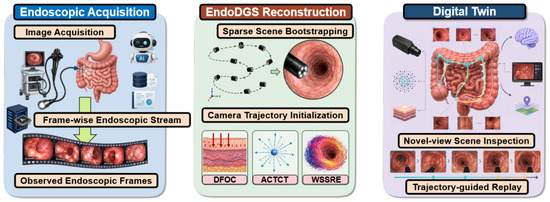
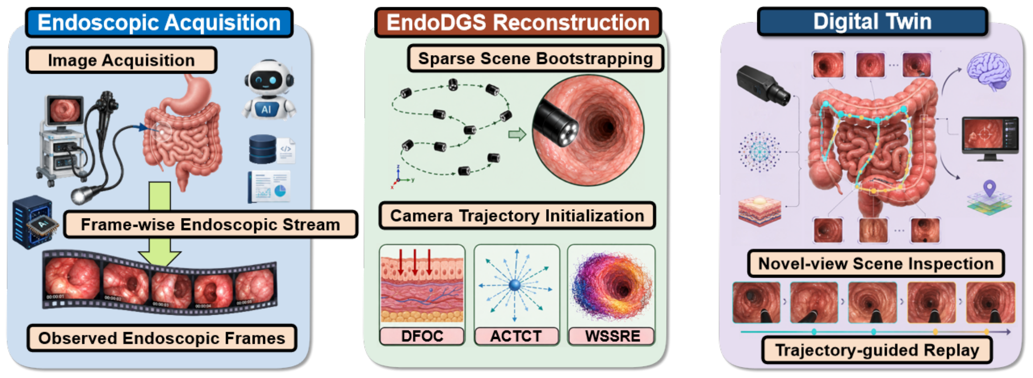
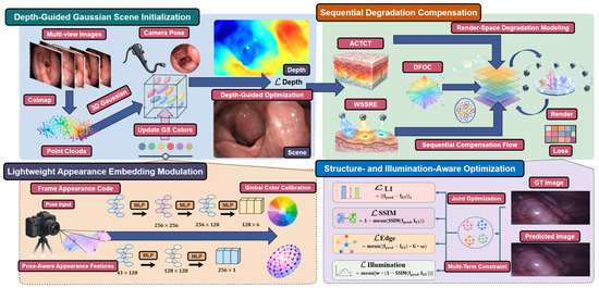
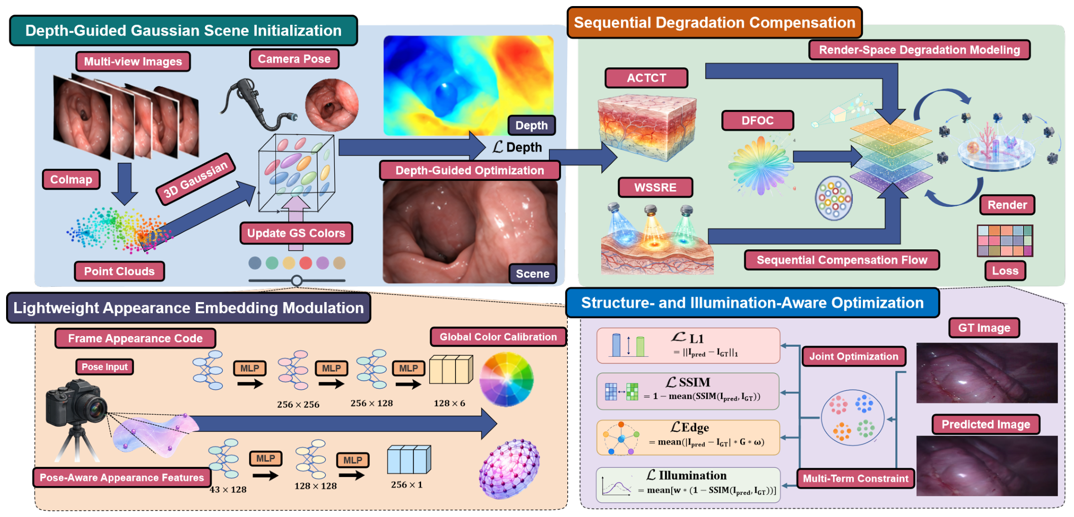
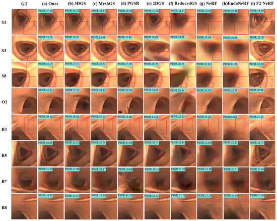
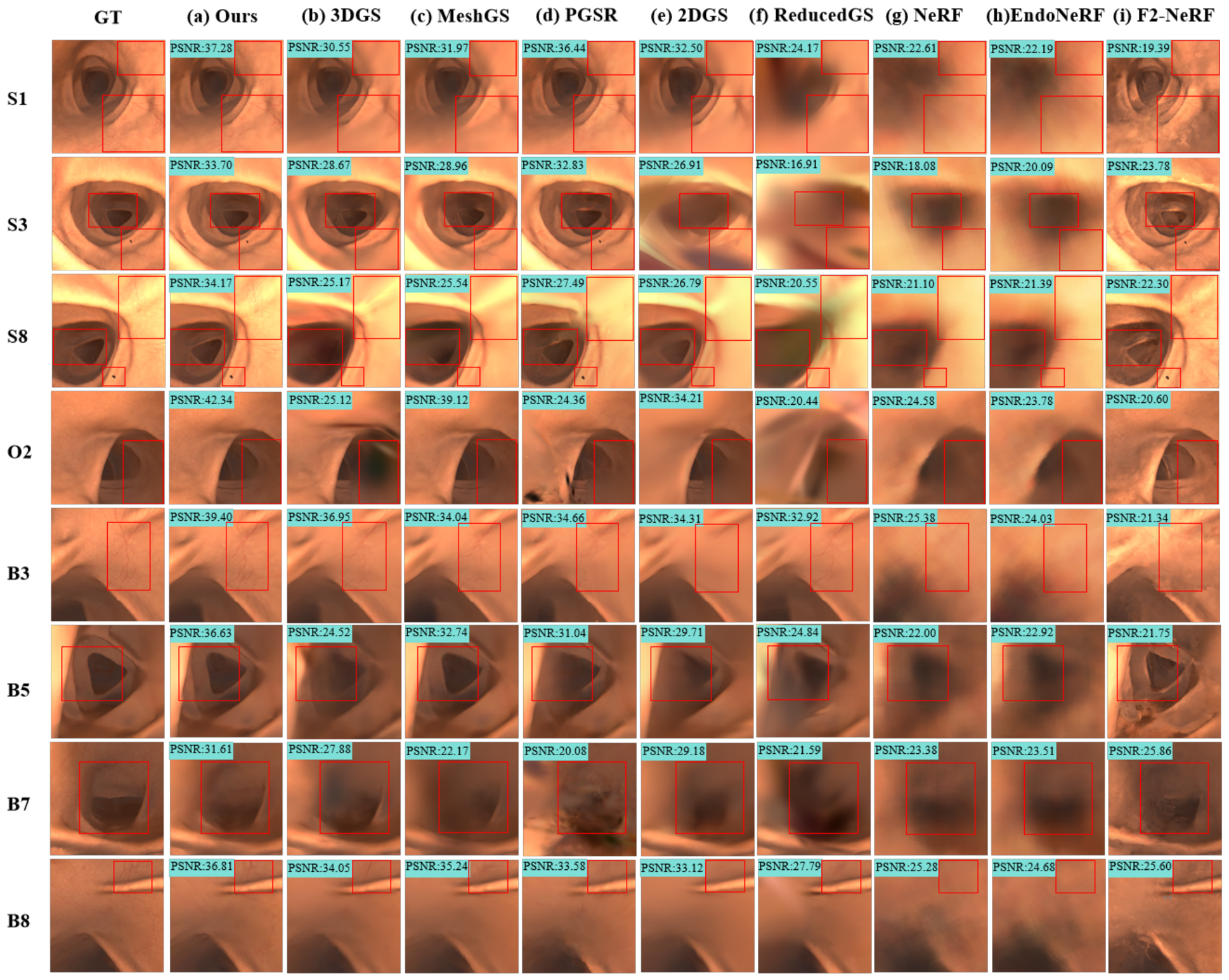
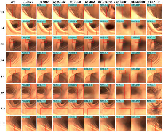
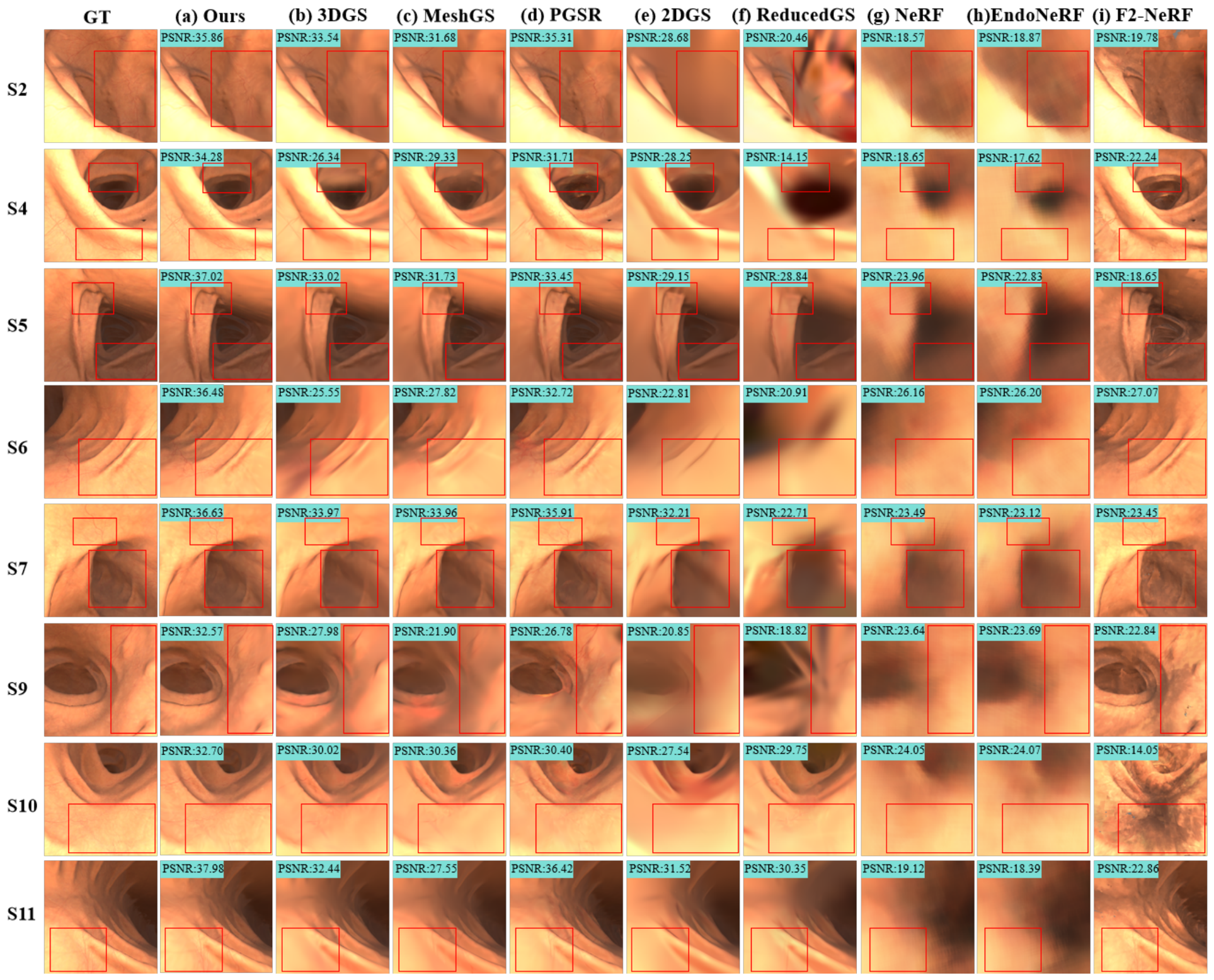
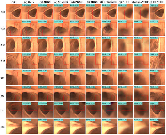
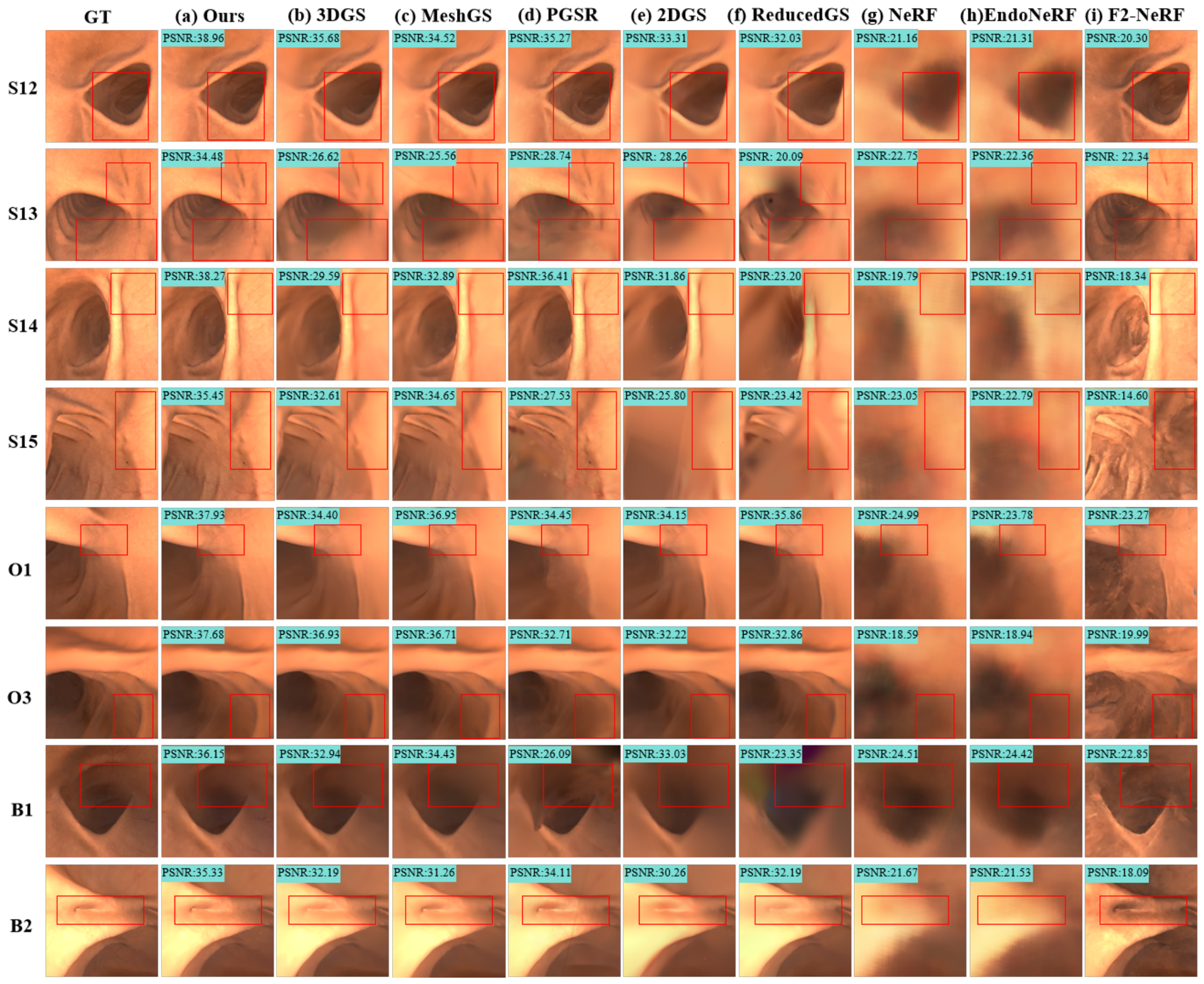
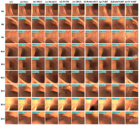
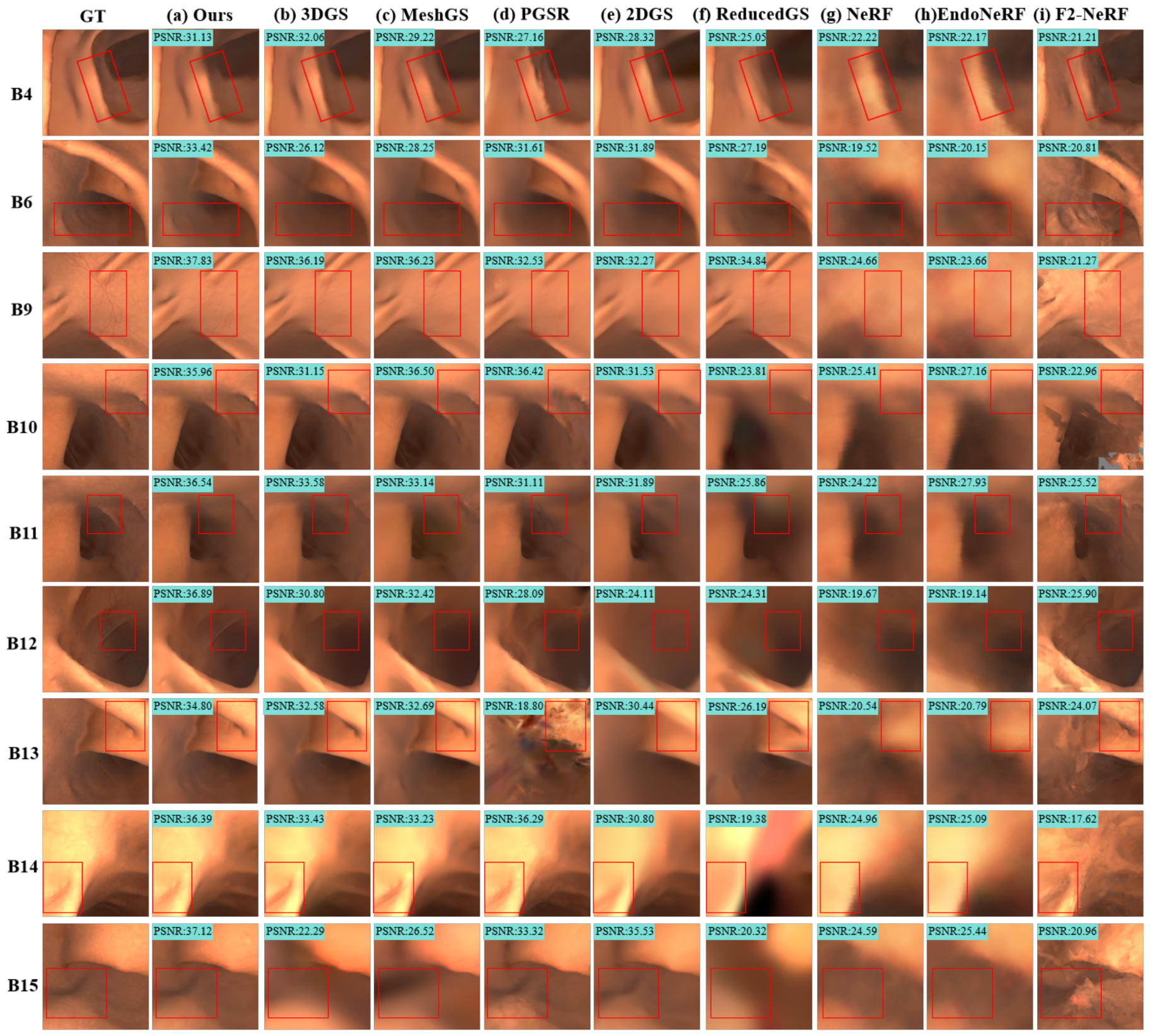
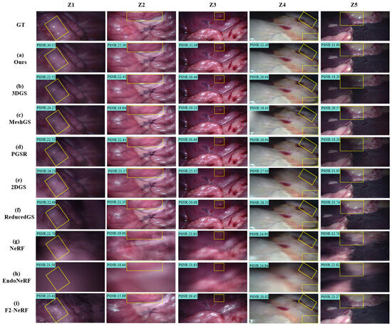
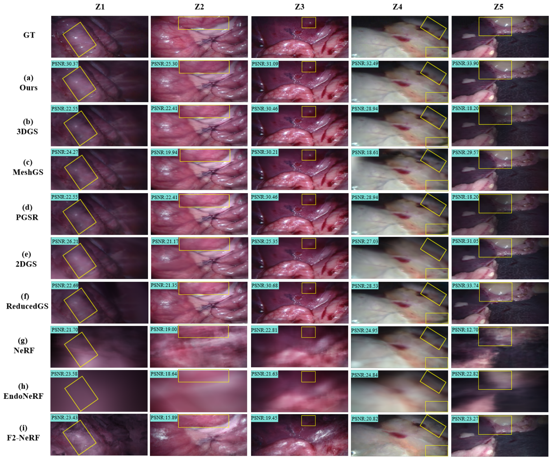
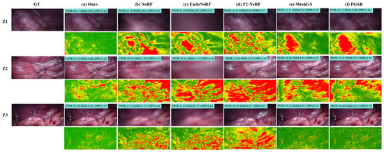
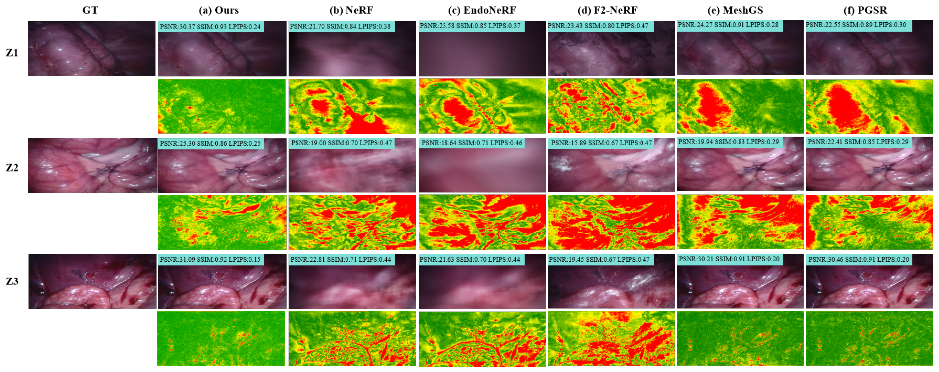



Disclaimer/Publisher’s Note: The statements, opinions and data contained in all publications are solely those of the individual author(s) and contributor(s) and not of MDPI and/or the editor(s). MDPI and/or the editor(s) disclaim responsibility for any injury to people or property resulting from any ideas, methods, instructions or products referred to in the content. |
© 2026 by the authors. Licensee MDPI, Basel, Switzerland. This article is an open access article distributed under the terms and conditions of the Creative Commons Attribution (CC BY) license.