Brillouin Optical Time Domain Reflectometry for Distributed Temperature Monitoring of Battery Energy Storage Systems

Abstract

The concept of Brillouin optical time domain reflectometry as a means of distributed temperature monitoring for battery systems is investigated and deemed feasible. The concept has been investigated regarding measurement speed, temperature accuracy, measurement range, and responsivity of the fiber material. The experiments show fast and accurate measurement results for surfaces with a uniformly distributed temperature, with an average absolute error of 0.51 K, a largest absolute error of 2.07 K, and a measurement time of approximately 60 s for a sampling point after 5 km. Additionally, hotspots only impacting 25% of the sensor fiber have been detected. Furthermore, the established concept provides a reliable and scalable solution for simultaneous temperature monitoring of spatially distributed sampling points without the need for individual cabling of every measurement sensor, like in commonly deployed electrical temperature detectors.

1. Introduction

Batteries are a key technology in the ongoing transformation towards an eco-friendly and sustainable society. Without battery energy storage systems (BESSs), the employment of solar and wind parks as main energy sources would not be feasible due to their volatile energy generation, which depends on environmental conditions such as weather and day-and-night cycle.

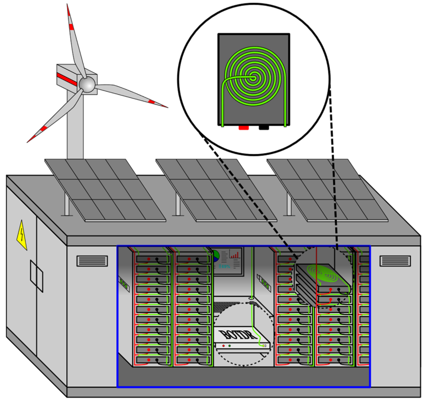
However, when malfunctioning due to damage or aging, batteries can generate great amounts of heat and hazardous gases, which by all means need to be avoided [1]. Therefore, monitoring and safety systems are employed. Especially BESSs, which can contain up to 3500 battery cells depending on the employed system, require fast and reliable monitoring, since one malfunctioning battery can set off a chain reaction which can propagate throughout the entire storage [2]. To guarantee reliable and fast monitoring, additional external monitoring systems, besides the battery management system (BMS) [3,4,5,6], which keeps track of current, voltage and other battery parameters, are employed to increase the safety by providing additional data and maintaining monitoring in the case of a BMS failure. A conceptual layout of such a BESS, with an additional external monitoring system, is depicted in Figure 1. These monitoring devices collect information about each battery cell, and the safety systems engage countermeasures if a behavior is registered which deviates from the intended safe behavior [7]. Typical parameters to determine the state-of-health of a battery are the surface temperature, the expansion of the battery casing, and the composition of the surrounding air [8]. Countermeasures are, for example, interruption of charging/discharging, and cooling of the battery cell [8]. However, these countermeasures are only effective as long as the battery has not entered the stage of a thermal runaway. At this point, heat generation is self-sustaining and cannot be stopped by external means [8].

Currently, several different external monitoring systems are employed or under consideration for employment in BESSs. Examples include resistance temperature detectors (RTDs) [9,10] and chained digital sensors (CDSs) [11], which are mounted to one or several points of the battery surface and monitor the surface temperature, and several optical fiber-based approaches, where a fiber is placed across the battery surface. These fiber-based approaches include Fiber Bragg Gratings (FBGs) [12,13] and Raman-based systems [14]. RTDs provide accurate and fast temperature measurements of individual batteries or even battery segments; however, each detector requires its own cable, making the installation and maintenance difficult for large BESSs. CDSs contain several sensors connected by a bus system. However, the approach is prone to electromagnetic interference due to the use of copper cables, making its deployment difficult, especially for safety-critical applications. Fiber-based approaches are more suitable for employment in BESSs. They are immune to electromagnetic fields, their polymer coating makes them insensitive towards acids, the fiber is small enough to be placed on the battery without interfering with the rack configuration, and a single fiber can interrogate several batteries, lowering the amount of employed cable.

However, the listed approaches have some drawbacks. FBGs are capped at, for example, 1000 per system depending on the interrogator, making them unsuitable for larger BESSs and, together with their small size, more suitable for temperature monitoring of small electrical components [15]. Raman-based systems have similar drawbacks, with Raman scattering being 30 dB weaker than Rayleigh scattering and 10 dB weaker than Brillouin scattering, offering a low signal-to-noise ratio (SNR), and therefore limiting its application in large BESSs due to its range [16].

The approach described in this work employs Brillouin optical time domain reflectometry (BOTDR). BOTDR can detect temperature and strain changes along the fiber, offers distributed sensing, and can employ a standard single mode fiber [17]. The main drawbacks are its high measurement time and low spatial resolution. However, by carefully choosing the measurement parameters and using an appropriate fiber placement, these disadvantages have been tackled and overcome.

Table 1. Performance comparison of different temperature measurement contenders (RTD = resistance temperature detector; CDS = chained digital sensor; FBG = Fiber Bragg Grating; Raman = Raman-based system; BOTDR = Brillouin optical time domain reflectometry).

	Cost	Accuracy	Measurement Time	Spatial Resolution	Capacity	Complexity	Robustness
RTD	medium	high	low	high	low	medium	high
CDS	low	medium	medium	high	medium	medium	low
FBG	high	high	low	high	medium	high	high
Raman	high	medium	high	medium	high	high	high
BOTDR	high	medium	high	medium	high	high	high

Green = high performance, Yellow = medium performance, red = low performance.

provides a comprehensive comparison of the different approaches and their respective performance in different categories. Cost refers to the acquisition cost, accuracy to the temperature accuracy, measurement time to the time between two consecutive measurements, spatial resolution to the dimensions of the measurement sensor, capacity to the number of sensors a system can support, complexity to the required installation and operation effort, and robustness to the ability of the system to operate under harsh environmental conditions, especially electromagnetic interference in the case of BESSs. Additionally, the performance parameters need to be put into perspective, regarding requirements and importance.

In our case, the system acts as an auxiliary safety system in an area where undetected malfunctions can lead to permanent damage of equipment and potential injuries of the personnel. Therefore, cost plays a subordinated role. Accuracy is an important parameter; however, the sub-kelvin accuracy of RTDs [9,10] and FBG-based systems [13] exceeds the system requirements. For the measurement time, similar circumstances apply. RTDs are capable of achieving measurement times in the millisecond regime; however, requirements rather range in the area of seconds. Spatial resolution is a rather complex topic. While a high spatial resolution is necessary to detect arising hotspots, it also increases the number of sensors required to cover the battery surface. The capacity is a key parameter for the system architecture. The system must be able to monitor all batteries employed in the BESS. For larger BESSs, the number of batteries can reach up to 3500. Complexity is similar to cost in safety-critical applications. Robustness is a main requirement. Since the system is safety-critical, it needs to provide reliable measurement values.

BOTDR has already been investigated for the structural health monitoring of infrastructure [18,19,20]. However, regarding the proposed application, additional requirements apply, which need to be put into consideration. First and foremost, fast and continuous measurements need to be guaranteed. While for structural health monitoring, measurement intervals of days, weeks, or even months are sufficient, battery monitoring requires measurement times of a few minutes or even less to mitigate an emerging thermal runaway [21]. The next aspect which needs to be investigated is the responsivity and thermal coupling of the optical fiber. Several sources investigated the achievable accuracy, range, and other parameters of BOTDR systems; however, in the used setups, the fiber has commonly been submerged in a liquid, e.g., water, or placed in an oven and been given plenty of time to reach the temperature of the medium [22,23,24,25,26].

The paper is organized as follows: In Section 2, the working principle of BOTDR, the setup, and the influence of parameters are described. In Section 3, the experimental setups are explained in detail. In Section 4, the results are presented and evaluated. In Section 5, the results are discussed and compared to other approaches. Finally, Section 6 concludes this study.

2. BOTDR Distributed Temperature Monitoring

2.1. BOTDR Principle for Temperature and Strain Sensing

BOTDR utilizes the physical phenomenon of Brillouin scattering. Thermal noise resulting from Brownian motion excites acoustic waves, which lead to a periodic change in the refractive index [27]. If the Bragg condition is fulfilled, the incoming light with wavelength ${\lambda }_{\mathrm{C}}$ experiences an inelastic scattering when interacting with the refractive index change:

$${\lambda }_{\mathrm{C}}=2n{\lambda }_{\mathrm{A}}\sin {\displaystyle \frac{\theta }{2}},$$

(1)

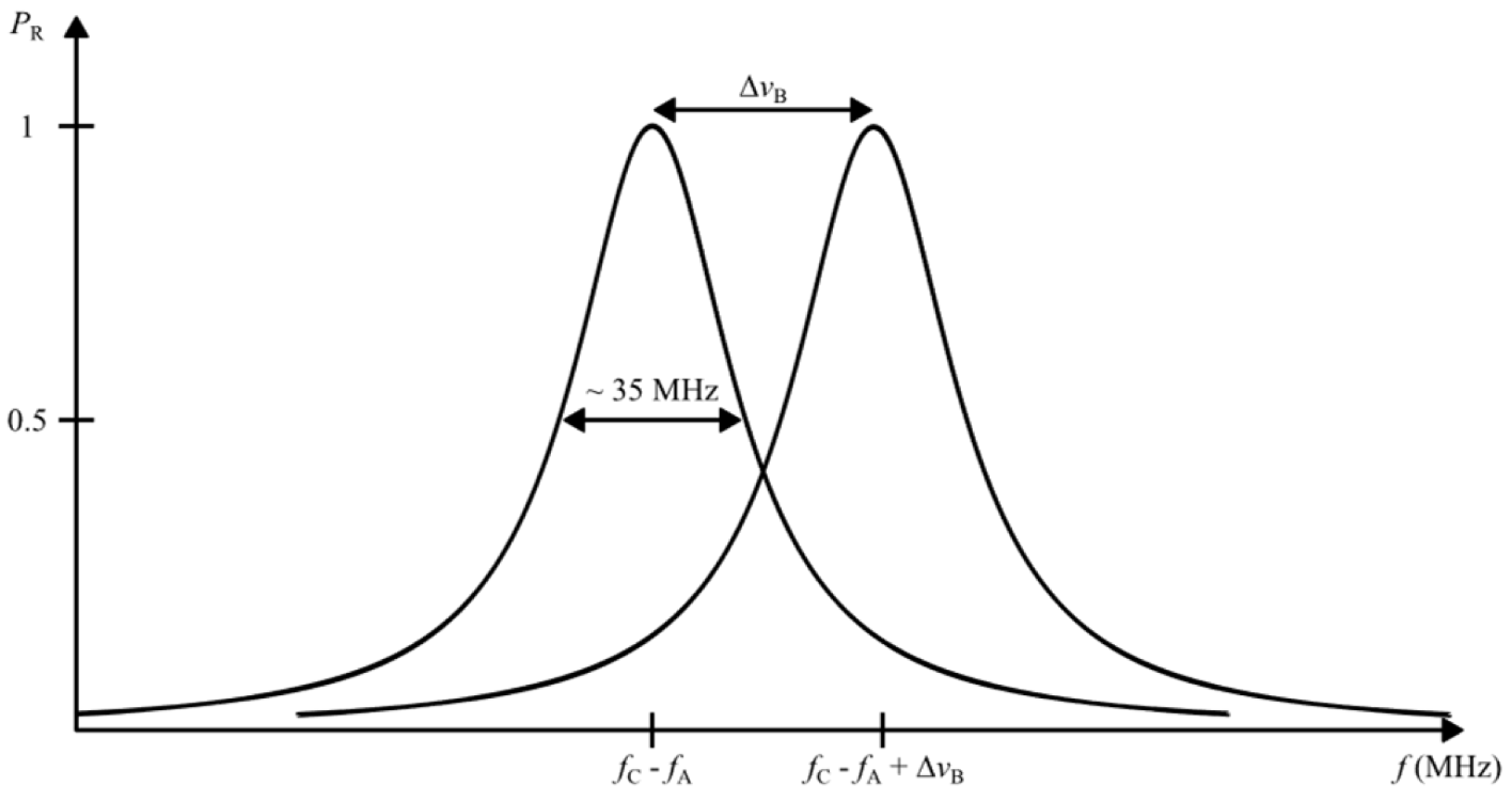
where n describes the refractive index of the medium, ${\lambda }_{\mathrm{A}}$ describes the wavelength of the acoustic wave and $\theta$ describes the angle between the incoming and the scattered wave [27]. While propagating in the opposite direction of the incoming wave, the backscattered light interacts with the incoming wave, transferring power from the incoming wave to the backscattered wave [27]. This process is called stimulated Brillouin scattering [27,28]. The backscattered light is downshifted from the carrier frequency, $f_{\mathrm{C}}$, by the acoustic frequency, $f_{\mathrm{A}}$. It exhibits a Lorentzian shape in the frequency spectrum, with a full-width at half-maximum (FWHM) of approximately 35 MHz [29]. However, for Brillouin scattering to occur, a minimal incoming pulse width of ~10 ns is required. This is due to the lifetime of the acoustic phonons, which is ~10 ns [27]. The frequency shift is commonly referred to as Brillouin frequency shift (BFS) and depends on the material, the concentration of the utilized dopants of the optical fiber, and the temperature and the applied strain in the environment of the fiber [30]. A temperature or strain difference $∆T$ or $∆\epsilon$, applied to the fiber, results in a linear shift of the BFS $∆v_{\mathrm{B}}$ and can be described using the appropriate formulas:

$$∆v_{\mathrm{B}}=c_{\mathrm{T}}· ∆T$$

(2)

and

$$∆v_{\mathrm{B}}=c_{\mathsf{\epsilon }}· ∆\epsilon ,$$

(3)

where $c_{\mathrm{T}}$ is the material-specific temperature coefficient and $c_{\mathsf{\epsilon }}$ is the material-specific strain coefficient. Using these formulas, a BFS change can be translated into the corresponding temperature or strain change. However, since both coefficients result in a BFS change, it is not possible to attribute the BFS change to the corresponding parameter. Therefore, it is required that only one parameter changes between two measurements. A shift due to a change in strain or temperature is shown in Figure 2.

2.2. System Setup

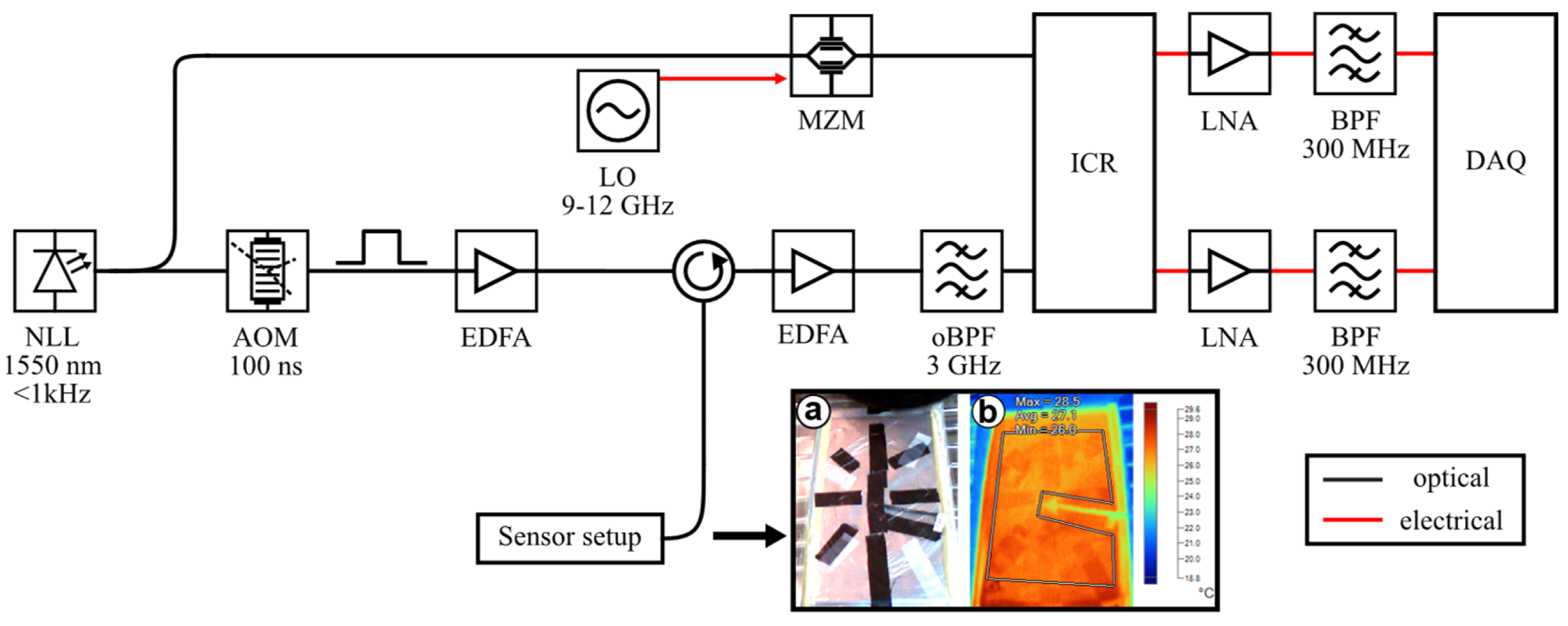
The system setup with a connected fiber sensor applied to a battery is depicted in Figure 3. As the light source, a narrow linewidth laser (NLL) has been chosen, which emits a continuous wave (CW) with a vacuum wavelength of 1550.12 nm and a linewidth < 1 kHz. This laser surpasses the requirements for BOTDR and is employed since parts of the setup are used for coherent optical time domain reflectometry, which has higher requirements regarding laser linewidth. Laser linewidths below 1 MHz barely provide additional benefits when it comes to BOTDR [31]. A polarization-maintaining coupler splits the optical power into two paths. The first path serves as a local oscillator (LO), while the second path feeds the signal into an acousto-optic modulator (AOM). The AOM is used to modulate a rectangular-shaped probing signal onto the CW signal. For the experiments, pulses with a duration of 100 ns are generated. Translating the duration into a length equals a spatial resolution of approximately 10 m. After the pulses are generated, they are amplified by an Erbium-doped fiber amplifier (EDFA). The pulses are then fed into the optical circulator and the sensor setup. In order to obtain the required Brillouin scattering, several steps are necessary. At first, the backscattering is amplified by again using an EDFA. Afterwards, an optical band-pass filter (oBPF) is applied, which suppresses the Rayleigh scattering components, which need to be suppressed due to their relatively high power compared to the power of the Brillouin backscattering. Afterwards, the signal reaches an integrated coherent receiver (ICR). It is necessary to separate the Brillouin scattering in space and frequency. In order to sample the Brillouin frequency spectrum, the backscattered light is superimposed with the light from the LO path. The electro-optic modulator (EOM) modulates a subcarrier based on a sinusoidal radio frequency signal on the LO, which applies a subcarrier modulation. It is possible to vary the subcarrier frequency between 9 GHz and 12 GHz, depending on the Brillouin scattering of the sensor fiber. The superimposed signal is transferred into the baseband and, afterwards, amplified by a low-noise amplifier (LNA) before being filtered again by an electrical band-pass filter (BPF). In the end, the signal is evaluated by a data acquisition system (DAQ). The DAQ is formed by an analog-to-digital converter (ADC) and a field-programmable gate array. The system exhibits a sampling rate of approximately 250 MSa/s, resulting in a spatial sampling step of ~0.4 m.

2.3. Signal Processing

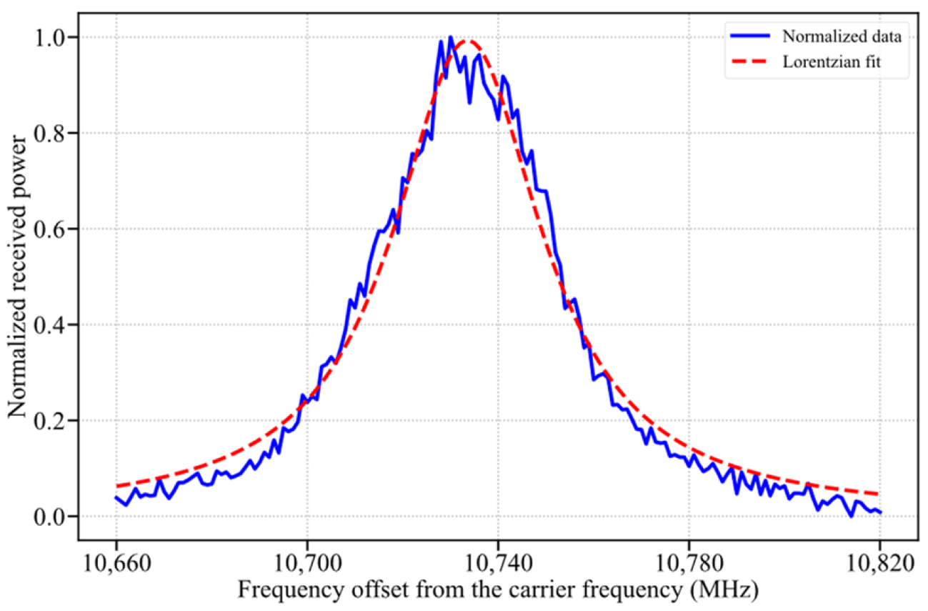
In order to increase the measurement accuracy of the system, the received signal is further processed. Firstly, the background noise is reduced by subtracting the noise which occurs when no signal or backscattering is present, from the received signal. Afterwards, the signal is normalized for easier processing. In the last step, a curve fitting is applied. The curve fitting utilizes the Lorentzian shape of the Brillouin backscattering over the spectrum. It acts as a low-pass filter, which reduces the impact of noise and increases the accuracy, since the fitting is not restricted to the distinct frequency steps. The impact of a curve fitting applied to a received signal over the spectrum is displayed in Figure 4.

2.4. Placement of the Fiber

To successfully measure an object’s temperature, it is important that the whole pulse is confined to the fiber attached to the object. The reason for that is that the backscattered power accumulates, meaning that the resulting received power trace over the frequency contains all temperatures present in the fiber section interrogated by the pulse. The impact of each temperature is proportional to the amount of fiber it occupies. Hence, increasing the pulse width increases the SNR, but also the amount of fiber impacting the measurement. Therefore, in order to achieve accurate temperature values, the pulse width and the spatial sampling step need to be considered. The pulse width of 100 ns, which translates to a ~10 m spatial resolution, means that at least 10 m of fiber on the object is required. Additionally, 1 m of fiber has been added so that, with a spatial sampling step of ~0.4 m, at least one sampling point exists where the whole pulse is confined to the fiber. In order to attach 11 m of fiber to the object, the fiber has been spooled in a spiral shape. This reduces its dimensions to approximately 15 × 15 cm, without applying additional strain to the fiber due to bending. When deployed in BESSs, the fiber should be mounted to the battery surface using an adhesive material, which exhibits a good thermal coupling and a high elasticity. Configurations where the fiber is wrapped around the object have been discarded, since the bending radius of the fiber leads to large parts of the fiber not being in contact with the object. The infrared imaging, visible in Figure 3b, suggests a uniform temperature distribution along the surface under normal conditions, enabling the proposed configuration for accurate temperature measuring. However, in the case of an emerging thermal runaway, smaller hotspots often arise at the surface area in close proximity to the malfunctioning cell. As a result, there is no longer a uniform surface temperature. This aspect requires additional consideration when it comes to omitting thermal runaways.

2.5. Influence of Choice of System Parameters

The frequency range, limited by the start frequency $f_{\mathrm{s}}$ and end frequency $f_{\mathrm{e}}$, determines the temperature and strain range the system can monitor. The frequency range is proportional to the measurement time. The step size $s$ defines the distance between adjacent measurement frequencies. Increasing the step size lowers the number of measured frequencies and therefore reduces the measurement time. However, it also lowers the measurement accuracy of the system. The number of averages $n_{\mathrm{a}}$ describes the amount of accumulated backscatter traces per measurement frequency. Increasing the number of averages increases the SNR while also increasing the measurement time. The number of measurements, $n_{\mathrm{m}}$, per measurement run can be calculated using the following.

$$n_{\mathrm{m}}={\displaystyle \frac{\left({|f}_{\mathrm{e}}-f_{\mathrm{s}}|\right)}{s}}·n_{\mathrm{a}} .$$

(4)

For the experiments, the parameters $f_{\mathrm{s}}= f_{\mathrm{c}}-\mathrm{10,660} \mathrm{M}\mathrm{H}\mathrm{z}$, $f_{\mathrm{e}}= f_{\mathrm{c}}-\mathrm{10,820} \mathrm{M}\mathrm{H}\mathrm{z}$, and $s=1 \mathrm{M}\mathrm{H}\mathrm{z}$ have been chosen, with $n_{\mathrm{a}}$ varying between 5000 and 6000, depending on the time constraints of the experiment.

3. Measurement Configuration

3.1. Temperature Sensing Using a Single Heating Plate

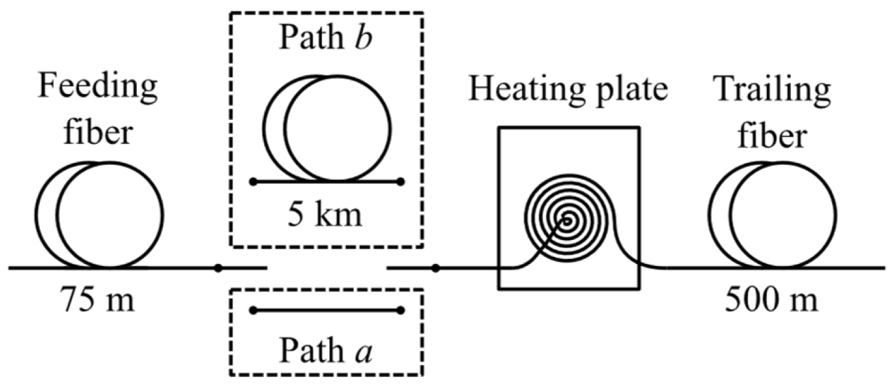
The setup for the first experiment is depicted in Figure 5. The pulse is emitted into the fiber. Firstly, it traverses 75 m of feeding fiber. This fiber is used as a connector between the interrogator and measurement setup. Afterwards, it either directly enters path (a), the fiber sensor placed on the heating plate, or enters path (b), a 5 km fiber spool, which is used to simulate the attenuation when used in a monitoring setup, before entering the fiber sensor. Finally, it reaches the 500 m of trailing fiber, which is connected so that no reflections from the open angled connector interfere with the backscattering from the sensor. For better mounting of the sensor, a heat-conducting film has been placed on top of the heating plate before placing the sensor.

Two measurement runs are conducted for each path. In the first run, the temperature is increased in steps of 10 K, starting at 30 °C, until reaching 70 °C, with a settling time of roughly 6 min per step. In the second run, the temperature is increased rapidly from roughly 30 °C to 70 °C. An RTD with a temperature resolution of 1 K and a sampling frequency of 1 Hz is also attached to the heating plate to provide a reference value. The first run is conducted to determine the temperature coefficient. The results from the BOTDR interrogator are compared to the reference values, and the temperature coefficient yielding the lowest deviation is chosen. The second run is conducted to determine the temperature accuracy. The results from the BOTDR interrogator are divided by the previously determined temperature coefficient and compared to the reference values.

3.2. Hotspot Detection Using a Single Heating Plate

In the next experiment, the previously employed setup is used again. However, only the upper left quarter of the spiral is placed on the heating plate. Afterwards, the heating plate is heated up to 70 °C. This experiment simulates an arising hotspot, only impacting part of the sensor.

3.3. Distributed Sensing Setup Using Temperature Chambers

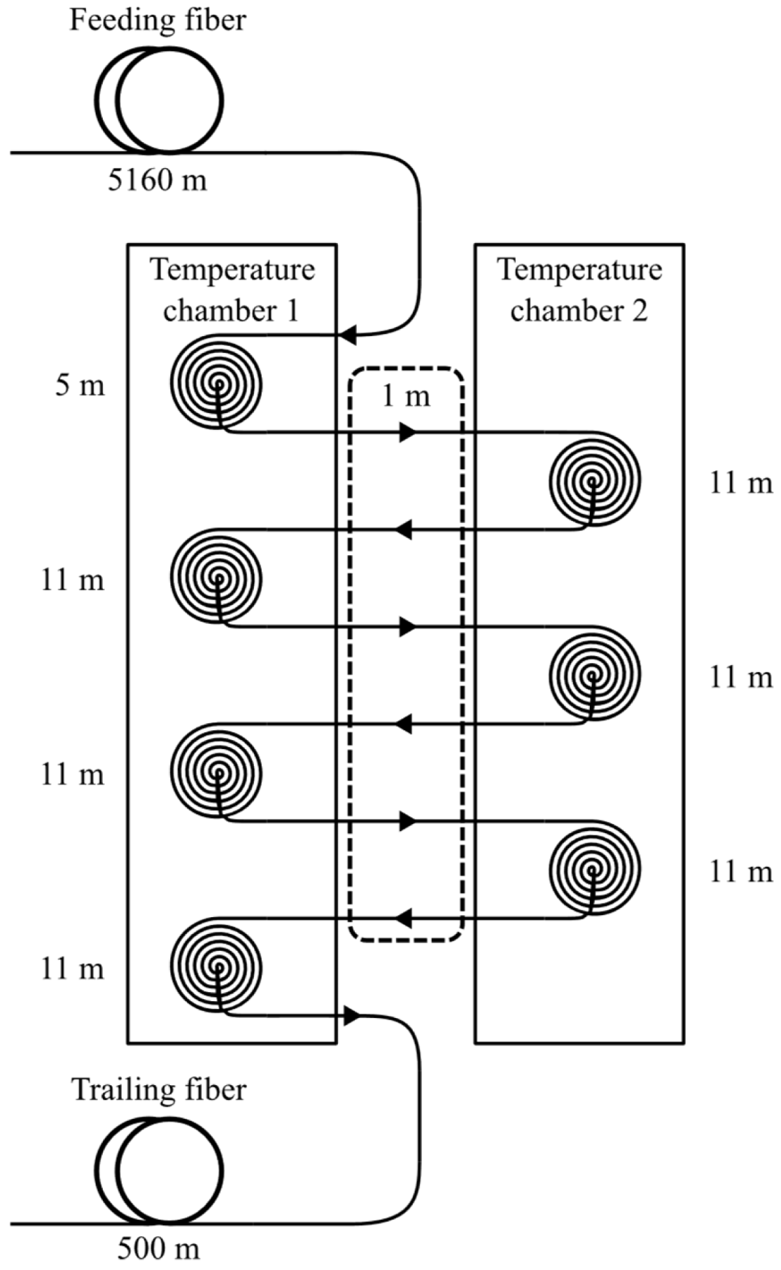
The setup for the third experiment is depicted in Figure 6. The pulse is entering the 5.16 km feeding fiber, connecting the BOTDR interrogator with the sensor. The sensor consists of a setup with two independent temperature chambers (TCs). The fiber is arranged in 7 distinct spools, with the first one being 5 m in length, while the rest are 11 m in length. The spools are placed alternatingly in the two TCs, connected by 1 m of optical fiber, beginning with TC 1. The last spool is connected to a trailing fiber with an open-angled physical connector, which prevents reflections from the connector interfering with the measurement results.

The temperatures in the TCs are set to 10 °C and 70 °C, respectively. During the measurement run, the temperatures are increased and decreased, respectively, in steps of 10 K, until they have reached each other’s starting temperature. The temperature in the TCs is either higher or lower than the ambient temperature and the temperature in the other TC. Since the received power over the frequency spectrum accumulates over the whole extension of the pulse, parts of the pulse which are located outside the TC would increase or decrease the measured BFS, depending on the ambient temperature. Hence, the maximum or, respectively, minimum temperature, which equals the temperature of the corresponding TC, is only achieved at sampling points where the whole pulse is confined to the fiber inside the TC. Due to the chosen parameters, as discussed in Section 2.4, at least one such sampling point exists per spool.

4. Results

4.1. Determination of the Temperature Coefficient

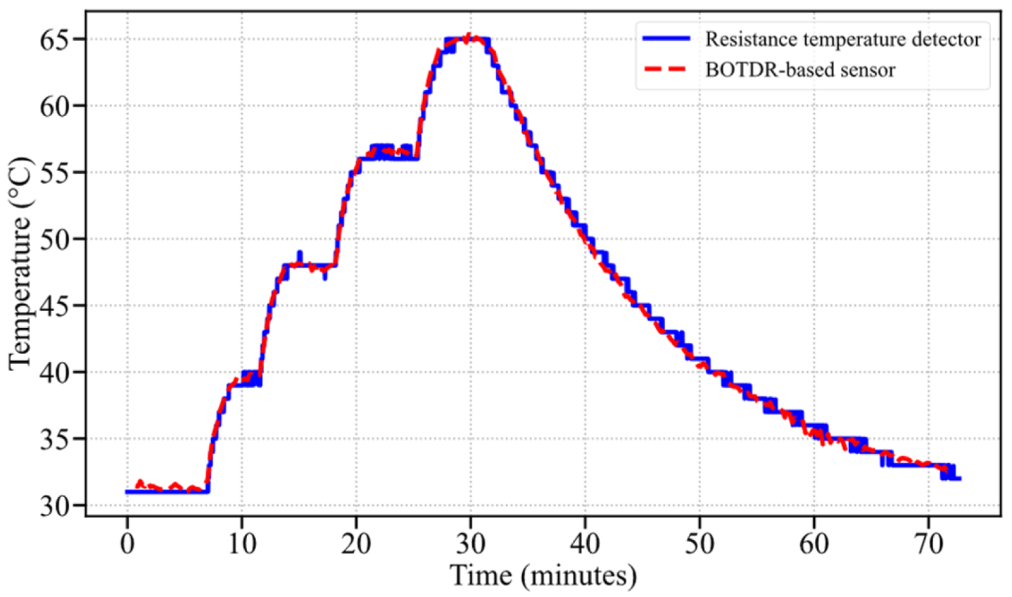
Overall, 329 individual measurements have been conducted over a time frame of roughly 72 min and a temperature range of approximately 35 K, with the setup illustrated in Figure 5a. The temperature coefficient obtained from the experiment is $c_{\mathrm{T}}~1.15 \mathrm{M}\mathrm{H}\mathrm{z}/\mathrm{K}$, which is in close proximity to the value for a standard single-mode fiber provided in the established literature [18]. Inserting this value into Equation (2), and rearranging it according to $∆T$, yields the corresponding temperature change based on the BFS change. In Figure 7, the temperature as a function of time is depicted for the BOTDR and the RTD sensor. Here, the temperature obtained with the BOTDR approach is compared to the temperature of the RTD sensor. It can be seen that both sensors follow the adjusted temperature parameters.

4.2. Comparison to Baseline Temperature Measurements

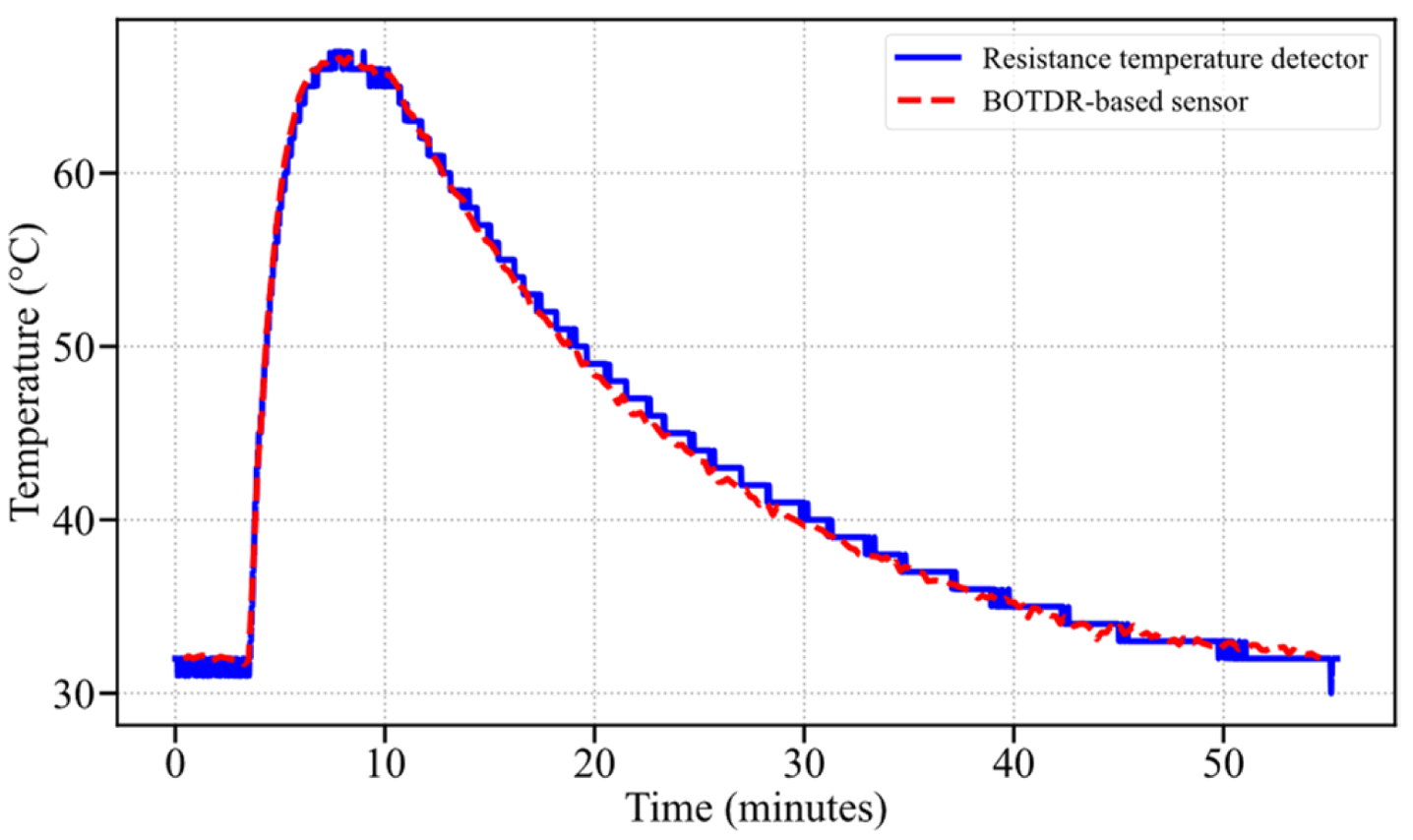
In the second measurement run, the accuracy and responsivity of the system were evaluated. For this experiment, a measurement range of 30 °C to 70 °C was chosen. In order to simulate a fast temperature change, the temperature of the heating plate was set to 70 °C after it settled at around 30 °C. Figure 8 shows the converted temperature based on the BFS variation and the RTD sensor as a function of time. Comparing the two traces, an average absolute error of less than 0.52 K and a maximum error of less than 1.45 K were obtained. In addition, the steepest 60 s interval, ranging from 3:31 min to 4:31 min, was determined, leading to a maximum temperature gradient of 22 K/min. These results show that a surface-mounted, spiral-shaped fiber exhibits excellent thermal coupling with the object it is exposed to. In order to put these results into perspective, the temperature increase has been compared to the temperature changes of a battery. An overcharged pouch cell exhibits, after venting at 51 °C, a temperature gradient of approximately 13 K/min before entering the state of a thermal runaway after an additional 3.6 min [21]. Since the temperature gradient of the experiments conducted with the fiber-based sensor setup of Figure 5a is approximately 1.69 times higher than the temperature gradient of an overcharged pouch cell prior to entering a thermal runaway, the responsivity of the fiber-based sensor setup is deemed sufficient.

4.3. Hotspot Detection

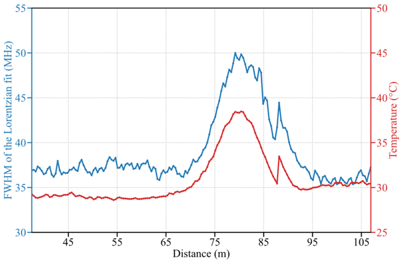
The experiment introduces a temperature change along an accumulated fiber length of roughly 2.75 m, which is below the required 10 m imposed by the chosen pulse width. An accurate temperature measurement is therefore not possible. However, the hotspot is still impacting the measurement and raising the measured temperature above the value of the ambient air temperature. In order to distinguish between a small, uniformly distributed, and a high, local temperature increase, the width of the Lorentzian shape can be utilized. While a constant temperature along the whole measurement section leads to an accumulation of Lorentzian shapes, which all exhibit the same frequency offset, the presence of a hotspot leads to an accumulation of Lorentzian shapes with different frequency shifts. This results in a higher FWHM of the Lorentzian shape, which is depicted in Figure 9. This allows the approach to identify hotspots far below its nominal resolution, but at the expense of not being able to determine the exact temperature of the hotspot. The FWHM acts as an integrated control parameter, providing information about the temperature composition.

4.4. Distributed Sensing

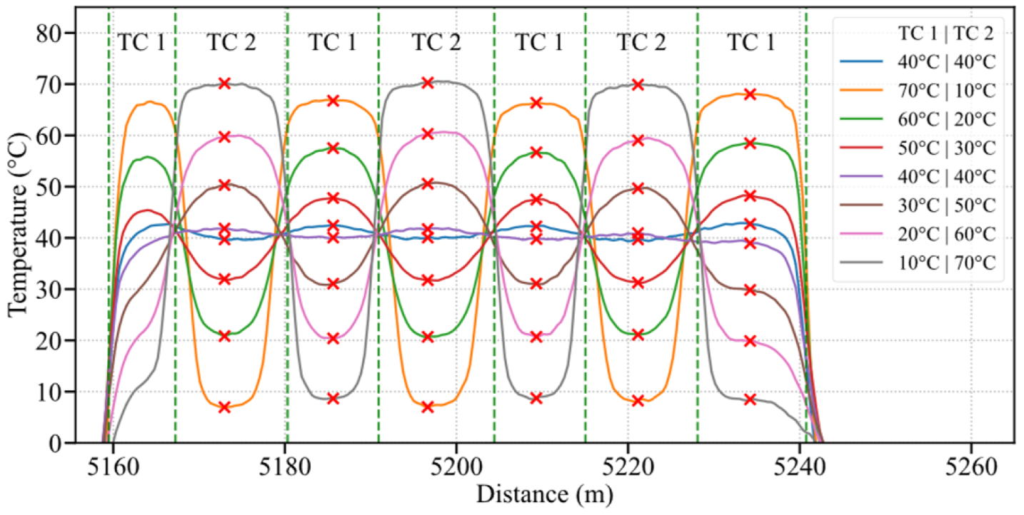
The experiment based on the setup depicted in Figure 6 yielded accurate results regarding the allocation of sampling points to specific fiber sensors. In Figure 10, several traces in different temperature configurations are depicted. For each spool, the BFS converges towards a certain value. This value is reached when the whole pulse is confined to the fiber inside the TC. Due to the chosen configuration, at least one such measurement point exists per spool. For the sampling points these measurement points have been chosen and marked with a red cross in the figure. It is also visible that spools inside the same TC reach similar temperature values, hinting the possibility of simultaneous monitoring of several measurement points.

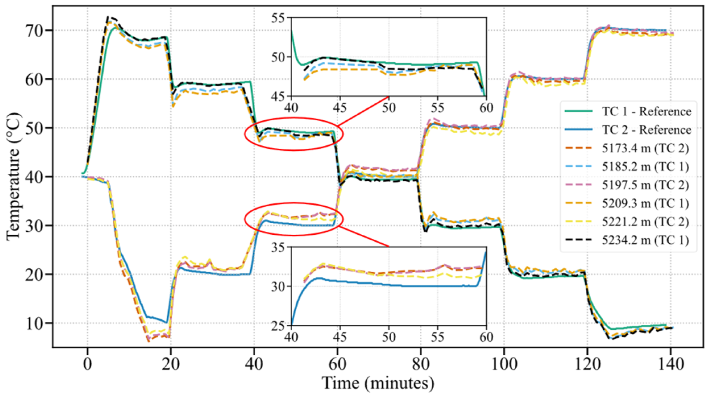
In Figure 11, the temperature traces of all determined sampling points are depicted and compared to the reference value provided by the TC. It can be seen that all pre-determined sampling points are capable of displaying temperature values in proximity to the reference temperature. Higher deviations and other errors can be attributed to the temperature regulation of the TCs, which operates via airflow and tends to have a higher cooling/heating impact on the loosely placed spool than on the rather compact temperature detector implemented in the TCs. For all sampling points inside the same TC, a shared temperature coefficient was used. The circumstance that all temperature coefficients were similar, and a shared temperature coefficient yielded accurate results, indicates similar material properties along the fiber, which simplifies the installation, since parameters like the temperature coefficient can be assumed to be constant over the whole fiber. Also, the accuracy remained constant over the course of the experiment, which means that the sampling points did not vary throughout the experiment. This shows that the approach is capable of monitoring multiple objects simultaneously over a longer time with a good temperature accuracy.

4.5. Measurement Accuracy

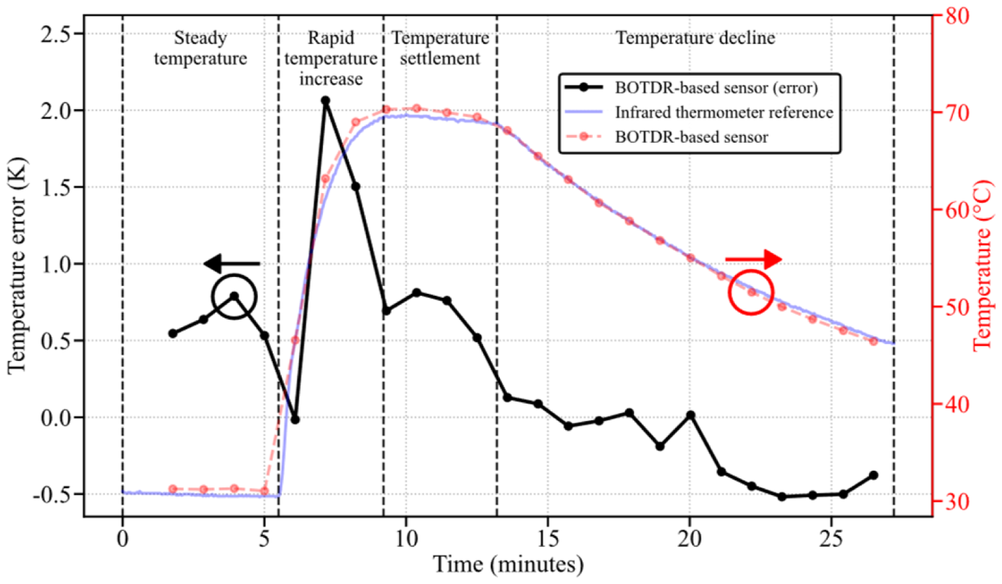
The results obtained by employing the setup depicted in Figure 5b prove the feasibility of the BOTDR approach for distributed temperature monitoring. The deviation of the BOTDR trace from the reference trace, provided by an infrared thermometer with a temperature resolution of 0.1 K and a sampling frequency of 1 Hz, is presented in Figure 12. The comparison of the two traces shows an average absolute error of less than 0.51 K, and a maximum error of less than 2.07 K. The sensor was placed after 5 km of feeding fiber. Since the accuracy of the system can be attributed mainly to the SNR, which is steadily declining along the fiber, it is reasonable to assume that the sensor farthest away exhibits the lowest SNR of the monitored sensors and, hence, the lowest accuracy. The acquisition of all frequencies takes approximately 60 s. Considering the transient nature of the temperature in this experiment, allocating the temperature value to the center of the time frame seems appropriate, and is reaffirmed by the results. The results show that the chosen approach is capable of accurately measuring temperature traces of surfaces exhibiting a uniformly distributed surface temperature, even if the temperature changes throughout the measurement run.

5. Discussion

In our work, we have shown the potential of BOTDR for temperature monitoring. While FBG-based approaches require multiple point-sensors per battery, depending on the surface area, to cover all possible locations of arising hotspots, the spiral shape can cover larger areas of the surface and still detect anomalies by evaluating BFS and FWHM. Additionally, our approach does not require a special fiber. RTDs suffer similar problems regarding surface coverage. While the small measurement area enables the accurate temperature determination of hotspots, it also carries the risk of missing them if the hotspot arises at a location not covered by a sensor. An additional drawback is the cable management, since each sensor requires a dedicated cable. One of the major drawbacks of our approach is the loss of temperature determination capabilities in the case of a non-uniform temperature distribution as a result of an arising hotspot. However, this does not impair its functionality. While the batteries work properly, the temperature is distributed uniformly, enabling accurate temperature monitoring and allowing the BMS to make decisions based on this information. In the case of unintended behavior, the temperature distribution becomes non-uniform due to, for example, an arising hotspot, prohibiting accurate temperature determination. However, the temperature of the hotspot is not the important aspect, but rather the timely detection of such is, so that appropriate countermeasures can be taken. This condition is still fulfilled by our approach.

6. Conclusions

Our studies show the feasibility of Brillouin optical time domain reflectometry in the context of individual battery temperature monitoring in battery energy storage systems. Battery cell, optical fiber, and measurement approaches were investigated and adjusted so the parameters were in accordance with the requirements of battery energy storage systems. The temperature profile of the battery surface was investigated, and the approximately uniform temperature distribution during intended behavior enables the arbitrary positioning of the temperature sensor. This justifies the placement of larger amounts of fiber across the surface without losing temperature information or accuracy. Hence, the deployment of an optical fiber in a spiral shape is eligible. This circumstance resolves the most severe drawback of Brillouin optical time domain reflectometry in fields containing small monitoring objects: its minimum spatial resolution of 1 m. While a uniform temperature distribution is required for accurate temperature monitoring, the hotspot experiment shows that emerging temperature anomalies only influencing 25% of the fiber sensor can be identified by evaluating the width of the Lorentzian shape. This is a major advantage compared to point sensors, since the fiber covers a larger area, making the occurrence of hotspots in monitored areas more likely. The experiments regarding fast temperature rise have shown that the optical fiber is capable of adapting to temperature changes in a fast manner, even in a surface-mounted configuration. Also, the Brillouin optical time domain reflectometry approach has displayed accurate results under transient temperature conditions. Lastly, the experiments in the temperature chambers have shown that simultaneous monitoring of multiple battery cells is possible. Based on these results, the deployment of Brillouin optical time domain reflectometry for individual battery cell temperature monitoring in battery energy storage systems is deemed feasible.

References

1. Zalosh, R.; Gandhi, P.; Barowy, A. Lithium-ion energy storage battery explosion incidents. J. Loss Prev. Process Ind. 2021, 72, 104560. [Google Scholar] [CrossRef]
2. Kruse, L.E.; Schill, J.; Landsiedel, O.; Pachnicke, S. Optical Monitoring of Second-Life Batteries Enhanced by Machine Learning. In Proceedings of the 2022 IEEE 13th International Symposium on Power Electronics for Distributed Generation Systems (PEDG), Kiel, Germany, 26–29 June 2022; pp. 1–5. [Google Scholar] [CrossRef]
3. Kyeremeh, K.A.; Lavin, S.E.; Fischer, G.M.; Ionel, D.M.; Patrick, A. Utility-Scale Battery Energy Storage Systems—Field Pilot Unit Experience, Analysis, and Review of Technological Advancements. IEEE Access 2026, 14, 74274–74288. [Google Scholar] [CrossRef]
4. Thirupathamma, S.; Veerapaneni, S.J.; Chillabanda, V.; Pothireddy, V.V.R.; Kuna, S.; Devarapalli, S.B.; Deshpande, A.P.; Samanta, S. State-of-Health Prediction of Lithium-Ion Batteries Using Physics-Informed Inverted Attention Transformer. In Proceedings of the 2026 International Conference on Intelligent Processing, Hardware, Electronics, and Radio Systems (CIPHER); IEEE: New York, NY, USA, 2026; pp. 1–6. [Google Scholar] [CrossRef]
5. Zhou, Z.; Lyu, T.K.; Nguyen, P.; Kim, S.; Park, J.W. State-of-Health Estimation in NCA Lithium-Ion Batteries Using Incremental Capacity Analysis and Gaussian Process Regression While Considering Capacity Recovery. In Proceedings of the 2026 IEEE Applied Power Electronics Conference and Exposition (APEC); IEEE: New York, NY, USA, 2026; pp. 3007–3012. [Google Scholar] [CrossRef]
6. Chen, Q.; Duan, K.; Miao, W.; Sun, X. Non-invasive Lithium Battery Diagnosis by Magnetic Field Sensing and Machine Learning Assisted Recognition. In Proceedings of the 2026 11th Asia Conference on Power and Electrical Engineering (ACPEE); IEEE: New York, NY, USA, 2026; pp. 1315–1319. [Google Scholar] [CrossRef]
7. Ding, Z.; Shi, Q.; Yao, H.; Zhang, Z.; Liu, Z. Study on Fire Suppression of Lithium-Ion Battery Module by Perfluorohexanone. In Proceedings of the 2026 5th International Conference on Smart Grid and Green Energy (ICSGGE); IEEE: New York, NY, USA, 2026; pp. 902–905. [Google Scholar] [CrossRef]
8. IEEE Std 2686-2024; IEEE Recommended Practice for Battery Management Systems in Stationary Energy Storage Applications. IEEE: New York, NY, USA, 2025; pp. 1–89. [CrossRef]
9. Cai, Q.; Chen, Y.-C.; Tsai, C.; DeNatale, J.F. Development of a platinum resistance thermometer on the silicon substrate for phase change studies. J. Micromech. Microeng. 2012, 22, 085012. [Google Scholar] [CrossRef]
10. Koshkouei, M.J.; Saniee, N.F.; Barai, A. Accurate Surface Temperature Monitoring of Lithium-Ion Batteries. In Proceedings of the 2024 IEEE Transportation Electrification Conference and Expo (ITEC), Chicago, IL, USA, 19–21 June 2024; pp. 1–5. [Google Scholar] [CrossRef]
11. Wang, J. Design Intelligent Temperature Monitoring System Based on DSP. In Proceedings of the 2012 4th International Conference on Intelligent Human-Machine Systems and Cybernetics; IEEE: New York, NY, USA, 2012; pp. 234–237. [Google Scholar] [CrossRef]
12. Ding, Z.; Hou, Y.; Gao, H.; Zhong, J.; Yu, D.; Chen, Y.; Zhan, C.; Zhao, C. Chirped-FBG-assisted weak-FBG demodulation method and its application in quasi-distributed temperature sensing and battery monitoring. IEEE Internet Things J. 2026, 1. [Google Scholar] [CrossRef]
13. Huang, F.; Yang, H.; Liu, B.; Liu, J.; Hu, Y.; Fu, Y.; Xiao, W.; He, X.-D.; Wu, Q. Real-Time Monitoring of Temperature Field Distribution of Three-Element LiB Lithium Battery Using FBG Arrays. IEEE Sens. J. 2023, 23, 30473–30480. [Google Scholar] [CrossRef]
14. Li, J.; Zhang, Q.; Xu, Y.; Zhang, M.; Zhang, J.; Qiao, L.; Promi, M.M.; Wang, T. High-accuracy distributed temperature measurement using difference sensitive-temperature compensation for Raman-based optical fiber sensing. Opt. Express 2019, 27, 36183–36196. [Google Scholar] [CrossRef] [PubMed]
15. Isa, R.; Iqbal, N.; Abido, M.; Mirza, J.; Qureshi, K.K. Multipoint Thermal Sensing System for Power Semiconductor Devices Utilizing Fiber Bragg Gratings. Appl. Sci. 2024, 14, 11328. [Google Scholar] [CrossRef]
16. Horiguchi, T.; Shimizu, K.; Kurashima, T.; Tateda, M.; Koyamada, K. Development of a distributed sensing technique using Brillouin scattering. J. Light. Technol. 1995, 13, 1296–1302. [Google Scholar] [CrossRef]
17. Maraval, D.; Gabet, R.; Jaouen, Y.; Lamour, V. Dynamic Optical Fiber Sensing with Brillouin Optical Time Domain Reflectometry: Application to Pipeline Vibration Monitoring. J. Light. Technol. 2017, 35, 3296–3302. [Google Scholar] [CrossRef]
18. Bai, Q.; Wang, Q.; Wang, D.; Wang, Y.; Gao, Y.; Zhang, H.; Zhang, M.; Jin, B. Recent Advances in Brillouin Optical Time Domain Reflectometry. Sensors 2019, 19, 1862. [Google Scholar] [CrossRef] [PubMed]
19. Sun, J.; Zhang, Z.; Li, Y.; Yan, Z.; Zhai, T.; Li, L.; Xiao, Z. Distributed Transmission Line Ice-Coating Recognition System Based on BOTDR Temperature Monitoring. J. Light. Technol. 2021, 39, 3967–3973. [Google Scholar] [CrossRef]
20. Minardo, A.; Catalano, E.; Coscetta, A.; Zeni, G.; Di Maio, C.; Vassallo, R.; Picarelli, L.; Coviello, R.; Macchia, G.; Zeni, L. Long-Term Monitoring of a Tunnel in a Landslide Prone Area by Distributed Optical Fiber Sensors. In Proceedings of the IGARSS 2020—2020 IEEE International Geoscience and Remote Sensing Symposium, Waikoloa, HI, USA, 26 September–2 October 2020; pp. 6600–6603. [Google Scholar] [CrossRef]
21. Gardner, D.W.; Charles, G.; Nguyen, T.; Javey, A.; Fahad, H.M. Mitigating lithium-ion cell thermal runaway via selective trace H2 sensing. Cell Rep. Phys. Sci. 2025, 6, 102859. [Google Scholar] [CrossRef]
22. Romanet, M.; Giraldo, L.M.; Zerbib, M.; Rochat, E.; Huy, K.P.; Beugnot, J.-C. Towards single-photon Brillouin optical time domain reflectometry. Opt. Express 2023, 31, 21542. [Google Scholar] [CrossRef] [PubMed]
23. Wang, H.; Ba, D.; Mu, X.; Zhou, D.; Dong, Y. Ultrafast Distributed Brillouin Optical Fiber Sensing Based on Optical Chirp Chain. IEEE J. Sel. Top. Quantum Electron. 2021, 27, 5600615. [Google Scholar] [CrossRef]
24. Sawaguchi, H.; Kashiwagi, K.; Tanaka, Y.; Kurokawa, T. Sensing distance elongation in BOTDR scheme using optical frequency comb. In Proceedings of the Technical Digest of the Eighteenth Microoptics Conference, Tokyo, Japan, 27–30 October 2013; pp. 1–3. [Google Scholar]
25. Yao, Y.; Lu, Y.; Zhang, X.; Wang, F.; Wang, R. Reducing Trade-Off Between Spatial Resolution and Frequency Accuracy in BOTDR Using Cohen’s Class Signal Processing Method. IEEE Photonics Technol. Lett. 2012, 24, 1337–1339. [Google Scholar] [CrossRef]
26. Bao, X.; Zhou, D.-P.; Baker, C.; Chen, L. Recent Development in the Distributed Fiber Optic Acoustic and Ultrasonic Detection. J. Light. Technol. 2017, 35, 3256–3267. [Google Scholar] [CrossRef]
27. Agrawal, G. (Ed.) Chapter 9—Stimulated Brillouin Scattering. In Optics and Photonics, Nonlinear Fiber Optics, 1st ed.; Academic Press: Cambridge, MA, USA, 2013; pp. 353–396. [Google Scholar] [CrossRef]
28. Wolff, C.; Smith, M.J.A.; Stiller, B.; Poulton, C.G. Brillouin scattering—Theory and experiment: Tutorial. J. Opt. Soc. Am. B 2021, 38, 1243. [Google Scholar] [CrossRef]
29. Nikles, M.; Thevenaz, L.; Robert, P.A. Brillouin gain spectrum characterization in single-mode optical fibers. J. Light. Technol. 1997, 15, 1842–1851. [Google Scholar] [CrossRef]
30. Galindez-Jamioy, C.A.; López-Higuera, J.M. Brillouin Distributed Fiber Sensors: An Overview and Applications. J. Sens. 2012, 2012, 204121. [Google Scholar] [CrossRef]
31. Hao, Y.-Q.; Ye, Q.; Pan, Z.-Q.; Cai, H.-W.; Qu, R.-H. Influence of laser linewidth on performance of Brillouin optical time domain reflectometry. Chin. Phys. B 2013, 22, 074214. [Google Scholar] [CrossRef]
Figure 1. Battery energy storage system equipped with a Brillouin optical time domain reflectometry system (dashed circle) for continuous temperature monitoring of multiple battery cells. Every battery cell is equipped with an optical fiber in a spiral configuration (solid circle) (conceptual layout).
Photonics 13 00564 g001
Figure 2. Impact of strain and/or temperature changes on the BFS.
Photonics 13 00564 g002
Figure 3. Block diagram of the used BOTDR interrogator connected to a sensor setup. In the inset a battery is depicted in the (a) visual spectrum and (b) infrared spectrum. NLL: narrow linewidth laser; MZM: Mach–Zehnder modulator; LO: local oscillator; AOM: acousto-optic modulator; EDFA: erbium-doped fiber amplifier; oBPF: optical band-pass filter; ICR: integrated coherent receiver; LNA: low-noise amplifier; BPF: band-pass filter; DAQ: data acquisition system.
Photonics 13 00564 g003
Figure 4. Normalized received power over the frequency spectrum with Lorentzian curve fitting.
Photonics 13 00564 g004
Figure 5. Temperature-sensing setup using a heating plate with two possible paths: (a) no additional fiber and (b) 5 km additional fiber.
Photonics 13 00564 g005
Figure 6. Distributed sensing setup with multiple fiber spools, placed alternatingly in two temperature chambers.
Photonics 13 00564 g006
Figure 7. Measurement traces of the BOTDR (dashed) and the RTD (solid) sensor to determine the temperature coefficient.
Photonics 13 00564 g007
Figure 8. Measurement traces of the BOTDR- and the RTD-based temperature monitoring for accuracy and responsivity determination.
Photonics 13 00564 g008
Figure 9. FWHM and temperature along the fiber, with the measurement point located at approximately 80 m.
Photonics 13 00564 g009
Figure 10. Multiple BFS traces of the fiber placed alternatingly in the TCs during the measurement run. The sampling points are marked with red crosses.
Photonics 13 00564 g010
Figure 11. Temperature traces of multiple spools compared to a reference value.
Photonics 13 00564 g011
Figure 12. Error of the temperature values provided by the BOTDR approach compared to an infrared temperature sensor.
Photonics 13 00564 g012