Optimization of a Range Walk Error Correction for Underwater Photon Counting LiDAR Under Low-Photon Conditions

Abstract

Underwater gated time-correlated single-photon-counting (TCSPC) LiDAR is advantageous when weak target echoes coexist with strong backscatter. However, under the first-photon-triggering and SPAD dead-time mechanism, the estimated time of flight becomes dependent on the return strength, thereby producing a range walk error (RWE). This paper develops a condition-calibrated correction framework for accumulated-histogram underwater ranging in the low-photon regime. A non-homogeneous Poisson first-arrival model that jointly includes gate-limited signal photons and in-gate background triggering yields a computable expression for the total trigger probability and the conditional first-arrival time. A first-order expansion around $N_{pe}\approx 0$ leads to an approximately linear RWE–$N_{pe}$ relation under the present system–water condition. A density-based signal-window localization method and a noise-occlusion-compensated estimator of $N_{pe}$ are combined with reference-plane differential calibration. Experiments in a 10 m clear-freshwater tank at 9.11 m show that the mean absolute error is reduced from 39.205 mm to 2.130 mm, corresponding to a 94.57% improvement. Compared with a quadratic model used under higher-photon conditions, the proposed linear model yields an order-of-magnitude smaller residual error in the low-photon region ($N_{pe}<1.6$).

1. Introduction

Photon-counting LiDAR based on time-correlated single-photon counting (TCSPC) combines single-photon sensitivity with picosecond-level time tagging, enabling accurate ranging and 3D imaging under extremely weak returns or pronounced background noise [1]. By recording photon arrival times and accumulating them into a temporal histogram, useful time-of-flight information can still be inferred when only a few signal photons are detected, thereby improving the accuracy of geometric reconstruction [2,3].

In practice, photon-counting LiDAR commonly employs Geiger-mode “first-photon triggering + dead time”. Beyond stochastic fluctuations, this mechanism can introduce a systematic range drift that depends on echo strength. In particular, for stronger returns or in complex backgrounds, dead-time-induced pile-up and histogram distortion alter the triggering statistics and bias the estimated flight time; the bias varies with both the signal photon number and the background level [3,4,5]. To extend the effective operating range, threshold photon-number-resolving detection and related estimation strategies have been explored to improve performance across photon flux regimes [6]. In parallel, distortion-suppression methods tailored to mixed statistics under high background have been developed to mitigate premature noise triggering and statistical bias in depth estimation [7].

Optical propagation underwater is challenged by strong absorption and multiple scattering. Water-column backscatter, bubbles, suspended particles, and ambient light reduce the signal-to-noise ratio, broaden the system response, and cause large fluctuations in detected photon counts. Additional factors such as refraction, surface undulations, and multipath propagation further complicate and time vary the error sources. Photon-counting approaches have therefore attracted attention because of their sensitivity to weak underwater echoes. Hua et al. corrected systematic biases in underwater photon-counting imaging by combining signal/noise separation with a prior model [8]. Subsequent studies improved imaging accuracy via spatiotemporal correlation processing in coaxial scanning [9], and developed fully submerged TCSPC systems and multi-channel acquisition architectures to enhance operational stability and data consistency underwater [10,11]. Moreover, underwater-specific noise suppression strategies such as polarization-based backscatter rejection, single-photon underwater LiDAR measurements of optical parameters (e.g., beam attenuation coefficient), and compact underwater single-photon imaging prototypes further indicate that practical applications must jointly address noise suppression and timing-error calibration [12,13,14].

Among the various error mechanisms, range walk error is a key factor limiting high-accuracy underwater ranging. It typically appears as a systematic range bias that varies with the number of return photons. In essence, under first-photon triggering, changes in the return photon statistics—especially the mean number of signal primary photoelectrons—shift the statistical first-detection time earlier than the true time of flight. Underwater attenuation, turbidity fluctuations, and target reflectance differences can further amplify this effect, making it a primary bottleneck for ranging accuracy and 3D-imaging consistency.

To compensate for RWE, prior studies have proposed approaches spanning calibration mappings, statistical modeling, hardware-assisted schemes, and waveform-domain corrections. Representative examples include depth compensation via trigger/response-rate calibration mapping [15]; theoretical models and refinements incorporating Poisson arrivals, dead time, and timing jitter [16,17]; lookup table compensation of the RWE–photoelectron relationship for thresholding architectures [18]; and full-waveform or surface-shape-aware corrections [19,20]. Recent terrestrial LiDAR studies have also shown that reflectance-dependent bias and temporal stability can become practically important even when the target is stationary [21,22].

Nevertheless, limitations remain for underwater operation in the low-photon regime. Strong backscatter and pulse broadening make the instrument response and first-detection statistics more sensitive to turbidity and gating, so fixed priors transfer poorly across conditions. Existing underwater corrections often rely on high-order prior curves derived from the instrument response function to suppress imaging “steps” [8,9], yet dedicated low-photon calibration and an explicit discussion of systematic versus random timing error are often missing. In addition, the underlying range walk mechanism is not unique to underwater LiDAR; what is underwater specific is the calibration scenario because the water medium reshapes the waveform and background statistics inside the gate. We therefore frame the present work as a condition-calibrated low-photon correction method for underwater gated TCSPC measurements rather than as a claim of an underwater-exclusive physical effect.

To address these gaps, this paper focuses on the mapping between RWE and the mean number of signal primary photoelectrons $N_{pe}$ in TCSPC photon-counting LiDAR, and develops a modeling and correction procedure tailored to the low-photon regime. The main contributions are as follows: (1) within a non-homogeneous Poisson first-arrival framework, we explicitly distinguish the total trigger probability from the signal-only trigger probability and include underwater background triggering in the model; (2) we derive a first-order linearized approximation for the RWE–$N_{pe}$ relationship in the low-photon regime; (3) we propose a practical $N_{pe}$ estimator with noise-occlusion compensation and a reference-plane differential calibration method; and (4) we validate the method in underwater ranging experiments and compare it with a quadratic compensation model commonly used under higher-photon conditions. The method is intended for accumulated-histogram TCSPC measurements rather than for the single-shot ranging of fast-moving non-cooperative targets, and is expected to provide more accurate and stable distance information for subsequent LiDAR sensing, image reconstruction, 3D reconstruction, and quantitative measurement.

2. Mechanism and Modeling Framework for Underwater Range Walk Error

Under the TCSPC operating mode of “first-photon triggering + dead time”, this section establishes a statistical model of range walk error for underwater ranging in the low-photon regime. Unlike free-space propagation, underwater absorption and multiple scattering simultaneously reshape the return waveform and elevate the background triggering level: on the one hand, the target echo becomes broadened and develops a long tail; on the other hand, water-column backscatter, detector dark counts, and ambient light introduce an approximately continuous noise arrival rate within the gate. These factors jointly shift the “first-detection time” earlier than the true round-trip flight time, leading to a systematic range bias. In the present manuscript, this section is intended to clarify the physical mechanism of RWE and its dependence on measurement conditions, whereas the correction coefficients used in practice are determined empirically through the reference-plane differential calibration described in Section 4.3.

2.1. Signal Primary Photoelectrons and Background Photon Statistics Within the Gate

Assume a gated detection scheme with a gate window of $T_g$. Let t denote the gate-relative time, $t\in [0,T_g]$. Within a single pulse repetition period, if no detection occurs in that period, no t record is generated. The photon arrival process inside the gate is modeled as a non-homogeneous Poisson process whose instantaneous rate is the superposition of the target signal and background noise:

$$\lambda \left(t\right)={\lambda }_s\left(t\right)+{\lambda }_b\left(t\right), t\in [0,T_g].$$

(1)

where ${\lambda }_s\left(t\right)$ represents the signal-induced arrival rate of the underwater target echo. It not only depends on the target reflectance and the system photoelectric efficiency but also implicitly captures two-way attenuation in water and scattering-induced temporal broadening. To connect the model with experimentally observable quantities, the mean number of signal primary photoelectrons (i.e., the mean signal photon number) within the gate is defined as

$$N_{pe}={\int }_{t_g}^{t_g+T_g}{\lambda }_s\left(t\right) dt.$$

(2)

The background arrival rate ${\lambda }_b\left(t\right)$ mainly comprises detector dark counts, ambient illumination, and water-column backscatter. For the experimental configuration considered here (narrowband filtering and a short gate), the background within the gate can typically be approximated as a constant ${\lambda }_b\left(t\right)\approx {\lambda }_b$ (if near-field backscatter varies markedly with time, a piecewise-constant or exponentially decaying approximation can be used instead). Accordingly, the number of background photons within the gate is

$$N_{bg}={\int }_{t_g}^{t_g+T_g}{\lambda }_b\left(t\right) dt\approx {\lambda }_b{T}_g.$$

(3)

Under first-photon triggering, the probability of observing at least one detection event within a pulse repetition frequency is

$$P_{\det }=1-\exp \left[-{\int }_0^{T_g}({\lambda }_s\left(u\right)+{\lambda }_b) \mathrm{d}u\right]$$

(4)

Equation (4) is intentionally written as the total trigger probability rather than as a signal-only detection probability. Therefore, when $N_{pe}=0$ but the background is nonzero, $P_{\det }$ remains nonzero because a background trigger may still occur. This distinction is important for underwater operation, where residual backscatter cannot be neglected.

2.2. First-Photon Triggering Statistics and Definition of Range Walk Error

For a non-homogeneous Poisson process, the first-arrival time within a finite gate is described first by the first-arrival subdensity [16,17]:

$$f\left(t\right)=\lambda \left(t\right)\exp \left(-{\int }_0^t\lambda \left(u\right) du\right), t\in \left[0, T_g\right].$$

(5)

Because Equation (5) integrates to $P_{\det }$ over the finite gate, the conditional distribution given that at least one trigger occurs in the period is obtained by normalization:

$$p(t\mid \det )={\displaystyle \frac{f\left(t\right)}{P_{\det }}}.$$

(6)

Let the true range be $R_{\mathrm{true}}$. The speed of light in water is $c_w=c/n_w$, where $n_w$ is the refractive index of the water medium. The corresponding ideal round-trip time-of-flight is

$${\tau }_{\mathrm{true}}={\displaystyle \frac{2R_{\mathrm{true}}}{c_w}}.$$

(7)

If the conditional expectation of the first-detection time is used as the time-of-flight estimate (equivalently, the sample mean of “first-trigger times” over many pulse repetition frequencies), then

$$\overline{t}=E[t\mid \det ]={\int }_0^{T_g}t p(t\mid \det ) dt={\displaystyle \frac{1}{P_{\det }}}{\int }_0^{T_g}t \lambda \left(t\right) \exp \left[-{\int }_0^t\lambda \left(u\right) du\right] dt.$$

(8)

The time-domain and range-domain definitions of range walk error are respectively

$$\Delta \tau \left(N_{pe}\right)=\overline{t}-{\tau }_{\mathrm{true}}.$$

(9)

$$\mathrm{RWE}\left(N_{pe}\right)=\Delta R={\displaystyle \frac{c_w}{2}}\Delta \tau \left(N_{pe}\right).$$

(10)

3. Underwater TCSPC System and Experimental Configuration

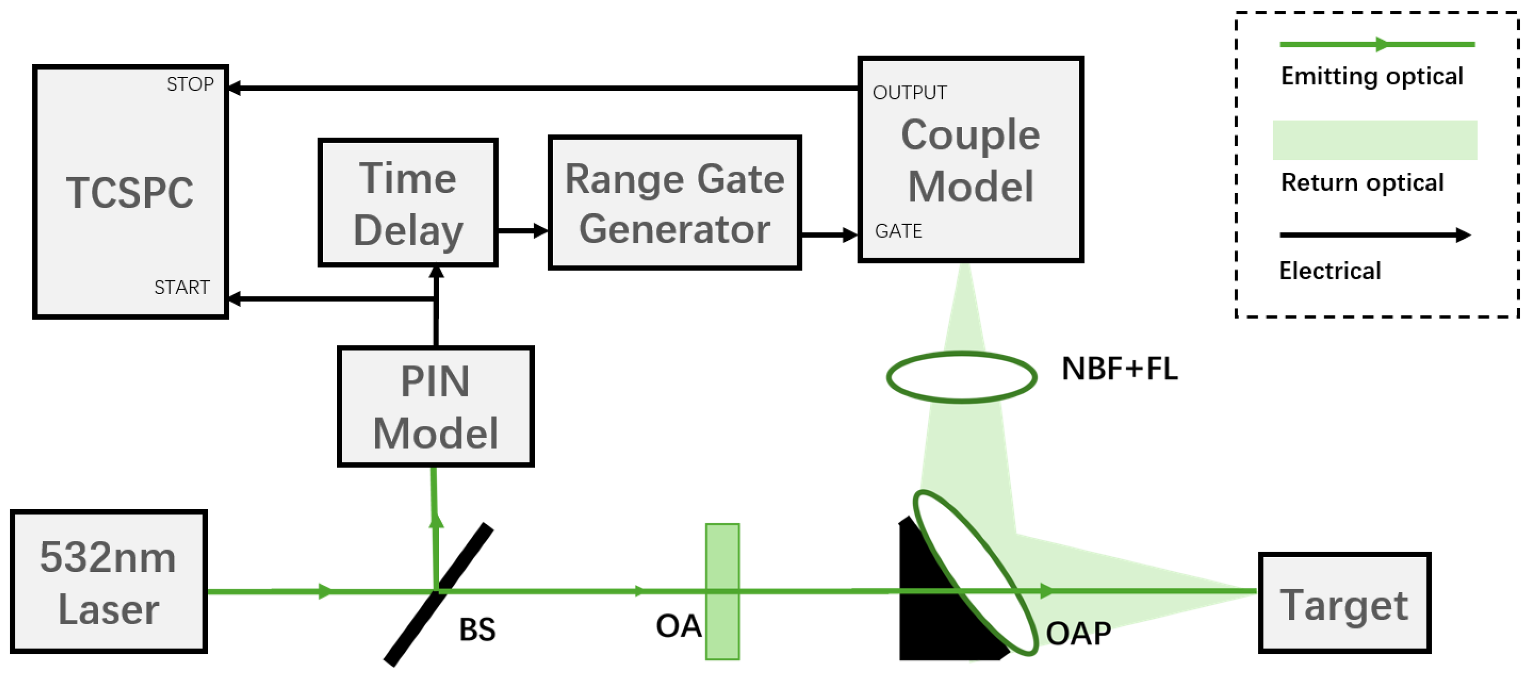
To obtain stable and reproducible first-photon statistics under photon-starved conditions, an underwater photon-counting LiDAR platform based on gated time-correlated single-photon counting (TCSPC) was developed, as shown in Figure 1. A 532 nm pulsed laser served as the illumination source. The emitted beam was first split by a 99:1 beamsplitter (BS), with the 1% reflected component directed onto a PIN photodiode. After pulse conditioning and waveform shaping, the photodiode output generated a TTL signal that served as the START synchronization signal of the system, thereby defining the temporal reference for each pulse repetition interval. The remaining optical energy was adjusted by an optical attenuator assembly (OA) and then delivered to the underwater target through a coaxial optical path formed around an off-axis parabolic mirror (OAP) with a central aperture. On the return path, the target echo retraced the same optical axis, passed through a narrowband filter (NBF) and a focusing lens (FL) to improve background rejection and optical coupling efficiency, and was finally recorded by a single-photon avalanche diode (SPAD). Following a preset delay referenced to the laser trigger, the range-gate generator issued the gating signal, thereby confining detection to the expected echo-arrival window, while the TCSPC module digitized the arrival time of the first detected event in each pulse repetition interval.

For clarity, the graphical conventions adopted in Figure 1 are explicitly defined here. The dark green lines and arrows denote the emitted optical path from the transmitter to the target, the light green denotes the reflected optical path returning from the target to the receiver, and the black lines denote the electrical interconnections used for synchronization, triggering, gating, and signal readout. This unified representation separates optical propagation from the electronic timing chain and allows the system architecture and operating principle to be interpreted more directly from the schematic.

A coaxial transmit–receive geometry was adopted to maximize echo-coupling efficiency and reduce range instability associated with alignment errors during underwater measurements. By combining temporal gating with narrowband spectral filtering, the system effectively suppresses invalid triggers caused by near-field backscatter, ambient illumination, and parasitic stray light before histogram accumulation. The SPAD operated in Geiger mode and recorded only the timestamp of the first trigger within each repetition interval; the arrival-time histogram was then reconstructed from a large ensemble of repeated cycles. This acquisition strategy is central to the present study because the resulting histogram directly reflects the first-photon statistics that govern range walk formation under low-flux conditions.

Experiments were conducted under static laboratory conditions in a 10 m transparent freshwater tank, with a true target distance of approximately 9.11 m. The hardware models and timing-related specifications employed in the error analysis are summarized in

Table 1. Hardware configuration and key timing-related specifications of the underwater gated TCSPC LiDAR.

Component	Model	Key Specification Used in This Work	Role in the Error Budget
Laser source	MPL-H-532 nm-30 μJ-CH80180	532 nm; 4 kHz operation; pulse width 1.388 ns; single-pulse energy 34.6 μJ; power stability 0.196%	Sets emitted waveform width and energy, thereby affecting echo width and $N_{pe}$.
Single-photon detector	SPD300A-PC SPAD	Spectral response 400–1100 nm; dead time ∼50 ns; dark count $< 100$ cps; timing jitter ∼624 ps; afterpulse 6.15%	First-photon triggering and detector dead time are part of the dominant RWE mechanism; timing jitter contributes to residual random error.
Time-to-digital converter	FT1040	4 parallel counting channels; histogram/time-tag resolution 16 ps; dead time $< 10$ ns; max event transfer rate 40 M Events/s	Determines quantization and timestamp precision in the readout chain.
Delay generator	ASG8100	Programmable delay gating for echo- window placement; ASG8000-series delay resolution 52 ps and RMS jitter $\le 35$ ps (series specification)	Sets the gate-zero reference and suppresses early backscatter; fixed common-mode offsets are largely cancelled by reference-plane differencing.

, whereas the principal acquisition parameters and environmental conditions are listed in

Table 2. Acquisition and environment settings used in the underwater validation experiments.

Parameter	Value	Notes
Water medium	Clear freshwater tank	Static laboratory condition; not intended to reproduce a full sea/lake environment.
Tank length	10 m	Indoor calibration/validation tank.
True target range	$\approx 9.11$ m	Validation range used for brick, stone, and acrylic targets.
Pulse repetition frequency	4 kHz	Synchronized with the TCSPC trigger chain.
Gate width	20 ns	Gate centered around the predicted echo arrival time.
Accumulated pulses per measurement	40,000	Integration time $=10$ s per histogram at 4 kHz.
Detector operating mode	Geiger-mode first-photon triggering	Only the first trigger in each laser pulse period is timestamped.
Low-photon fitting interval	$N_{pe}<1.6$	Working interval in which the linear approximation is calibrated.

.

In the present system, the laser pulse width primarily broadens the instrument response, the SPAD dead time participates in the physical formation of range walk error, and the TDC quantization together with the delay-generator jitter mainly contributes to the residual error budget after calibration. Because the subsequent correction is based on reference-plane differential calibration, most stable common-mode delays introduced by the trigger chain, cable routing, and TDC zero reference are largely cancelled and therefore are not expected to dominate the pre-correction centimeter-scale bias. A quantitative order-of-magnitude estimate derived from these specifications is provided later in Section 5.3.

4. Refined Range Walk Error Model for the Low-Photon Regime

Conventional RWE compensation often adopts a quadratic polynomial approximation of the RWE–$N_{pe}$ relationship. However, our experimental data indicate that, in the low-photon regime, the quadratic model effectively degenerates into an approximately linear function and its second-order term contributes negligibly. Therefore, for underwater low-photon operation (in this work typically $N_{pe}<1.6$), we construct an RWE model that is convenient for engineering implementation and present a reference-plane-based linear calibration procedure. Compared with free-space scenarios, underwater absorption and multiple scattering reshape the echo waveform (broadening and long tail) and significantly raise the background triggering rate within the gate, making first-photon triggering more susceptible to “noise-first” occlusion and to drift in water conditions. Accordingly, while retaining the interpretability of a linear model in the low-photon regime, we incorporate underwater-specific waveform asymmetry and background occlusion into the parameter estimation and calibration steps.

4.1. Linearization of the RWE–N_pe Relationship in the Low-Photon Regime

When $N_{pe}<1.6$ and the gate window is sufficiently short such that pile-up is not significant, $\mathrm{RWE}\left(N_{pe}\right)$ often exhibits an approximately linear dependence on $N_{pe}$. To obtain an analytic form that can be used for correction, the signal arrival rate is written as

$${\lambda }_s\left(t\right)=N_{pe} g\left(t\right), {\int }_0^{T_g}g\left(t\right) dt=1,$$

(11)

where $g\left(t\right)$ is the normalized temporal shape of the echo within the gate (including the system IRF and the scattering-induced broadening and tail). Let $G\left(t\right)={\int }_0^{t}g\left(u\right)du$ denote the cumulative signal shape, and define the cumulative background intensity as

$${\Lambda }_b\left(t\right)={\int }_0^t{\lambda }_b\left(u\right)du.$$

(12)

Using Equations (5), (6) and (8), the conditional mean first-trigger time can be expanded around $N_{pe}=0$ as

$$\overline{t}\left(N_{pe}\right)\approx {\overline{t}}_0+\kappa N_{pe}+O\left(N_{pe}^2\right),$$

(13)

where ${\overline{t}}_0$ is the mean first-detection time under background-only triggering. It is defined only when the background-only triggering event has a nonzero probability $P_0>0$:

$${\overline{t}}_0={\displaystyle \frac{1}{P_0}}{\int }_0^{T_g}t {\lambda }_b\left(t\right)e^{-{\Lambda }_b\left(t\right)}dt, P_0=1-e^{-{\Lambda }_b{T}_g}.$$

(14)

The first-order coefficient $\kappa$ quantifies the drift rate of the conditional mean trigger time as weak signal photons are injected. Retaining both the numerator expansion and the normalization term yields

$$\kappa ={\displaystyle \frac{1}{P_0}}{\int }_0^{T_g}(t-{\overline{t}}_0)[g\left(t\right)-{\lambda }_b\left(t\right)G\left(t\right)]e^{-{\Lambda }_b\left(t\right)}dt.$$

(15)

Substituting Equation (13) into Equations (9) and (10) yields the following approximately linear correction expression in the low-photon regime:

$$\mathrm{RWE}\left(N_{pe}\right)\approx a\left(c\right)N_{pe}+b\left(c\right), a\left(c\right)={\displaystyle \frac{c_w}{2}}\kappa \left(c\right), b\left(c\right)={\displaystyle \frac{c_w}{2}}[{\overline{t}}_0\left(c\right)-{\tau }_{\mathrm{true}}].$$

(16)

The notation $a\left(c\right)$ and $b\left(c\right)$ emphasizes that the fitted slope and intercept are condition-dependent parameters rather than universal constants. If water-condition changes only scale the echo amplitude while preserving the waveform shape $g\left(t\right)$ and the in-gate background level ${\lambda }_b$, the effect is largely absorbed by the measured $N_{pe}$. By contrast, if turbidity also changes pulse broadening, tailing, or the in-gate backscatter background, both the slope and the intercept migrate and the calibration should be updated.

To make the condition dependence more explicit when the water medium is parameterized by the beam-attenuation coefficient $c_{att}$, the signal primary-photoelectron term in Equation (16) may be factorized as

$$N_{pe}(c_{att},R)=K_0\rho \exp (-2c_{att}R) {\eta }_g(c_{att},R).$$

(17)

where $K_0$ absorbs the transmitted pulse energy, receiver geometry, optical throughput, and photoelectric efficiency; $\rho$ is the target reflectance at the operating wavelength; and ${\eta }_g(c_{att},R)$ denotes the gate-capture factor of the broadened underwater echo.

The waveform-shape term and the in-gate background term can then be written as

$$g(t;c_{att})={\displaystyle \frac{h_{\mathrm{EMG}} \left[t;\mu \left(c_{att}\right),\sigma \left(c_{att}\right),\tau \left(c_{att}\right)\right]}{{\int }_0^{T_g}{h}_{\mathrm{EMG}} \left[u;\mu \left(c_{att}\right),\sigma \left(c_{att}\right),\tau \left(c_{att}\right)\right] du}},$$

(18)

$${\lambda }_b\left(c_{att}\right)={\lambda }_{\mathrm{dark}}+{\lambda }_{\mathrm{amb}}+{\lambda }_{\mathrm{bs}}\left(c_{att}\right),$$

(19)

Accordingly, the first-order linear coefficients in Equation (16) may be interpreted as

$$a\left(c_{\mathrm{att}}\right)={\displaystyle \frac{c_w}{2}}\kappa \left(c_{\mathrm{att}}\right), b\left(c_{\mathrm{att}}\right)={\displaystyle \frac{c_w}{2}}[{\overline{t}}_0\left(c_{\mathrm{att}}\right)-{\tau }_{\mathrm{true}}]$$

(20)

It follows that if the water condition mainly rescales the echo amplitude through $\exp (-2c_{att}R)$ while leaving ${\eta }_g$, $g\left(t\right)$, and ${\lambda }_b$ nearly unchanged, the effect is largely absorbed by the measured $N_{pe}$ and the fitted RWE–$N_{pe}$ line changes little. By contrast, if $c_{att}$ also changes the EMG width $\sigma$, the scattering tail $\tau$, the gate-capture factor ${\eta }_g$, or the in-gate backscatter term ${\lambda }_{\mathrm{bs}}$, then both a and b migrate and the calibration should be updated. In the present clear-water tank experiment, $c_{att}$ is used as a compact descriptor of the water condition rather than as an independently inverted measurement variable.

4.2. Practical Estimation of RWE and N_pe in Underwater Low-Photon Data

To support modeling and correction of range walk error in underwater photon-counting LiDAR under low-photon conditions, this subsection describes the data acquisition and noise-processing pipeline. A characteristic of underwater data is that the target return is broadened and tailed by absorption and multiple scattering, while dark counts, ambient light, and backscatter introduce near-random noise triggers within the gate. The core challenge is that signal photons are concentrated in a narrow time interval, whereas background photons arrive quasi-randomly across the gate and can be of comparable magnitude. If statistics of the first-trigger time are computed over the entire gate, early noise triggers will systematically occlude the subsequent signal, biasing both the time-of-flight estimate and the photon-number estimate. We therefore adopted a two-stage “separate–estimate” procedure: the histogram was decomposed into signal-trigger and noise-trigger components, the noise-occlusion effect was explicitly compensated for, and the measured echo time and $N_{pe}$ were computed.

(1) Density-driven localization of the signal window. The gate was discretized into K time bins, and the histogram counts were denoted by $H\left[k\right]$. A sliding window of width w was used to compute the local sum $D\left[k\right]$ along the time axis. Bins satisfying $D\left[k\right]\ge \mu$ were treated as candidate signal bins and were then merged via connectivity to obtain the final signal interval.

$$D\left[k\right]=\sum _{i=k}^{k+w-1}H\left[i\right].$$

(21)

(2) Signal/noise decomposition and time-of-flight estimation. Let the signal interval start at bin l with length m, and denote the counts within the signal interval by $s_k$. To accommodate peak broadening due to scattering, we estimated the measured echo time using a weighted centroid:

$${\tau }_{\mathrm{mea}}=t_g+\Delta t\left[(l-1)+{\displaystyle \frac{{\sum }_{k=1}^m(k-\frac{1}{2})·s_k}{{\sum }_{k=1}^m{s}_k}}\right]$$

(22)

(3) Detection probability and $N_{pe}$ estimation (with noise-occlusion compensation). In a single exposure, N pulse repetition frequencies were accumulated. The signal-trigger probability was obtained by normalizing the total counts in the signal interval:

$$P_{\mathrm{sd}}={\displaystyle \frac{{\sum }_{k=1}^m{s}_k}{N}}={\displaystyle \frac{{\sum }_{k=1}^{l+m-1}H\left[k\right]}{N}}$$

(23)

Before the signal arrival, the noise-trigger probability in the leading interval was estimated, and the equivalent signal-trigger probability without occlusion was recovered accordingly:

$$P_{\mathrm{nd}}={\displaystyle \frac{{\sum }_{k=1}^{l-1}{n}_k}{N}}, P_{\mathrm{sd}}^{\mathrm{re}}={\displaystyle \frac{P_{\mathrm{sd}}}{1-P_{\mathrm{nd}}}}$$

(24)

Under the Poisson-arrival assumption, the mean number of signal primary photoelectrons within the gate is

$$N_{pe}=-\ln (1-P_{sd}^{re}).$$

(25)

Equation (24) must satisfy the physical interval $0\le P_{sd}^{re}<1$. When low counts or background-estimation uncertainty drive $P_{sd}^{re}$ outside that interval, the corresponding sample is treated as outside the valid working range of the estimator rather than being propagated into Equation (25). This practical restriction is now stated explicitly to avoid the nonphysical logarithm issue noted by the reviewers.

Because “noise-first triggering” is explicitly incorporated in the above estimator, it can preserve the cross-condition comparability of $N_{pe}$ even under strong backscatter. After estimating ${\tau }_{\mathrm{mea}}$ and $N_{pe}$, the subsequent RWE calibration and compensation models can be solved.

To obtain an arrival-rate expression that is numerically tractable and consistent with underwater echo morphology, the equivalent temporal response of the target return is modeled using an exponentially modified Gaussian (EMG), which can be interpreted physically as the convolution of “Gaussian system jitter” and an “exponential tail induced by underwater scattering” [23,24]:

$$h_{\mathrm{EMG}}\left(t\right)={\displaystyle \frac{A}{2\tau }}\exp \left[{\displaystyle \frac{{\sigma }^2}{2{\tau }^2}}-{\displaystyle \frac{t-\mu }{\tau }}\right]\mathrm{erfc}\left\{{\displaystyle \frac{1}{\sqrt{2}}}\left[{\displaystyle \frac{\sigma }{\tau }}-{\displaystyle \frac{t-\mu }{\sigma }}\right]\right\}.$$

(26)

where $\sigma$ reflects the combined effect of system jitter and underwater-propagation broadening, whereas $\tau$ characterizes the time scale of the scattering-induced long tail. In the low-photon regime, RWE varies approximately linearly and monotonically with $N_{pe}$, so a practical calibration model is written as

$$\Delta R \left(\mathrm{RWE}\right)\approx a{N}_{pe}+b, N_{pe}\le 1.6.$$

(27)

In Equation (27), the coefficient a primarily captures the sensitivity of first-photon triggering to leading-edge advancement and is jointly influenced by $\sigma$, $\tau$, and the background level. The intercept b absorbs fixed biases associated with the gate setting, reference definition, and any residual common-mode timing offset that survives the differential calibration.

4.3. Reference-Plane Differential Calibration and Linear Compensation

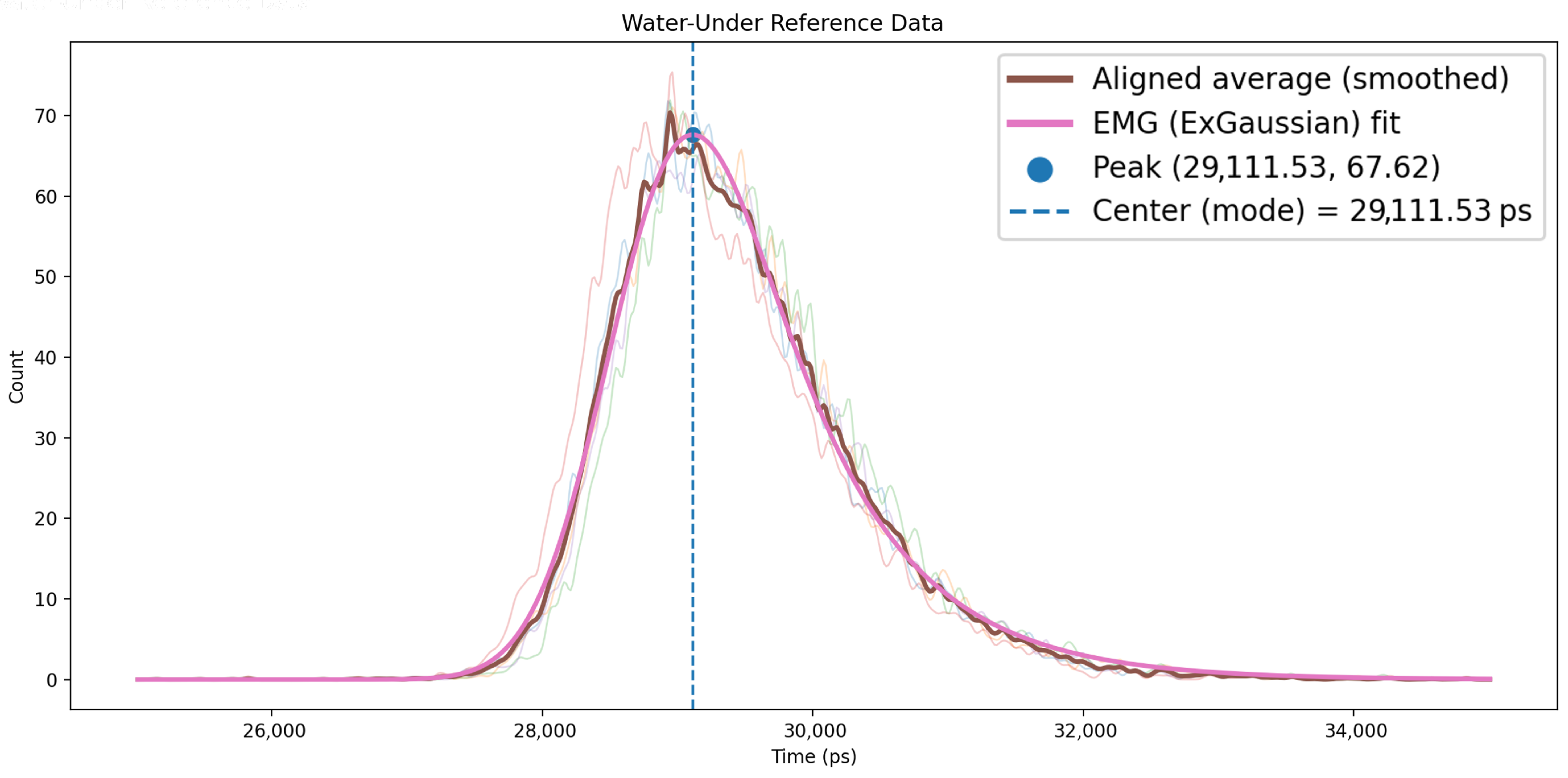
To obtain compensation parameters matched to a specific system–water condition, we adopted a differential calibration strategy using a reference plane and the target return. This strategy avoids dependence on absolute emission-time drift and explicitly reflects the influence of scattering-induced broadening on the estimated echo center in the fitting process. In the experiment, a high-reflectance white board was placed at the reference position to acquire histograms. Multiple measurements were peak-aligned and averaged to improve the signal-to-noise ratio; an EMG model was then fitted to the averaged echo to extract the mode time $t_{ref}$. Figure 2 shows the aligned-averaged histogram at the reference plane and the EMG fitting result. In this experiment, we obtained

$$t_{ref}=\mathrm{29,111.53} \mathrm{ps}.$$

(28)

The target plane was then moved to the ranging position ($R_{\mathrm{true}}=9.11$ m). Under the same water conditions, a set of echo datasets spanning the low-photon regime was collected by adjusting either the target reflectance or the transmitted power. For the i-th dataset, let $t_i$ denote the mode time of the target echo obtained from the EMG fit; the measured round-trip time difference is

$$\Delta {\tau }_{\mathrm{mea},i}=t_i-t_{ref}.$$

(29)

The geometric ground truth corresponds to a round-trip time difference of $\Delta {\tau }_{\mathrm{geo},\mathrm{ref}}$. Accordingly, the time-difference error and the range walk error are defined as

$$\Delta {\tau }_i=\Delta {\tau }_{\mathrm{mea},i}-\Delta {\tau }_{\mathrm{geo},\mathrm{ref}}, {\mathrm{RWE}}_i={\displaystyle \frac{c_w}{2}}·\Delta {\tau }_i$$

(30)

For all sample pairs $(N_{pe,i},{\mathrm{RWE}}_i)$ in the low-photon regime, Equation (27) was fitted via weighted least squares regression to obtain the linear compensation model under the current water condition. The weights are typically related to the peak counts or the fitting residuals so as to reduce the influence of low-count samples and outliers caused by abnormal scattering waveforms.

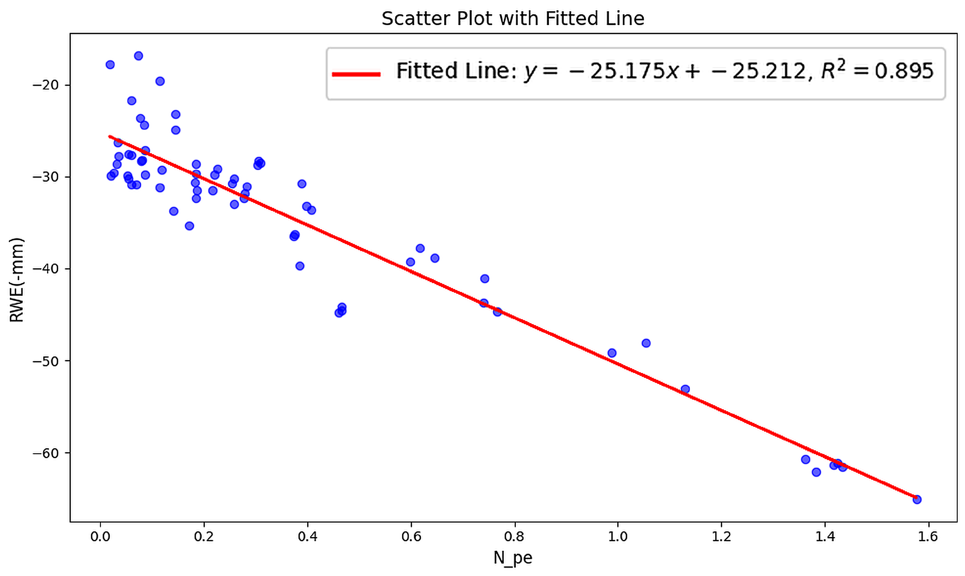
Figure 3 plots the scatter distribution of RWE versus the mean number of signal primary photoelectrons $N_{pe}$ at the target range of 9.11 m, together with the linear fit. The fitted linear model is

$$\mathrm{RWE}=-25.175 N_{pe}-25.212 \left(\mathrm{mm}\right).$$

(31)

The goodness-of-fit is $R^2=0.895$, indicating that within the low-photon-dominated regime of this experiment, the linear model captures the primary trend of systematic drift. However, the scatter is visibly larger in the very low-photon region because Poisson fluctuations, noise-first triggering, and EMG-fit uncertainty are even more evident there. Accordingly, the physical interpretation of this low-$N_{pe}$ heteroscedasticity is discussed further in Section 4.4.

4.4. Experimental Results and Comparison

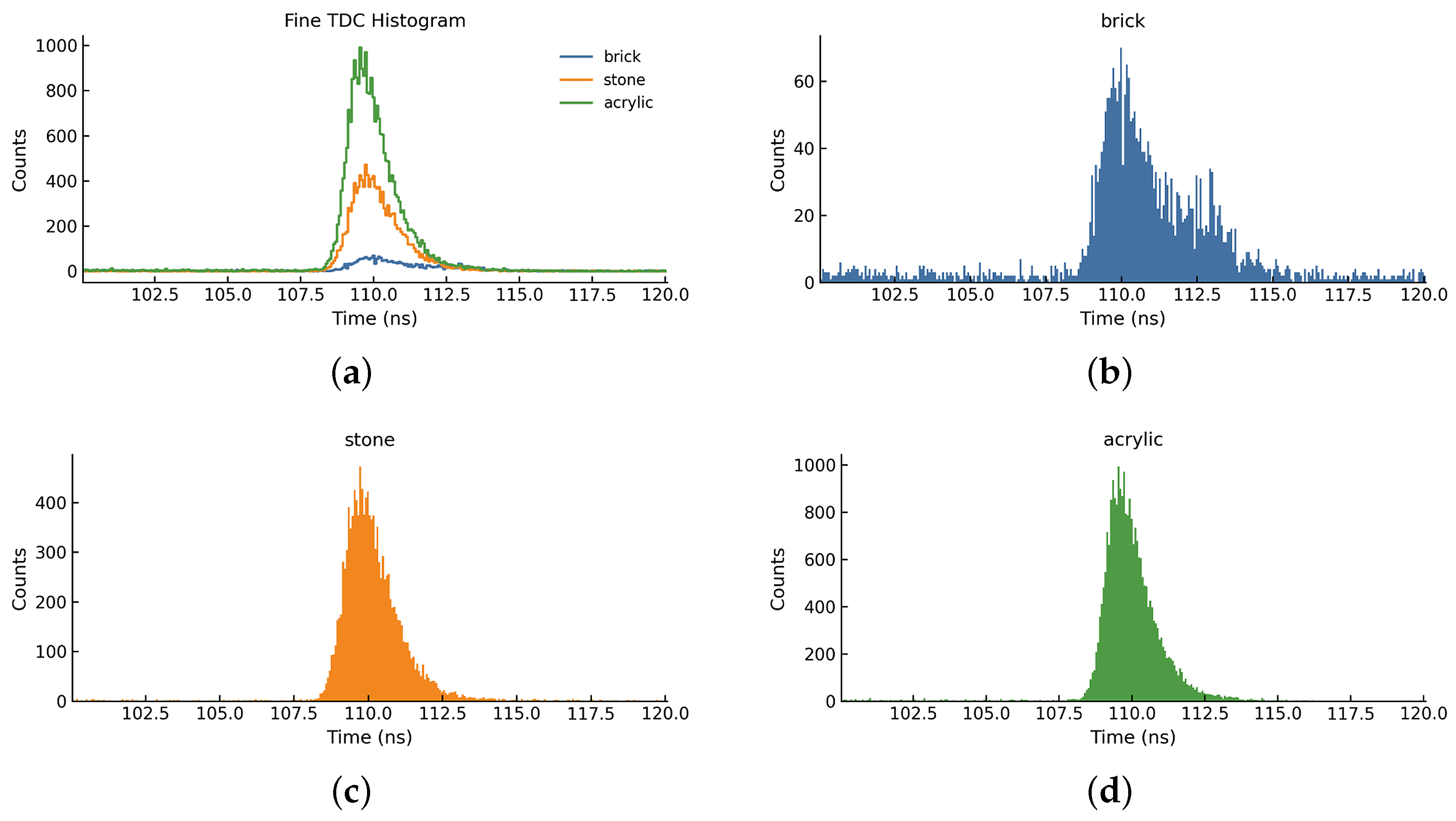
To validate Equation (31) in an underwater ranging scenario, we conducted experiments at a true range of 9.11 m using three targets with markedly different echo strengths (brick, stone, and acrylic). Under the same transmitted power and acquisition duration, arrival-time histograms were collected. The main return peak was fitted with an EMG model to estimate its central time, and $N_{pe}$ was estimated from histogram statistics.

Figure 4 shows the Fine-TDC histograms of the three targets and their overlay. The echo strengths differ substantially, with $N_{pe}$ values of 0.0695, 0.4081, and 1.1301 for brick, stone, and acrylic, respectively. As the echo becomes stronger, first-photon triggers tend to occur earlier on the rising edge, and the peak center shifts forward in time, leading to an underestimated flight time (and thus an underestimated range). This behavior is consistent with the SPAD “first-photon triggering + dead-time” mechanism.

Table 3. Ranging results at 9.11 m for different targets and performance of RWE correction.

Target	${\mathit{N}}_{\mathit{pe}}$	${\mathit{t}}_{\mathit{fit}}$ (ps)	Uncorrected Error $|{\mathbf{\Delta }}_1|$ (mm)	Estimated Linear Compensation (mm)	Residual After Linear Correction $|{\mathbf{\Delta }}_2|$ (mm)	Estimated Quadratic Compensation (mm)	Residual After Quadratic Correction $|{\mathbf{\Delta }}_3|$ (mm)
Brick	0.0695	109,814.55	30.911	26.962	3.949	2.674	28.237
Stone	0.4081	109,796.32	33.617	31.748	1.869	8.217	25.400
Acrylic	1.1301	109,617.41	53.089	53.662	0.573	24.551	28.538

${\Delta }_1$: Uncorrected ranging error; ${\Delta }_2$: Residual after linear correction; ${\Delta }_3$: Residual after quadratic correction. The linear correction reduces the mean error from 39.205 mm to 2.130 mm, achieving a 94.57% improvement over the uncorrected results and significantly outperforming the quadratic model.

reports that the uncorrected absolute ranging errors for brick, stone, and acrylic are 30.911 mm, 33.617 mm, and 53.089 mm, respectively. Moreover, the stronger the return (larger $N_{pe}$), the more pronounced the range underestimation, highlighting the systematic dependence of RWE on echo strength. Following the linear correction workflow in Section 4.3, the residual errors are reduced to 3.949 mm, 1.869 mm, and 0.573 mm. The mean absolute error decreases from 39.205 mm to 2.130 mm, corresponding to a 94.57% improvement in ranging accuracy. This millimeter-scale residual level remains compatible with the intended short-range high-precision underwater ranging task addressed in this paper.

For comparison, the quadratic model form commonly adopted in Ref. [8] yields residual errors of 24.288 mm, 25.400 mm, and 29.111 mm, with a mean error of 27.392 mm. These results demonstrate that, under the present low-photon condition ($N_{pe}<1.6$), the linear correction can stably compress RWE to the millimeter scale, achieving an order-of-magnitude improvement over the quadratic fit tuned for higher-photon operation, and showing excellent error suppression on the validation data.

The different corrected residuals for brick, stone, and acrylic do not imply that these materials intrinsically reduce RWE. Rather, the materials generate different $N_{pe}$ levels and slightly different waveform shapes because their reflectance and surface-scattering properties differ at 532 nm. The proposed linear compensation removes the dominant $N_{pe}$-dependent systematic bias, whereas small residual differences remain due to waveform-shape mismatch, background fluctuation, and fitting uncertainty at very low counts.

In summary, in underwater low-photon ranging experiments at a true range of 9.11 m, the systematic range walk error caused by variations in echo strength can be effectively characterized by $N_{pe}$. The linear compensation model established in Section 4.3 substantially reduces the ranging bias across different echo conditions, providing a more stable distance reference for subsequent 3D reconstruction and quantitative measurement.

5. Discussion

5.1. Relation to Existing Studies

The present paper does not claim that range walk is unique to underwater LiDAR. The underlying mechanism—first-photon triggering under finite detector dead time—is general to SPAD/TCSPC systems [16,17,18]. The underwater specificity lies in the calibration scenario because water attenuation, multiple scattering, and backscatter jointly modify signal amplitude, echo asymmetry, and background triggering inside the gate. Compared with the high-order prior-curve correction reported for underwater photon-counting imaging by Hua et al. [8], the present method focuses on the low-photon region and provides a simpler condition-calibrated linear mapping that is directly linked to measured $N_{pe}$. The reflectance- and stability-related error analyses reported for terrestrial LiDAR by Kelly et al. [21] and Cassanelli et al. [22] further support the need to separate systematic bias from random dispersion when evaluating ranging correction.

5.2. Portability and Practical Operating Window

In practice, when using this system to measure distances to underwater targets, water conditions generally remain relatively stable or fluctuate only slightly; in such cases, recalibration is not required for each measurement. However, if the water conditions change significantly, it would be reasonable to recalibrate the slope (a) and intercept (b), though this would not diminish the value of this study.

Therefore, the fitted coefficients (a) and (b) should be interpreted as system–water-condition parameters rather than as universal constants. If water-property changes only scale the echo amplitude, the influence is largely absorbed by measured $N_{pe}$. If turbidity also alters the waveform width $\sigma$, the scattering tail $\tau$, or the in-gate background ${\lambda }_b$, the calibration line shifts. Therefore, the current model is intended for repeated or accumulated TCSPC measurements under stable or slowly varying conditions. It is not presented as a single-shot correction for fast-moving, non-cooperative targets. The method remains valid as long as the signal window can be localized reliably, the leading-noise estimate does not dominate the gate, and the recovered trigger probability $P_{sd}^{re}$ stays inside the physical interval $[0, 1)$.

In practical deployment, the pre-calibration adopted here should be understood as a system–environment calibration step carried out at the beginning of an experiment or refreshed whenever the water condition changes appreciably. A reference target, a reference channel, or a periodically reacquired calibration sequence can be used to update $a\left(c_{att}\right)$ and $b\left(c_{att}\right)$. Accordingly, the present work demonstrates a laboratory-validated condition-calibrated workflow, whereas real-time turbidity-adaptive updating remains an important subject for future work.

5.3. Hardware Error Contribution and Order-of-Magnitude Estimate

The dominant uncorrected centimeter-level bias in this work originates from first-photon statistics coupled with SPAD dead time rather than from stable hardware timing offsets alone. To separate the dominant walk mechanism from auxiliary timing-chain limits, the measured timestamp can be decomposed as

$$t_{\mathrm{meas}}=t_{\mathrm{FP}}(N_{pe},{\lambda }_b,g)+{\delta }_{\mathrm{sys}}+{\epsilon }_{\mathrm{hw}}.$$

(32)

After reference-plane differencing, most common-mode fixed offsets are canceled, and the measured range error can be written as

$$\Delta R_{\mathrm{meas}}=\Delta R_{\mathrm{rw}}+\Delta R_{\mathrm{sys},\mathrm{res}}+{\epsilon }_{R,\mathrm{hw}}.$$

(33)

For an order-of-magnitude estimate, the residual hardware-related random timing term is approximated by

$${\sigma }_{t,\mathrm{hw}}^2\approx {\sigma }_{\mathrm{SPAD}}^2+{\sigma }_{\mathrm{TDC},q}^2+{\sigma }_{\mathrm{ASG}}^2+{\sigma }_{\mathrm{sync}}^2, {\sigma }_{\mathrm{TDC},q}\approx {\displaystyle \frac{\Delta t_{\mathrm{bin}}}{\sqrt{12}}}.$$

(34)

$${\sigma }_{R,\mathrm{hw}}\approx {\displaystyle \frac{(c_w/2) {\sigma }_{t,\mathrm{hw}}}{\sqrt{N_{\Sigma }}}}, N_{\Sigma }\approx N_{pe}N.$$

(35)

where $N_{\Sigma }$ denotes the order-of-magnitude accumulated signal-primary-photoelectron count in the calibration histogram. In the present experiments, $N=\mathrm{40,000}$. Using the detector-report timing jitter of 624 ps, the FT1040 time-bin width of 16 ps, and the ASG8100-series delay-generator RMS jitter of at most 35 ps,

Table 4. Order-of-magnitude estimate of hardware-induced random ranging uncertainty in the present 9.11 m experiment.

Target	Mean ${\mathit{N}}_{\mathit{pe}}$	Approx. Accumulated Signal Primary Photoelectrons ${\mathit{N}}_{\mathbf{\Sigma }}$	${\mathit{\sigma }}_{\mathit{R},\mathbf{hw}}$ (mm), Optimistic 624 ps as FWHM	${\mathit{\sigma }}_{\mathit{R},\mathbf{hw}}$ (mm), Conservative 624 ps as RMS
Brick	0.0695	2780	0.57	1.34
Stone	0.4081	16,324	0.24	0.55
Acrylic	1.1301	45,204	0.14	0.33

gives an order-of-magnitude estimate under two interpretations of the detector report: an optimistic case in which 624 ps is treated as a FWHM value and a conservative case in which 624 ps is treated directly as an RMS value. We adopted a moderate 20–40 ps contribution for this estimate.

Table 4 shows that the estimated hardware-induced random ranging uncertainty is approximately 0.14–0.57 mm in the optimistic interpretation and 0.33–1.34 mm in the conservative interpretation. These values are substantially smaller than the uncorrected centimeter-level RWE observed experimentally (mean absolute error 39.205 mm). Therefore, stable hardware timing offsets do not alter the main physical conclusion of the present study: the dominant pre-correction bias is the first-photon statistical walk coupled with SPAD dead time, whereas hardware-related timing terms mainly enter the corrected residual budget.

5.4. Limitations

The validation was conducted in a static freshwater tank, rather than under controlled turbidity, flow rate, or aeration conditions, or in a field deployment environment. Moving forward, I will use the findings and experience gained from this experiment to conduct comprehensive validation in marine or lake environments and to perform additional experiments under varying turbidity conditions.

6. Conclusions

This work addresses the modeling and compensation of range walk error in underwater gated TCSPC photon-counting LiDAR under conditions of strong backscatter and waveform broadening in the low-photon regime. Based on first-photon triggering statistics, we establish a mapping between RWE and the mean number of signal primary photoelectrons $N_{pe}$ and develop a linear correction framework that adapts to water conditions. The main conclusions are as follows:

1.

Within a non-homogeneous Poisson first-arrival framework, we jointly consider echo broadening/long-tail formation due to underwater propagation, background triggering within the gate, and the “noise-first occlusion” effect. A computable expression for RWE is derived and a linearized approximation for the low-photon regime is obtained, providing a unified modeling framework for quantitative evaluation and portable compensation of underwater RWE across scenarios.

2.

For histogram data in which weak signals coexist with strong background underwater, we construct a data-processing pipeline of “signal-window localization–signal/noise decomposition–noise-occlusion compensation” and provide robust estimators for the echo center time and $N_{pe}$. By explicitly compensating for the noise-trigger probability $P_{nd}$, the method maintains the cross-condition comparability of $N_{pe}$ when backscatter increases, laying a data foundation for subsequent calibration and correction.

3.

We propose a linear compensation procedure centered on reference-plane differential calibration. In underwater ranging experiments at a true range of 9.11 m, brick/stone/acrylic yield $N_{pe}$ values of 0.0695, 0.4081, and 1.1301, with uncorrected errors ${\Delta }_1$ of 30.911 mm, 33.617 mm, and 53.089 mm. After applying the proposed linear compensation, the corrected errors ${\Delta }_2$ decrease to 3.949 mm, 1.869 mm, and 0.573 mm, respectively; the mean error is reduced from 39.205 mm to 2.130 mm (94.57% improvement). Compared with the quadratic compensation model (mean error 27.392 mm), the proposed method achieves millimeter-level error compression under underwater low-photon conditions, verifying its practical effectiveness.

Although the proposed method demonstrates strong error suppression and promising transferability in underwater low-photon ranging experiments, several directions merit further study. Future work may proceed as follows:

1.

Echo-shape parameter estimation: extend single-peak fitting to an EMG or multi-component deconvolution framework to more accurately characterize the long-tail structure induced by strong scattering, and to improve robustness under high turbidity and non-single-peak returns.

2.

Online calibration coupled with water-parameter estimation: leveraging synchronized observations from multi-channel SPAD arrays or reference channels, explore joint estimation and rapid updating mechanisms for water optical parameters (e.g., attenuation coefficient and backscatter strength), thereby improving real-time performance and cross-scenario adaptability.