Polarization Control Methods for Mitigating Four-Wave Mixing Effect in NG-EPON Networks

Abstract

In order to meet the growing traffic demands, the formulation of the NG-EPON protocol is under heated discussion. Therefore, for the wavelength allocation scheme of NG-EPON, adopting O-band wavelengths is considered as the potentially feasible solution. While the low dispersion property of O-band would induce four-wave mixing (FWM) to NG-EPON networks. In this paper, polarization control methods are used to mitigate the FWM effect in NG-EPON networks, including orthogonal linear polarization, circular polarization and left to right circular polarization alternation methods. For the 4-channel NG-EPON networks, the FWM-induced sensitivity penalty is achieved as 0.3 dB by using the orthogonal linear polarization method, compared with the FWM-induced sensitivity penalty of 4.1 dB, which is the worst-case scenario. By adopting the circular polarization method, the FWM-induced sensitivity penalty is measured as 0.2 dB, which is 3.9 dB better than that of the worst-case scenario. By employing the left to right circular polarization alternation method, the FWM-induced sensitivity penalty is 0.2 dB, compared with the worst-case scenario, whose sensitivity penalty is 4.1 dB induced by the FWM. In addition, for the 8-channel NG-EPON networks, the FWM-induced sensitivity penalty is decreased to 0.4 dB for minimum, compared with the worst-case scenario, whose sensitivity penalty is unpredictable.

1. Introduction

With the rapid adoption of new services like cloud computing, big data, ultra-high-definition video services, high-definition video conferencing, etc., industry and academia must continue to research into higher performance network facilities to meet the user traffic demands. Passive optical network (PON) is widely used and has established itself as a standard solution for access networks because of its wide geographic coverage, low cost, and high capacity [1]. Therefore, EPON [2], GPON [3], 10G-EPON [4], XG(S)-PON [5] and other technologies [6,7] can provide high speed bandwidth access services for users. However, due to the rising user demands for network bandwidth and the rapid development of new services, the outdated PON technology cannot support the large bandwidth requirements of the next generation services. Therefore, in order to achieve the continued upgradation of PON technology, next generation Ethernet passive optical network (NG-EPON) technology is proposed. NG-EPON is standardized by IEEE 802.3ca and it can provide multiple wavelengths for transmission, with each wavelength offering a transmission rate of 25 Gb/s [8]. By adopting multiple-wavelength multiplexing technology on the basis of time division multiplexing, a single optical network unit (ONU) can be equipped with multiple transceivers, which greatly increases the transmission rate of the ONU.

Although multi-wavelength transmission of NG-EPON has greatly improved the capacity of optical access networks, it also suffers from the four-wave mixing (FWM) effect induced by O-band wavelength allocation [9,10]. As an effective and low-complexity solution, polarization control has been widely concerned in FWM suppression of O-band WDM systems in recent years. K. Inoue proposed that orthogonal polarization arrangement of signals can effectively suppress FWM in multichannel transmission [11], laying a theoretical foundation for polarization-based FWM mitigation. Recent relevant studies have further explored polarization effects in O-band WDM transmission. T. Kurosu verified that polarization management and specific polarization arrangements (e.g., xyxy and xyyx) can suppress FWM in O-band WDM systems [12]. M. Bendaoud analyzed polarization-dependent impairments and optimized polarization modulation parameters to improve O-band WDM transmission performance [13]. Y. Yan proposed polarization-regulating devices applicable to O-band WDM systems, though not targeting FWM suppression [14]. While these studies either focus on general O-band WDM systems rather than NG-EPON, they only propose simple polarization arrangements without systematic schemes, or do not target NG-EPON-specific FWM needs. Thus, a targeted, systematic polarization control method is urgently required to solve FWM problems in O-band NG-EPON networks.

In this paper, polarization control methods are applied to NG-EPON networks for mitigating the FWM effect, where orthogonal linear polarization, circular polarization and left to right circular polarization alternation methods are adopted. When the NG-EPON networks have four channels and the orthogonal linear polarization method is used, the sensitivity improvement is calculated as 3.8 dB. When circular polarization method is applied, a 3.9 dB sensitivity improvement is obtained. When left to right circular polarization alternation method is employed, the sensitivity improvement is measured as 3.9 dB. When the NG-EPON networks have eight channels, the sensitivity penalty is reduced to a minimum of 0.4 dB by using the polarization control methods, compared with the unpredictable sensitivity penalty after the same polarization transmission (the worst-case scenario).

2. Theoretical Analysis

The essence of FWM is a third-order nonlinear optical effect, and its physical origin lies in the third-order nonlinear polarization intensity ($P^{\left(3\right)}$) generated when a strong light field interacts with a medium. According to the theory of nonlinear optics, for isotropic media (such as optical fibers, certain semiconductor materials), the polarization intensity ($\overrightarrow{P}$) of a medium can be expanded as the sum of linear and nonlinear terms in powers of the field strength [10]:

$$\overrightarrow{P}={\overrightarrow{P}}^{\left(1\right)}+{\overrightarrow{P}}^{\left(2\right)}+{\overrightarrow{P}}^{\left(3\right)}+\cdots$$

(1)

where ${\overrightarrow{P}}^{\left(1\right)}={\epsilon }_0{\chi }^{\left(1\right)}·\overrightarrow{E}$ is the linear polarization term, ${\chi }^{\left(1\right)}$ is the first-order linear polarization tensor, ${\epsilon }_0$ is the vacuum dielectric constant. ${\overrightarrow{P}}^{\left(2\right)}$ is the second-order nonlinear polarization term existing only in anisotropic media (such as crystals). In isotropic media, ${\chi }^{\left(2\right)}=0$ due to its symmetry. Therefore, in scenarios such as optical fibers, ${\overrightarrow{P}}^{\left(2\right)}$ can be disregarded. ${\overrightarrow{P}}^{\left(3\right)}$ is the third-order nonlinear polarization term, which is the main source of FWM. Its expression is determined by the product of the third-order polarization tensor ${\chi }^{\left(3\right)}$ and the light field.

In the FWM process, three incident pump/signal light fields (${\omega }_1,{\omega }_2, {\omega }_3$) interact with the medium, resulting in the generation of a new mixed field (${\omega }_4$). And the mixing field ${\omega }_4$ of FWM is excited by the component (${\overrightarrow{P}}^{\left(3\right)}({\omega }_4)$) of the third-order nonlinear polarization intensity with a frequency of ${\omega }_4$, which can be expressed as follows [11]

$${\overrightarrow{P}}_j^{\left(3\right)}\left({\omega }_4\right)={\displaystyle \frac{1}{4}}{\epsilon }_0{\sum }_{l,m,n}{{\chi }^{\left(3\right)}}_{jlmn}({\omega }_4;{\omega }_1,{\omega }_2,-{\omega }_3)E_{l0}({\omega }_1)E_{m0}({\omega }_2)E_{n0}^{\ast }({\omega }_3)e^{i(\overrightarrow{k_1}+\overrightarrow{k_2}-\overrightarrow{k_3})}$$

(2)

where j, l, m, n refers the Cartesian coordinate component, ${{\chi }^{\left(3\right)}}_{jlmn}({\omega }_4;{\omega }_1,{\omega }_2,-{\omega }_3)$ means the third-order polarization tensor, $E_{l0}\left({\omega }_1\right)$, $E_{m0}\left({\omega }_2\right)$ and $E_{n0}^{\ast }\left({\omega }_3\right)$ denote the complex amplitude of the light field (including polarization information), $\ast$ means co-adjoint, $\overrightarrow{k_1}$, $\overrightarrow{k_2}$ and $\overrightarrow{k_3}$ are the wave vectors of the light fields.

For isotropic media such as optical fibers and glass, ${{\chi }^{\left(3\right)}}_{jlmn}$ has a high degree of symmetry. Furthermore, if the incident light is linearly polarized light and the polarization direction is in the transverse plane (x-y plane), two orthogonal linearly polarized basis vectors can be defined as $\widehat{x}$ (horizontal polarization) and $\widehat{y}$ (vertical polarization). Then, ${{\chi }^{\left(3\right)}}_{jlmn}$ can be simplified to two scalar parameters

$${{\chi }^{\left(3\right)}}_{xxxx}={{\chi }^{\left(3\right)}}_{yyyy}={{\chi }^{\left(3\right)}}_{zzzz}={\chi }_1$$

(3)

$${{\chi }^{\left(3\right)}}_{xxyy}={{\chi }^{\left(3\right)}}_{yyxx}={{\chi }^{\left(3\right)}}_{xyxy}={{{\chi }^{\left(3\right)}}_{yxyx}=\chi }_2$$

(4)

where ${\chi }_1$ is the third-order polarization rate in the same polarization direction, and ${\chi }_2$ denotes the third-order polarization rate with crossed polarization directions. According to the results of nonlinear optics, in isotropic media, ${\chi }_1$ and ${\chi }_2$ satisfy the relationship of ${\chi }_2={\displaystyle \frac{{\chi }_1}{2}}$.

Assuming the polarization unit vectors of the three incident fields are respectively $\widehat{e_1}$, $\widehat{e_2}$ and $\widehat{e_3}$ (all are within the x-y plane), then its complex amplitude can be expressed as $\overrightarrow{E_{i0}}=E_{i0}\widehat{e_i}$ ($E_{i0}$ is a scalar amplitude). After substituting $\overrightarrow{E_{i0}}$ into ${\overrightarrow{P}}_j^{\left(3\right)}\left({\omega }_4\right)$ and expanding it, the scalar form of the FWM polarization intensity amplitude (only retaining the components related to the mixed-frequency field) can be obtained

$$P_{FWM}={\displaystyle \frac{1}{4}}{\epsilon }_0{\chi }_{eff}^{\left(3\right)}{E}_{10}{E}_{20}{E}_{30}^{\ast }$$

(5)

where ${\chi }_{eff}^{\left(3\right)}$ is the effective third-order polarization rate. It is the core parameter that determines the intensity of FWM, and its value is directly dependent on the polarization state of the incident field, which can be written as

$$\begin{gathered} {\chi }_{eff}^{\left(3\right)}={\chi }_1\left(\widehat{e_1}·\widehat{e_4}\right)\left(\widehat{e_1}·\widehat{e_3^{\ast }}\right)\left(\widehat{e_2}·\widehat{e_4}\right)\left(\widehat{e_2}·\widehat{e_3^{\ast }}\right) \\ \hspace{1em}\hspace{1em}\hspace{1em}\hspace{1em}\hspace{1em}\hspace{1em}\hspace{1em}\hspace{1em}\hspace{1em}\hspace{1em}\hspace{1em}\hspace{1em}\hspace{1em}\hspace{1em}\hspace{1em}\hspace{1em}\hspace{1em}\hspace{1em}+2{\chi }_2\left[\left(\widehat{e_1}·\widehat{e_4}\right)\left(\widehat{e_2}·\widehat{e_3^{\ast }}\right)\left(\widehat{e_1}·\widehat{e_3^{\ast }}\right)\left(\widehat{e_2}·\widehat{e_4}\right)\right] \end{gathered}$$

(6)

To further simplify, consider the collinear FWM scenario (such as in optical communication where the signal and the pump propagate in the same direction). In this case, the polarization direction of the mixed field ($\widehat{e_4}$) is related to the polarization direction of the incident field, and momentum conservation is automatically satisfied ($\overrightarrow{k_4}\approx \overrightarrow{k_1}+\overrightarrow{k_2}-\overrightarrow{k_3}$). Therefore, $\widehat{e_4}$ can be approximately regarded as being parallel to the incident field polarization. At this point, ${\chi }_{eff}^{\left(3\right)}$ can be simplified as

$${\chi }_{eff}^{\left(3\right)}={(\widehat{e_p}·\widehat{e_s})}^2·{\displaystyle \frac{3}{2}}{\chi }_1$$

(7)

It can be seen that, the ${\chi }_{eff}^{\left(3\right)}$ is proportional to the square of the dot product of the incident field’s polarization unit vector. The dot product ($\widehat{e_p}·\widehat{e_s}$) describes the degree of polarization overlap between the two fields, which is the core physical essence of polarization control to suppress FWM.

Based on the above-mentioned relationship between ${\chi }_{eff}^{\left(3\right)}$ and polarization, the suppression effects of FWM in the cases of orthogonal linear polarization and circular polarization are respectively derived.

It is assumed that the polarization direction of the pump light is $\widehat{x}$ and the polarization direction of the signal light is $\widehat{y}$ (i.e., orthogonal linear polarization). Then, the pump polarization unit vector $\widehat{e_p}=(1,0)$ (x direction) and the signal polarization unit vector $\widehat{e_s}=(0,1)$ (y direction). The dot product of two orthogonal linearly polarized fields is written as [15]

$$(\widehat{e_p}·\widehat{e_s}) \left(1,0\right)· \left(0,1\right)=0$$

(8)

The output intensity of FWM ($I_{FWM}$) is proportional to the square of ${\chi }_{eff}^{\left(3\right)}$, i.e., $I_{FWM} \propto {\left|{\chi }_{eff}^{\left(3\right)}\right|}^2={\left|{\left(\widehat{e_p}·\widehat{e_s}\right)}^2·{\displaystyle \frac{3}{2}}{\chi }_1\right|}^2=0$. It can be seen that orthogonal linear polarization ensures that the polarization of the pump and the signal are completely uncorrelated (with a dot product of 0), resulting in an effective third-order polarization of 0 and complete suppression of FWM (in an ideal scenario).

Circularly polarized light can be decomposed into two orthogonal linearly polarized components. The polarization unit vectors of these components need to be described in complex form. They can be defined as

$$\widehat{e_L}={\displaystyle \frac{1}{\sqrt{2}}}(\widehat{x}+i\widehat{y})$$

(9)

$$\widehat{e_R}={\displaystyle \frac{1}{\sqrt{2}}}(\widehat{x}-i\widehat{y})$$

(10)

where $\widehat{e_L}$ and $\widehat{e_R}$ denote the left-handed circular polarization and right-handed circular polarization, respectively. Assume that the pump light is left-circularly polarized, and the signal light is right-circularly polarized, then $\widehat{e_p}·\widehat{e_s}=\widehat{e_L}·\widehat{e_R^{\ast }}={\displaystyle \frac{1}{\sqrt{2}}}\left(\widehat{x}+i\widehat{y}\right)·{\displaystyle \frac{1}{\sqrt{2}}}\left(\widehat{x}+i\widehat{y}\right)={\displaystyle \frac{1}{2}}(\widehat{x}·\widehat{x}+i\widehat{x}·\widehat{y}+i\widehat{y}·\widehat{x}+i^2\widehat{y}·\widehat{y})$. Due to that $\widehat{x}·\widehat{x}=\widehat{y}·\widehat{y}=1$, $\widehat{x}·\widehat{y}=0$ and $i^2=-1$, $\widehat{e_p}·\widehat{e_s}=0$ and $I_{FWM}=0$. It can be seen that the polarization overlap degree of left-handed and right-handed circularly polarized light is 0 (the dot product is 0). Its essence lies in the orthogonality of the phases of circular polarization: the phase of the y-component of left-handed circular polarization leads that of right-handed circular polarization by π (equivalent to inversion), resulting in the cancelation of the contributions of nonlinear interactions, and ultimately FWM is suppressed.

3. Simulation Setup

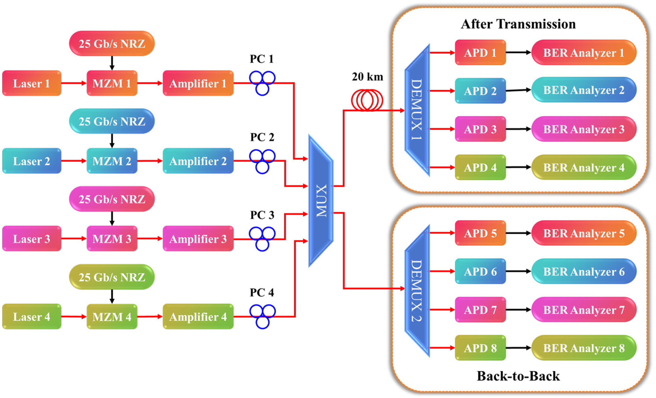
In order to investigate the effect of polarization control methods on mitigating the FWM effect, simulation systems are setup as shown in Figure 1 and all simulations are carried out by using the software of VPI Transmission Maker (Version 9.8). The employed parameters are given in

Table 1. Simulation parameters for investigating the FWM effect in NG-EPON networks.

Parameters	Value
Wavelengths	1294.57 nm, 1299.06 nm, 1303.58 nm, 1308.13 nm
Channel Spacing	200 GHz, 400 GHz, 800 GHz
Modulation Rate	25 Gb/s
Fiber Attenuation	0.34 dB/km
MUX and DEMUX Insertion Loss	1.5 dB
Chirp Coefficient	0
Out Power	8 dBm/channel
APD Dark Current	20 nA
Fiber Length	20 km
Zero-dispersion Wavelength	1303.58 nm
Dispersion Slope	0.093 ps/(nm2·km)
PMD coefficient	0.1 ps/km1/2
Extinction Ratio	10 dB
Nonlinear Refractive Index	2.6 × 10−20 m2/W
Core Area	80 × 10−12 m2

. At the transmitter side, four lasers operating at 1294.57 nm, 1299.06 nm, 1303.58 nm and 1308.13 nm are used as the optical carriers, where the channel spacing is 800 GHz. Note that, for improving the spectrum utilization, the channel spacing is also chosen as 400 GHz and 200 GHz [16]. Then, the Mach–Zehnder Modulators (MZMs) are utilized for modulating the 25 Gb/s non-return-to-zero (NRZ) electrical signals on the optical carriers, where the chirp coefficient and extinction ratio of the MZMs are 0 and 10 dB, respectively. After modulation, the signals are amplified to 8 dBm per channel by the amplifier models defined by VPI with fixed gain shape, which can act as the gain-controlled, power-controlled, or saturable amplifier, and limiting effects related to high output power or high gain are taken into account. Subsequently, the amplified signals are sent into the polarization controllers (PCs) for polarization control. Here, linear polarization (obtaining the most severe FWM) [17], orthogonal linear polarization, circular polarization and left to right circular polarization alternation states are set. For the orthogonal linear polarization method, if Channel 3 (Ch3) is set as the reference channel whose polarization angle is 0°, the polarization angle of Ch2 shall be 90°. And the polarization angle of Ch1 turns back to 0° for keeping a relatively orthogonal status. For the circular polarization method, the polarization state of all the channels is set as left circularly polarized. For the left to right circular polarization alternation method, if Ch3 is set as the reference channel whose polarization state is left circularly polarized, the polarization state of Ch2 shall be right circularly polarized. And the polarization state of Ch1 turns back to left circular polarization. In addition, considering the effects from the random rotation of the polarization states for different wavelengths caused by the standard single-mode fiber (SSMF) which is defined by the VPI software, the polarization states of all the channels shall be different during the real simulation. After polarization control, the signals are injected into a multiplexer (MUX) for coupling, whose insertion loss is 1.5 dB. Afterwards, the coupled signal is sent into a 20 km SSMF (meets SMF-28 parameter standards) for transmission, where the SSMF attenuation is 0.34 dB/km, the dispersion slope is 0.093 ps/(nm²·km) and the polarization mode dispersion (PMD) coefficient is 0.1 ps/km^1/2. Note that, due to the FWM effect which is closely related to the zero-dispersion wavelength of fiber [18], the zero-dispersion wavelength is set as 1303.58 nm (coincides with Ch3) for maximizing the FWM effect. After transmission, the coupled signal is de-multiplexed by a de-multiplexer (DEMUX) with an insertion loss of 1.5 dB. At the receiver side, the filtered signals are injected into the avalanche photodiodes (APDs) with a dark current of 20 nA and finally captured by the BER Analyzer modules for BER calculation. Furthermore, for achieving higher transmission capacity, the 8-channel NG-EPON system is also considered. Due to its similarity to the 4-channel system above-mentioned, the system description is omitted here.

4. Simulation Results and Analysis

4.1. The Obtained Results by Using Orthogonal Linear Polarization Method

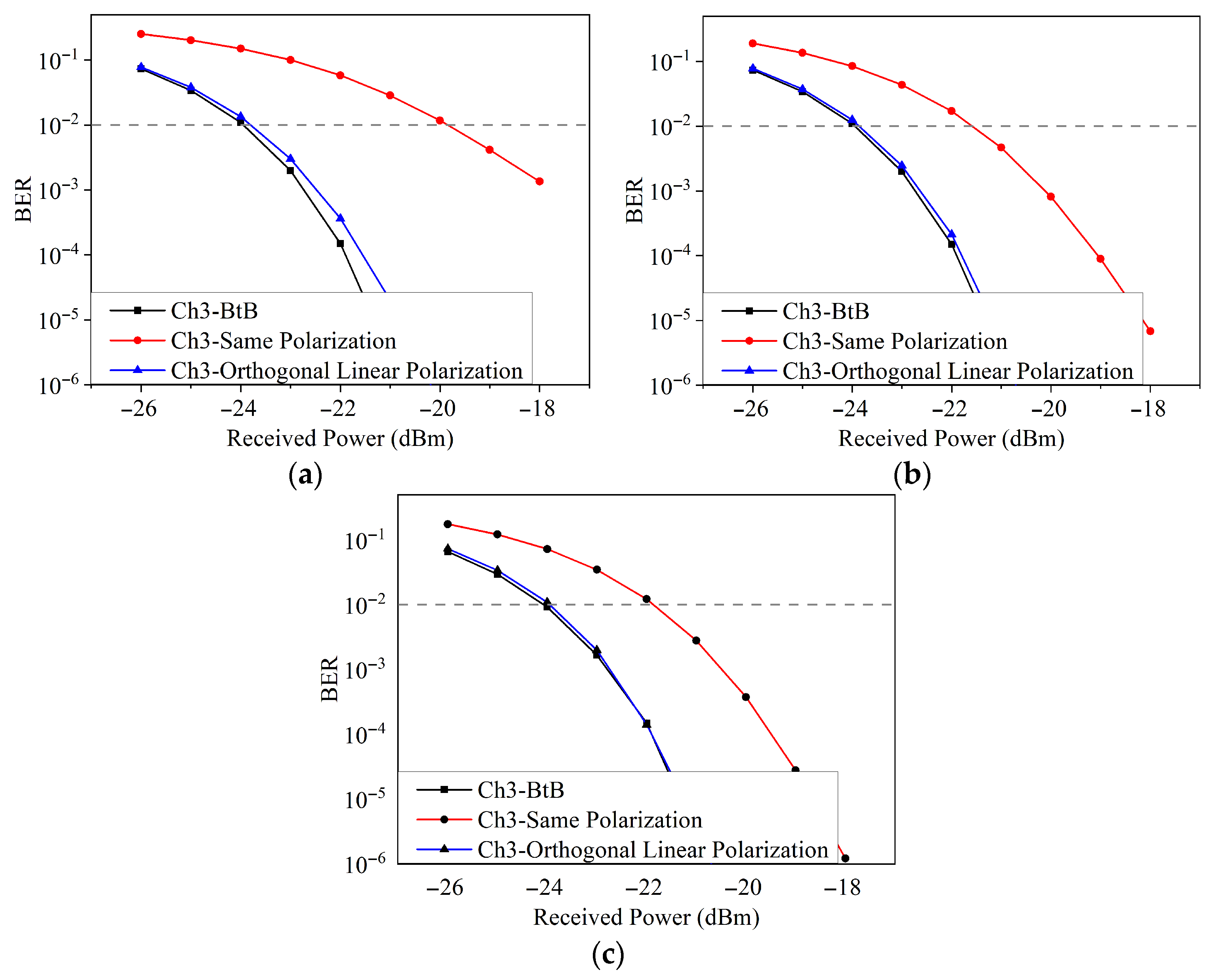
The optical fiber experiences the most severe FWM effect due to Ch3 which coincides with the optical fiber’s zero-dispersion wavelength. Therefore, the measured BER curves of Ch3 by using orthogonal linear polarization method are given as an illustration in Figure 2. Furthermore, Figure 2a represents the obtained BER curves of Ch3 when the channel spacing is 200 GHz. It can be seen that when the channels are transmitted after back-to-back (BtB), the achieved sensitivity of Ch3 is −24 dBm under the condition of 1 × 10⁻² BER threshold [19]. When the channels are transmitted after 20 km optical fiber under the same polarization condition, the obtained sensitivity of Ch3 is −19.9 dBm, i.e., the FWM-induced sensitivity penalty is 4.1 dB. While, by adopting the orthogonal linear polarization method, the obtained sensitivity of Ch3 is −23.7 dBm, i.e., the FWM-induced sensitivity penalty is substantially reduced to 0.3 dB. It is because of this that, by using the orthogonal linear polarization method, the efficiency of FWM has decreased significantly, which is explained in the theoretical part, thus achieving a 3.8 dB sensitivity improvement. Note that the theoretical analysis correctly deduces that the effective third-order susceptibility (${\chi }_{eff}^{\left(3\right)}$) becomes zero for ideally orthogonal polarizations (both linear and circular). While, in reality, due to the polarization crosstalk (e.g., PMD) there will be a slight residual intensity of FWM. Figure 2b illustrates the acquired BER curves of Ch3 when the channel spacing is 400 GHz. It can be seen that, with the increase in the channel spacing, the FWM-induced sensitivity penalty is reduced to 2.3 dB when the channels are transmitted under the same polarization. While, by utilizing the orthogonal linear polarization method, the FWM-induced sensitivity penalty is 0.1 dB, which is 2.2 dB better than that of the same polarization transmission scenario. Figure 2c depicts the achieved BER curves of Ch3 when the channel spacing is 800 GHz. It indicates that the FWM-induced sensitivity penalty can be ignored by employing the orthogonal linear polarization method, compared with the same polarization transmission case (the FWM-induced sensitivity penalty is 2.1 dB).

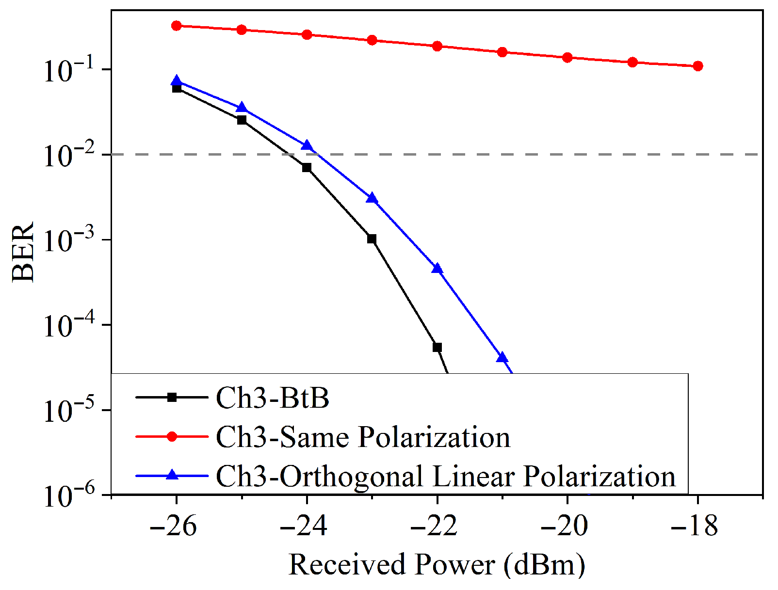
When the number of channels is increased to eight, the FWM effect becomes more severe because more wavelengths are involved in the FWM process. Here, the most severe case is represented as an example in Figure 3 when the channel spacing is 200 GHz. It can be seen that, after 20 km optical fiber transmission under the condition of same polarization, the BER of Ch3 cannot reach the BER thresholds, resulting in the unpredictable sensitivity penalty. While, by adopting the orthogonal linear polarization method, the FWM-induced sensitivity penalty is decreased to 0.5 dB.

4.2. The Obtained Results by Using Circular Polarization Method

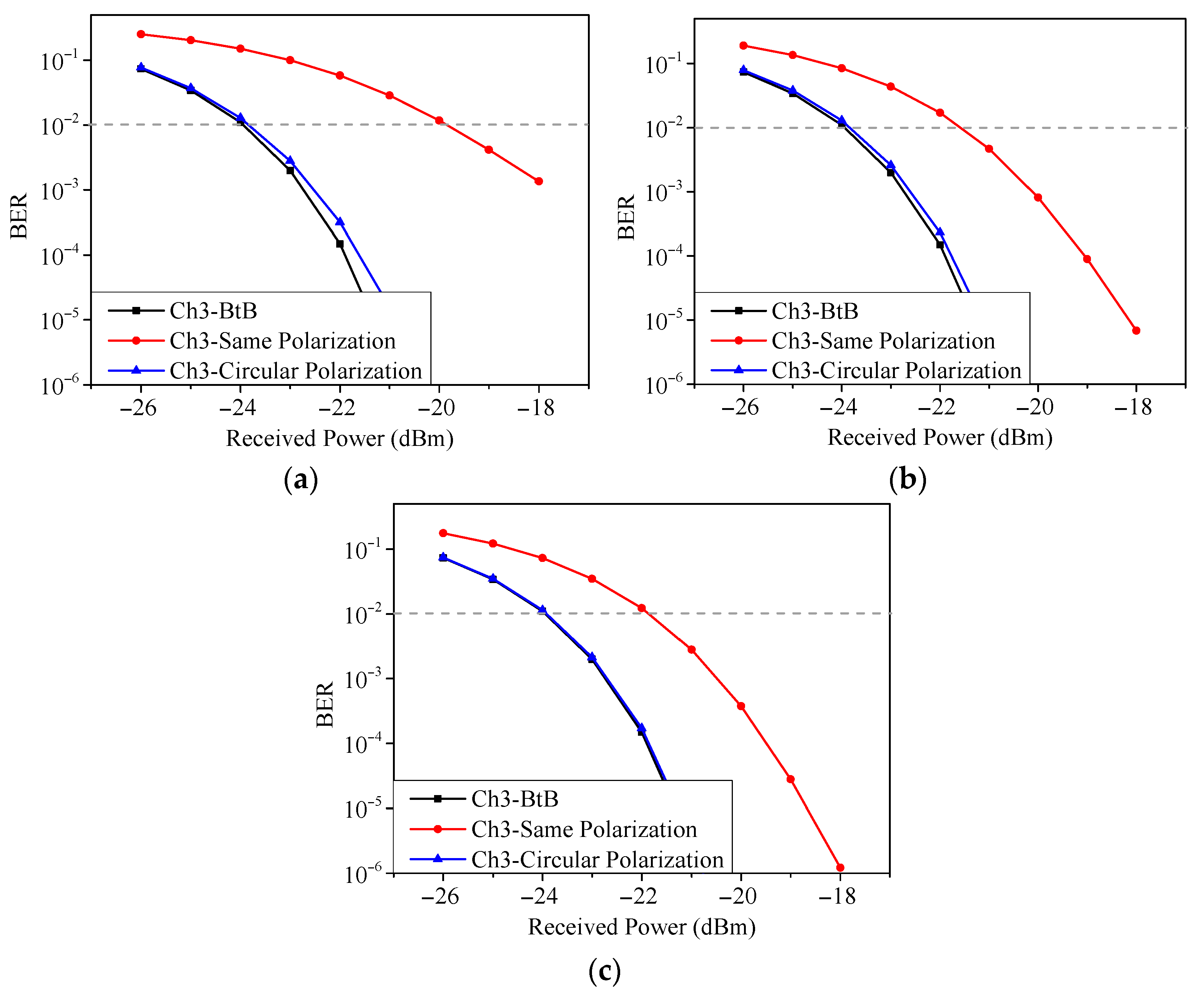
In order to explore BER further, the measured BER curves of Ch3 by using the circular polarization method are represented in Figure 4. Similar to the obtained results above-mentioned, the achieved sensitivities of Ch3 are −24 dBm and −19.9 dBm after BtB and the same polarization transmissions, respectively, when the channel spacing is 200 GHz, i.e., the FWM-induced sensitivity penalty is 4.1 dB. However, when the circular polarization method is used, the acquired sensitivity penalty is 0.2 dB, which is 3.9 dB better than that of the same polarization transmission case as given in Figure 4a. This is because when the circular polarization method is adopted, the interaction of adjacent pulses is lower and thus leads to the reduction in FWM efficiency. With the increase in the channel spacing to 400 GHz, the FWM-induced sensitivity penalty is 2.3 dB when the channels are transmitted after the same polarization transmission. While, by employing a circular polarization method, a 2.2 dB sensitivity improvement is achieved. From Figure 4c, it can be seen that the FWM-induced sensitivity penalty can be ignored when the channels are transmitted under the condition of circular polarization (i.e., the obtained BER curves of BtB and left to right circular polarization alternation method coincide).

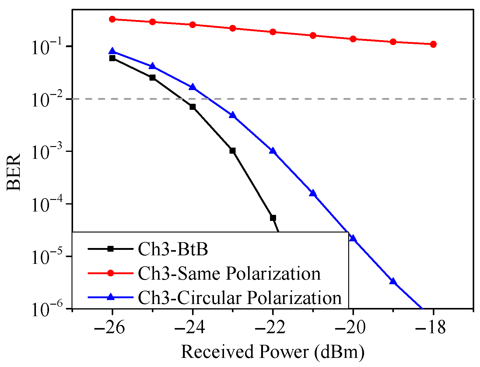
Figure 5 gives the BER curves of Ch3 when the channels are transmitted after BtB with the same polarization and circular polarization transmission. It can be seen that, with the use of the circular polarization method, the FWM-induced sensitivity penalty is reduced to 0.6 dB, compared with the unpredictable sensitivity penalty, which is the most severe case.

4.3. The Obtained Results by Using Left to Right Circular Polarization Alternation Method

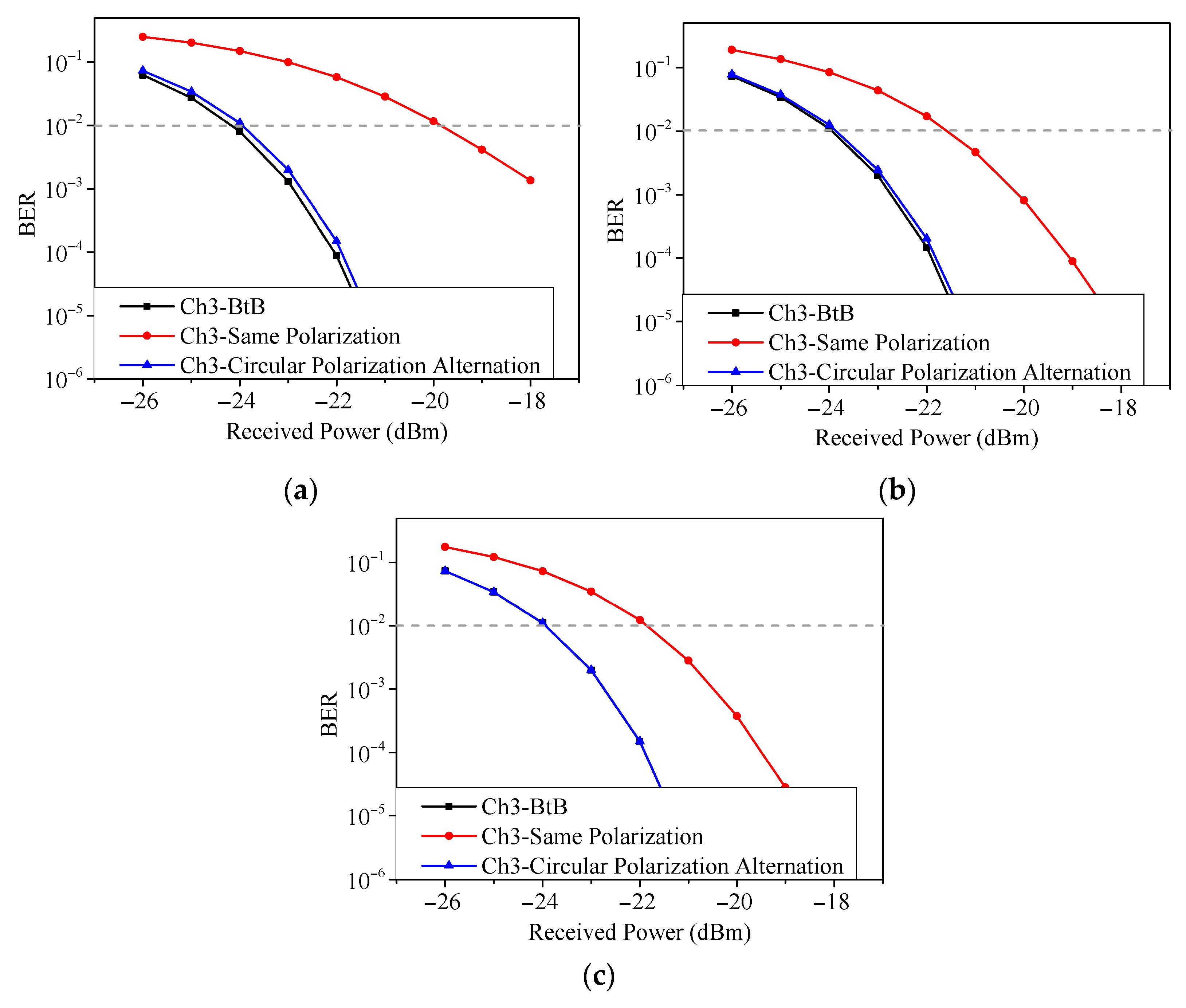
Finally, Figure 6 depicts the measured BER curves of Ch3 by using the left to right circular polarization alternation method when the channel spacing is 200/400/800 GHz. Therefore, Figure 6a shows the BER curves of Ch3 when the channel spacing is 200 GHz. It can be seen that when the channels are transmitted after 20 km optical fiber under the condition of same polarization, the FWM-induced sensitivity penalty is 4.1 dB. While, by utilizing the left to right circular polarization alternation method, a 0.2 dB sensitivity penalty is obtained, i.e., the sensitivity improvement is 3.9 dB through the use of the left to right circular polarization alternation method. When the channel spacing is increased to 400 GHz, a sensitivity improvement of 2.2 dB can be achieved. It can be demonstrated that the FWM-induced sensitivity penalty can be disregarded as the channel spacing is increased to 800 GHz (i.e., the obtained BER curves of BtB and left to right circular polarization alternation method coincide).

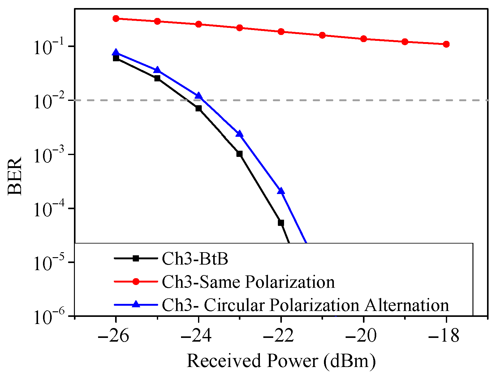
Figure 7 elucidated that when the channel spacing is 200 GHz and the number of channels is 8, the FWM-induced sensitivity penalty is decreased to 0.4 dB by using the left to right circular polarization alternation method, compared with the same polarization transmission case.

To better verify the effectiveness of the proposed scheme, several recently published studies for mitigating the FWM effect are cited for comparison [20,21] considering the simplicity of implementation in a typical WDM-based transmission system. The results demonstrate that the performance improvement achieved in this work is more pronounced relative to those reported in the literature. In future work, hybrid schemes that integrate multiple techniques will be explore to more effectively mitigate the FWM effect in NG-EPON.

5. Conclusions

In this paper, orthogonal linear polarization, circular polarization and left to right circular polarization alternation methods are employed to mitigate the FWM effect in NG-EPON. When there are four channels in NG-EPON, the orthogonal linear polarization method lowers the FWM-induced sensitivity penalty to 0.3 dB, which is 3.8 dB better than that of the same polarization case. By adopting a circular polarization method, a 3.9 dB sensitivity improvement is obtained. By employing a left to right circular polarization alternation method, the sensitivity improvement is 3.9 dB. In comparison to the unpredictable sensitivity penalty following the same polarization transmission, the sensitivity penalty can be minimized to 0.4 dB when the number of channels is 8. The acquired simulation results illustrate that the methods used as mentioned above show remarkable effect in FWM suppression. They contribute to the enhancement of NG-EPON system’s loss budget and in turn facilitate the improvement of network throughput and the extension of transmission distance, which could provide effective contribution for planning the NG-EPON standardization.

References

1. Xu, Y.; Wang, S.; Saleem, A. Simulative analysis of stimulated Raman scattering effects on WDM-PON based 5G fronthaul networks. Sensors 2025, 25, 3237. [Google Scholar] [CrossRef] [PubMed]
2. Memon, K.; Jaffer, S.; Qureshi, M.; Qureshi, K.K. Dynamic bandwidth allocation in time division multiplexed passive optical networks: A dual-standard analysis of ITU-T and IEEE standard algorithms. Peerj Comput. Sci. 2025, 11, e2863. [Google Scholar] [CrossRef] [PubMed]
3. Lu, J.; Fu, J.; Li, X.; Liang, Y. Innovative hard isolation techniques in GPON for modern power distribution networks. IEEE Access 2024, 12, 196637–196646. [Google Scholar] [CrossRef]
4. Houtsma, V.; van Veen, D. A study of options for high-speed TDM-PON beyond 10G. J. Lightwave Technol. 2017, 35, 1059–1066. [Google Scholar] [CrossRef]
5. Effenberger, F. The XG-PON system: Cost effective 10 Gb/s access. J. Lightwave Technol. 2011, 29, 403–409. [Google Scholar] [CrossRef]
6. Kumari, M. Design of long-reach symmetric 1.6 Tbps bidirectional NG-PON2 using 2D spectral/spatial SWZCC code. Microw. Opt. Technol. Lett. 2022, 65, 1822–1828. [Google Scholar] [CrossRef]
7. Kumari, M.; Arya, V. A smooth evolution of wavelength complement coding integrated MDM/coherent NGPON incorporating probabilistically shaped-512 QAM. Opt. Quantum Electron. 2024, 56, 82. [Google Scholar] [CrossRef]
8. Xu, Y.; Saleem, A. Investigation of stimulated Raman scattering effect on designing of NG-EPON systems. Opt. Eng. 2021, 60, 126101. [Google Scholar] [CrossRef]
9. Wu, X.; Li, Z.; Song, Y.; Guo, Y.; Yin, Y.; Wang, M. A novel wavelength plan for FWM suppression in NG-EPON. Opt. Commun. 2017, 403, 335–340. [Google Scholar] [CrossRef]
10. Agrawal, G.P. Nonlinear Fiber Optics, 5th ed.; Elsevier: Rochester, NY, USA, 2013. [Google Scholar]
11. Inoue, K. Arrangement of orthogonal polarized signals for suppressing fiber four-wave mixing in optical ultichannel transmission systems. IEEE Photonics Technol. Lett. 1991, 3, 560–563. [Google Scholar] [CrossRef]
12. Kurosu, T.; Suda, S.; Amano, T. Mitigation of Four-Wave Mixing by Means of Polarization Management in the O-Band. In Proceedings of the 2023 International Conference on Photonics in Switching and Computing (PSC), Mantova, Italy, 26–29 September 2023. [Google Scholar]
13. Bendaoud, M.; Imam, A.; Ghnimi, S.; Gharsallah, A. Dual-Polarization Quadrupling Generation for RoF-DWDM Transmission Using OCS with Dual-Parallel DD-MZM Under Nonlinear Effects. Res. Sq. 2025. [Google Scholar] [CrossRef]
14. Yan, Y.; Wu, Y.; Wang, Y.; Li, J.; Hu, J.; Wang, X. Deep-learning-based polarization-dependent switching metasurface in dual-band for optical communication. Nanophotonics 2025, 14, 5141–5152. [Google Scholar] [CrossRef] [PubMed]
15. Zilian, A.; Wright, J. Polarization effects in four-wave mixing of isotropic samples. Mol. Phys. 1996, 87, 1261–1271. [Google Scholar] [CrossRef]
16. Song, Y.; Yu, P.; Xu, Y.; Li, Z. Simulation and experimental investigation of nonlinear effects in 5G fronthaul transmission system based on WDM-PON architecture. Opt. Fiber Technol. 2021, 65, 102628. [Google Scholar] [CrossRef]
17. Wang, D.; Cheng, T.; Yeo, Y.; Xu, Z.; Wang, Y.; Xiao, G.; Liu, J. Performance comparison of using SOA and HNLF as FWM medium in a wavelength multicasting scheme with reduced polarization sensitivity. J. Light. Technol. 2010, 28, 3497–3505. [Google Scholar] [CrossRef]
18. Cai, P.; Gao, L.; Wu, Q.; Liu, A.; Long, Y.; Dai, S.; Li, Y.; Chen, Y.; Chen, L.; Huang, L.; et al. Experimental verification of polarization destabilization in vector four-wave mixing excited by dissipative solitons with wavelength-resolved polarizations. J. Light. Technol. 2024, 43, 2774–2781. [Google Scholar] [CrossRef]
19. Tao, M.; Zheng, J.; Dong, X.; Zhang, K.; Zhou, L.; Zeng, H.; Luo, Y.; Li, S.; Liu, X. Improved dispersion tolerance for 50G-PON downstream transmission via receiver-side equalization. In Proceedings of the 2019 Optical Fiber Communication Conference (OFC), San Diego, CA, USA, 3–7 March 2019; Optica Publishing Group: Washington, DC, USA, 2019; pp. 1–3. [Google Scholar]
20. Kurosu, R.; Kurosu, T.; Suda, S.; Amano, T. Inter-channel FWM mitigation using low-complexity digital pre-compensation for O-band IMDD transmission. In Proceedings of the 2025 Optical Fiber Communications Conference and Exhibition (OFC), San Francisco, CA, USA, 30 March–3 April 2025; IEEE: New York, NY, USA, 2025; p. W1E.3. [Google Scholar]
21. Saleem, A.; Xu, Y.; Wang, S. Research of fiber nonlinear effects in WDM-PON based 5G fronthaul networks. J. Nonlinear Opt. Phys. Mater. 2023, 32, 2350018. [Google Scholar] [CrossRef]
Figure 1. Simulation setup for investigating the effect of polarization control methods on mitigating the FWM effect.
Photonics 13 00419 g001
Figure 2. The measured BER curves of Ch3 after BtB; same polarization and orthogonal linear polarization transmission when the channel spacing is (a) 200 GHz (b) 400 GHz and (c) 800 GHz.
Photonics 13 00419 g002
Figure 3. The measured BER curves of Ch3 after BtB; same polarization and orthogonal linear polarization transmission when the channel spacing is 200 GHz and the number of channels is 8.
Photonics 13 00419 g003
Figure 4. The measured BER curves of Ch3 after BtB; same polarization and circular polarization transmission when the channel spacing is (a) 200 GHz (b) 400 GHz and (c) 800 GHz.
Photonics 13 00419 g004
Figure 5. The measured BER curves of Ch3 after BtB; same polarization and circular polarization transmission when the channel spacing is 200 GHz and the number of channels is 8.
Photonics 13 00419 g005
Figure 6. The measured BER curves of Ch3 after BtB; same polarization and left to right circular polarization alternation transmission when the channel spacing is (a) 200 GHz (b) 400 GHz and (c) 800 GHz.
Photonics 13 00419 g006
Figure 7. The measured BER curves of Ch3 after BtB; same polarization and left to right circular polarization alternation transmission when the channel spacing is 200 GHz and the number of channels is 8.
Photonics 13 00419 g007