Tip–Tilt Aberration Compensation for Laser Array Atmospheric Propagation Based on Cooperative Beacons

Abstract

Laser beam combining is essential for achieving high-power and high-radiance output. However, atmospheric turbulence induces independent tip–tilt aberrations across discrete sub-beams in laser array systems, which severely degrades the concentration of far-field energy. Traditional wavefront sensing techniques are primarily designed for the continuous wavefront of a single laser and are not directly applicable to laser array, whereas indirect optimization-based methods often suffer from slow convergence and limited real-time performance. To address these limitations, this study introduces a tip–tilt aberration compensation system for laser array propagation based on cooperative beacons with a shared-aperture transmit–receive configuration. The primary innovation consists of a modified Shack–Hartmann wavefront sensor (SHWFS) tailored to a discrete multi-beam layout, which facilitates the direct, independent, and simultaneous measurement of tip–tilt aberrations for each sub-beam. In conjunction with a segmented deformable mirror (SDM), the architecture can facilitate real-time closed-loop correction with high bandwidth and high precision. Numerical simulations of a 7-, 19-, and 37-beam laser array, together with validation experiments utilizing a 30-beam configuration, demonstrate that the proposed approach effectively suppresses tip–tilt error induced by turbulence. After closed-loop correction, the Strehl ratio (SR) increases above 0.92 ($r_0=5\mathrm{cm}$), while the beam quality factor β reduces below 1.37 ($r_0=5\mathrm{cm}$). Furthermore, the system retains performance stability as the number of sub-beams increases, demonstrating the scalability of the proposed method. In contrast to conventional approaches designed for a continuous wavefront, the proposed method offers a feasible approach for a discrete laser array system, providing robust and scalable tip–tilt correction under varying atmospheric conditions.

1. Introduction

High-energy laser (HEL) systems have attracted significant attention in applications such as directed energy, free-space optical communication, and long-distance power delivery. The advancement of HEL systems is primarily driven by the pursuit of increased output power and enhanced beam quality [1,2,3]. However, due to factors such as thermal effects, nonlinear effects, and component performance limits, it is difficult to further increase the power of a single laser while maintaining high beam quality once a certain threshold is reached [3]. Laser beam combining has consequently emerged as an effective approach to address these limitations and realize high-power, high-radiance output [4,5,6].

In practical scenarios, laser propagation is inevitably subject to atmospheric turbulence, which induces random wavefront distortions and significantly degrades both beam quality and energy concentration at the target [5,6,7]. These effects are more pronounced in laser array systems, in which multiple sub-beams propagate simultaneously and are independently affected by turbulence, leading to beam spreading, pointing errors, and a reduction in combining efficiency [6]. Adaptive optics (AO) has been widely utilized to correct turbulence-induced aberrations in both single-beam and multi-beam laser systems. AO in laser systems can facilitate real-time wavefront detection and correction effectively, reducing the impact of atmospheric turbulence and ensuring the performance of the system [8,9]. According to the Kolmogorov turbulence model, low-order aberrations dominate the total wavefront aberration. Specifically, tip–tilt aberration accounts for approximately 87% of the phase variance (after removing the piston term) [10]. Consequently, the effective compensation of tip–tilt aberration is essential for the improvement of the far-field beam quality of laser arrays.

Current methods for the correction of tip–tilt aberrations in laser array systems are generally classified into: indirect optimization-based methods and direct wavefront sensing methods. Indirect approaches, such as stochastic parallel gradient descent (SPGD) and associated optimization algorithms, employ far-field performance metrics (e.g., power or intensity) as feedback signals and iteratively refine control parameters to enhance beam quality [11,12,13,14,15]. Although these techniques offer flexibility and do not necessitate explicit wavefront sensors, they are typically characterized by slow convergence rates, high computational requirements, and constrained real-time performance.

In contrast, direct wavefront sensing methods utilize wavefront sensors such as Shack–Hartmann wavefront sensors (SHWFSs) to provide a more efficient approach by directly measuring tip–tilt aberration of each sub-beam and facilitating closed-loop correction [16,17,18]. These methods have been extensively utilized in adaptive optics systems owing to their high bandwidth, rapid response, and compatibility with established control algorithms. However, the traditional SHWFS is primarily designed for continuous wavefront and apertures. It is not inherently suitable for laser array systems characterized by discrete sub-beam and sub-aperture distributions. Furthermore, the independent and simultaneous measurement of tip–tilt aberrations for multiple sub-beams remains a significant challenge, especially under strong turbulence conditions.

Since this study focuses on detecting and correcting tip–tilt aberrations introduced by atmospheric turbulence using cooperative beacons, the research method is applicable to laser array with different combining methods and gain media. Therefore, multiple laser beams obtained by coherent or incoherent combining are collectively referred to as “laser array” in this paper.

Beacon-based wavefront sensing has long served as a fundamental methodology in AO systems, such as laser guide stars, and is used for the characterization of atmospheric turbulence along the propagation path. Specifically, the return light from a beacon effectively carries information regarding turbulence-induced wavefront distortions, thereby facilitating wavefront compensation at the transmitter. Although cooperative and non-cooperative beacon techniques have been extensively investigated and implemented in single laser systems, the application of these methods within laser array systems remains under-explored. In particular, the adaptation of beacon-based wavefront sensing to discrete multi-aperture configurations, in which the independent tip–tilt aberrations of multiple sub-beams must be measured and corrected simultaneously, introduces significant technical complexities. Furthermore, the integration of cooperative beacon-based wavefront sensing with the shared-aperture transmit–receive architecture for laser array system still remains insufficiently investigated.

To address these challenges, this paper develops a tip–tilt aberration compensation system for laser array propagation based on cooperative beacons with a shared-aperture transmit–receive telescope. To measure the tip–tilt aberration of each sub-beam in the laser array, a modified SHWFS is proposed to address the discrete nature of laser array, enabling independent and direct tip–tilt measurement for each sub-beam. Simultaneously, a segmented deformable mirror (SDM), with sub-mirrors corresponding to the sub-beams, is utilized to implement real-time closed-loop correction for each sub-beam.

The proposed approach is validated through both numerical simulations and a principle verification experiment. The results demonstrate that the system effectively suppresses the tip–tilt aberration induced by atmospheric turbulence and significantly enhances the far-field beam quality and energy concentration. Additionally, the proposed method demonstrates robustness under varying turbulence conditions and exhibits scalability across diverse array configurations.

2. Principles and Methods

2.1. Array Laser System Model

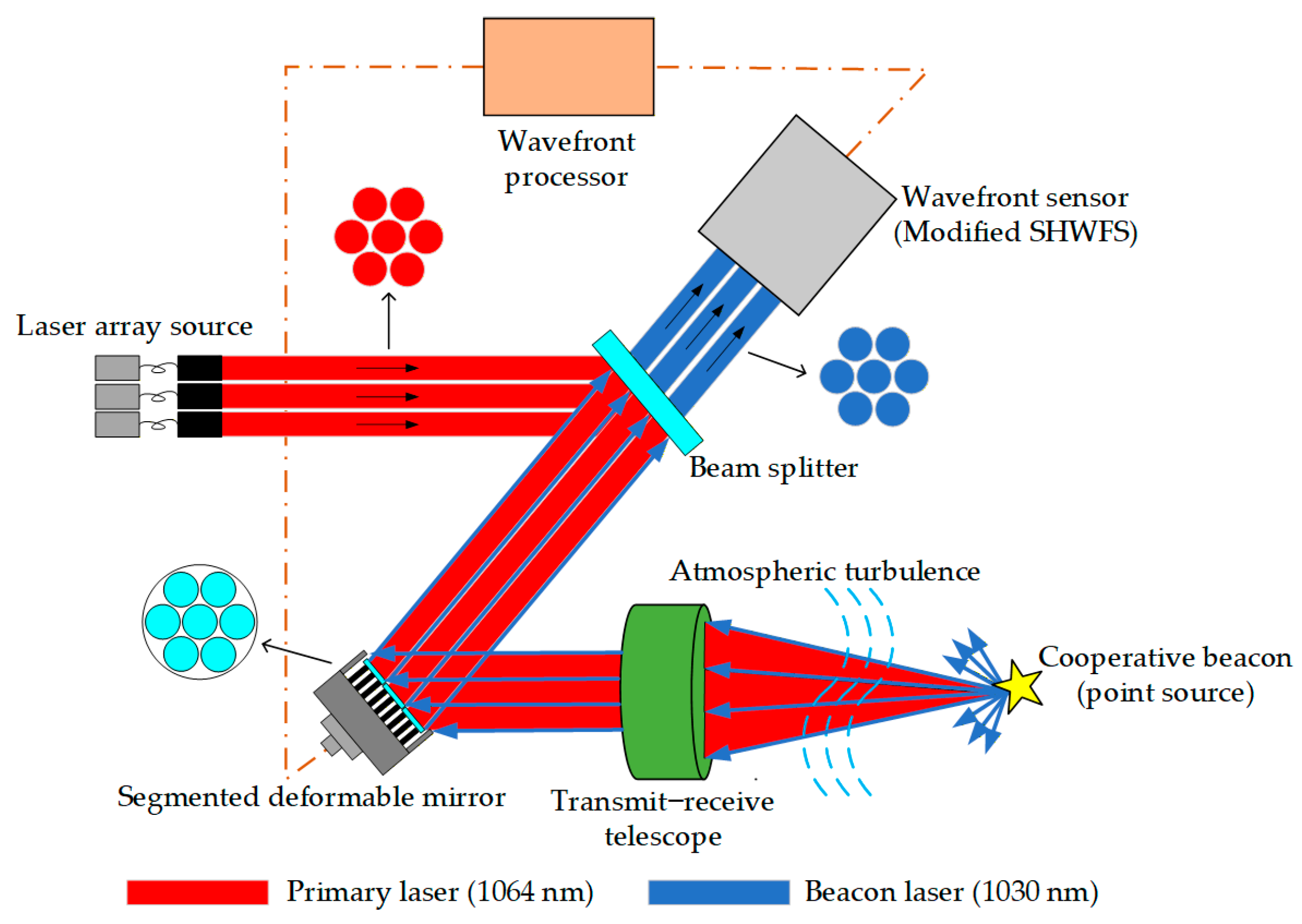
Figure 1 illustrates the schematic diagram of the laser array atmospheric propagation compensation system based on a cooperative beacon. The primary laser array operates at a wavelength of 1064 nm and consists of multiple sub-beams arranged in a regular hexagonal pattern. This wavelength is chosen as a typical near-infrared band that is commonly used in high-power fiber laser systems. The emitted beams are initially collimated and then are sequentially reflected by a beam splitter and an SDM. The SDM is used to compensate the tip–tilt aberration for each sub-beam. In the transmission path, the shared-aperture transmit–receive telescope focuses the laser array onto the distant target through the atmosphere. It is emphasized that the system utilizes a continuous-wave (CW) laser array rather than a pulsed laser.

The cooperative beacon, located at the target, is modeled as a point source at a wavelength of 1030 nm. The beacon light propagates back through the same atmospheric path as the outgoing laser, thereby carrying the turbulence-induced aberrations accumulated along the propagation path. In the reception path, the diffuse beacon light is collected by the telescope and converted into a collimated beam. When it is reflected by the SDM, the continuous wavefront is spatially segmented into multiple discrete portions by the independent sub-mirrors. The segmented wavefronts then match the discrete spatial distribution of the primary laser array.

The 1030 nm beacon light and the 1064 nm primary laser have a small wavelength separation, which ensures that they experience nearly identical phase disturbance in the atmospheric turbulence. Consequently, the wavefront aberration information carried by the beacon light can represent that of the primary laser. Additionally, 1030 nm lies in a low absorption window, which improves the signal to noise ratio for wavefront detection.

The wavelength difference between 1030 nm and 1064 nm enables efficient spectral separation using a beam splitter. The beam splitter is designed with a multi-layer coating that reflects the primary laser at 1064 nm while transmitting the beacon light at 1030 nm.

The modified SHWFS receives the beacon wavefront according to the relative spatial positions of the laser array and measures the spot displacements for each sub-beam. Based on the displacements, the wavefront processor calculates the corresponding tip–tilt compensation and converts it into control voltages that drive the SDM to correct the tip–tilt aberrations induced by atmospheric turbulence.

To simplify the study of beam combining, incoherent combining is adopted for theoretical and simulation analysis. The near-field complex amplitude can be expressed as the superposition of the complex amplitudes of multiple individual sub-beams, as given by Equation (1). Here, $N$ is the number of sub-beams in the laser array. $\left(x_i,y_i\right)$ denotes the center position of the $i$ sub-beam, and $D$ is the effective aperture of the laser array.

$${\tilde{U}}_{\left(x_i,y_i\right)}\left(x,y\right)={\displaystyle \sum _{i=1}^N{A}_i\left(x-x_i,y-y_i\right)}\exp \left[j\phi \left(x-x_i,y-y_i\right)\right]$$

(1)

According to Fourier optics [19], the far-field intensity distribution after propagating a distance L in free space can be approximated by the Fourier transform of the near-field complex amplitude. For incoherent combining, the synthesized far-field intensity is the sum of the far-field intensities of the individual sub-beams, expressed as:

$$I_{far}\left(f_x,f_y\right)={{\displaystyle \sum _{i=1}^N\left\{{\left|FFT\left[{\tilde{U}}_{\left(x_i,y_i\right)}\left(x,y\right)\right]\right|}^2\right\}}}_{|f_x={\displaystyle \frac{x}{\lambda L}},f_y={\displaystyle \frac{y}{\lambda L}}}$$

(2)

2.2. Atmospheric Turbulence Phase Screen Model

The atmospheric turbulence phase screen method is an effective numerical simulation approach for studying the influence of turbulence on laser propagation. Considering that the simulation aperture is circular and that each order of the Zernike polynomials corresponds to specific wavefront aberrations, the Zernike polynomial method is adopted in this paper to generate the atmospheric turbulence phase screen following the Kolmogorov spectrum [20,21,22]. The phase screen wavefront is represented by a series expansion of orthogonal Zernike polynomials, as expressed in Equation (3), where $Z_k\left(x,y\right)$ denotes the $k$ order Zernike polynomial, $a_k$ is its corresponding coefficient, and K is the total number of modes considered.

$$\phi \left(x,y\right)={\displaystyle \sum _{k=1}^K{a}_k\cdot Z_k\left(x,y\right)}$$

(3)

To investigate the effect of the temporal characteristics of atmospheric turbulence, a time-dependent stochastic process is introduced into the Zernike coefficients to generate a time-varying sequence of phase screen [23]. This paper employs the spline interpolation method to generate the sequence of phase screen. The principle of this method is to introduce a time-dependent variable $X_k\left(t\right)$ with specific statistical properties into the static atmospheric turbulence phase screen constructed by using the Zernike polynomial method. For each Zernike mode, a discrete temporal sequence is generated as:

$$b_k(t)=X_k\left(t\right)\cdot a_k$$

(4)

The coefficient $b_k\left(t\right)$ at each time follows a Gaussian random noise with mean zero and variance $〈b_k^2〉$. According to the turbulence phase mean square residual defined by Noll and the empirical relationship of the mean square residual derived by Fried, the time-averaged value of $b_k^2$, i.e., the ensemble average $〈b_k^2〉$, can be recursively obtained. Cubic spline interpolation is then applied to the discrete sequence $b_k\left(t\right)$ to obtain smooth and continuous temporal variations. Subsequently, the phase screen at each time t can be obtains by substituting the coefficient in Equation (3).

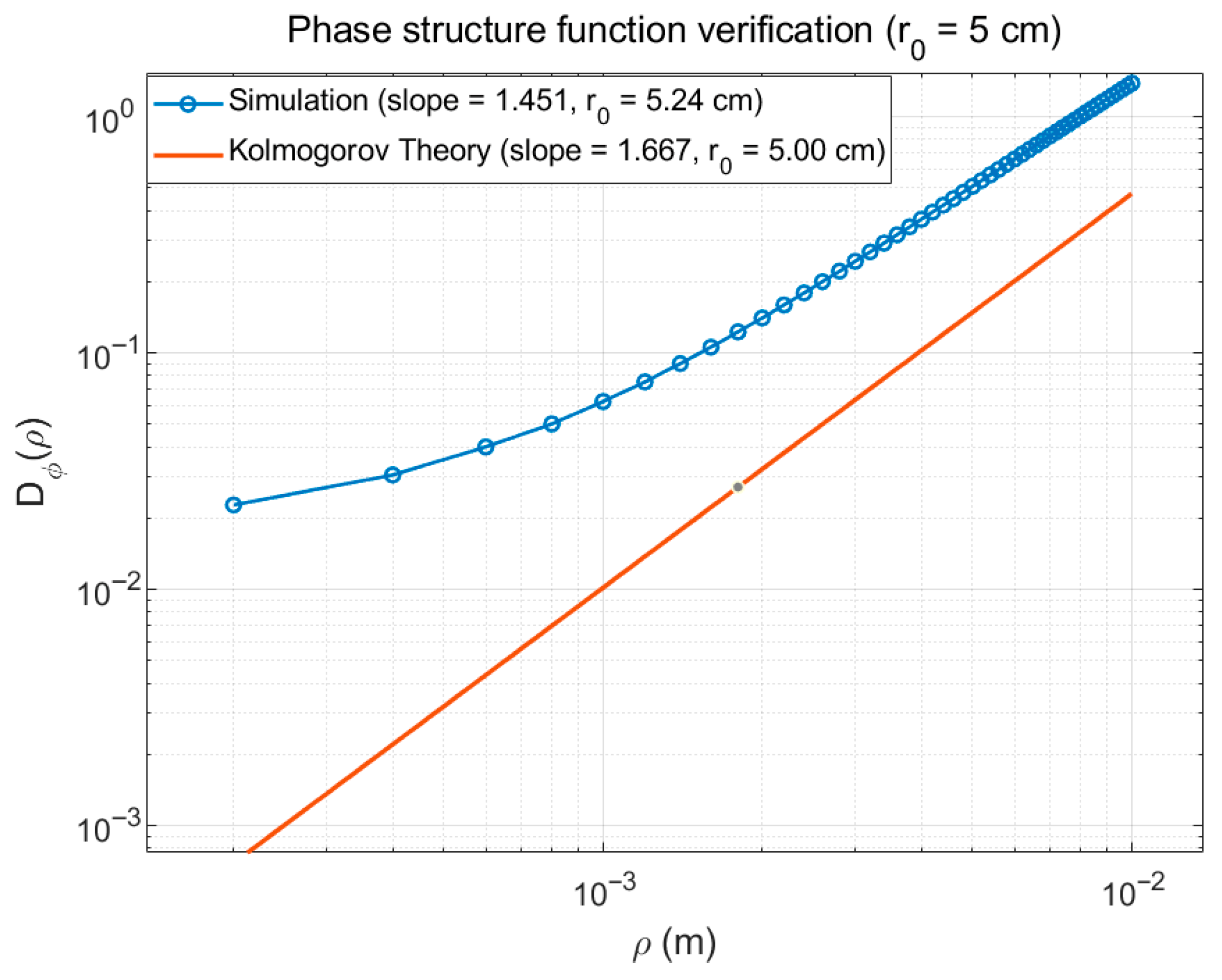
To verify that the generated phase screens satisfy the prescribed turbulence strength, the phase structure function $D_{\mathrm{\varphi }}(\rho )$ is computed and compared with the theoretical prediction of the Kolmogorov model. According to Kolmogorov turbulence theory, the phase structure function is calculated by:

$$D_{\mathrm{\varphi }}(\rho )=\langle {[\mathrm{\varphi }(r)-\mathrm{\varphi }(r+\rho )]}^2\rangle =6.88{\left({\displaystyle \frac{\rho }{r_0}}\right)}^{5/3}$$

(5)

A sequence of 100 phase screens was generated with a preset atmospheric coherence length of $r_0=5\mathrm{cm}$ with 120 Zernike orders. The final numerical structure function ${\overline{D}}_{\mathrm{\varphi }}(\rho )$ is obtained by taking the ensemble average over 100 frames. Furthermore, the estimated coherence length $r_{0,fitted}$ is extracted by fitting ${\overline{D}}_{\mathrm{\varphi }}(\rho )$ to the theoretical Kolmogorov model in Equation (5) using the nonlinear least-squares algorithm. The validation result is illustrated in Figure 2. The numerical structure function obtained from the simulated phase screen sequence follows the power-law trend predicted by Kolmogorov theory. The fitting result yields $r_{0,fitted}=5.24\mathrm{cm}$, which is in close agreement with the preset value ($r_0=5\mathrm{cm}$) with a relative error of only 4.8%.

This minor difference is primarily attributed to the finite number of Zernike orders in the expansion for high-frequency representation and to statistical fluctuations inherent in the ensemble average over a finite sequence of 100 phase screens. The overall statistical consistency confirms that the generated phase screens accurately reproduce the intended turbulence strength.

2.3. Tip–Tilt Aberration Detection of Sub-Beams

In a single-laser AO system, tip–tilt aberration appears as a global phase slope across continuous sub-apertures measured by the SHWFS, resulting in a shift of the far-field spot position. In contrast, a laser array AO system exhibits both a global tip–tilt component and differential tip–tilt components among the sub-beams. These effects result in not only an overall drift of the synthesized far-field spot but also splitting and broadening. The discrete and multi-variate nature of the tip–tilt aberration in laser array requires a dedicated sensing scheme that measures the tip–tilt of each sub-beam separately. Therefore, this study employs a modified SHWFS with discrete sub-apertures matched to the spatial layout of the sub-beams, which ensures the independent measure for each channel.

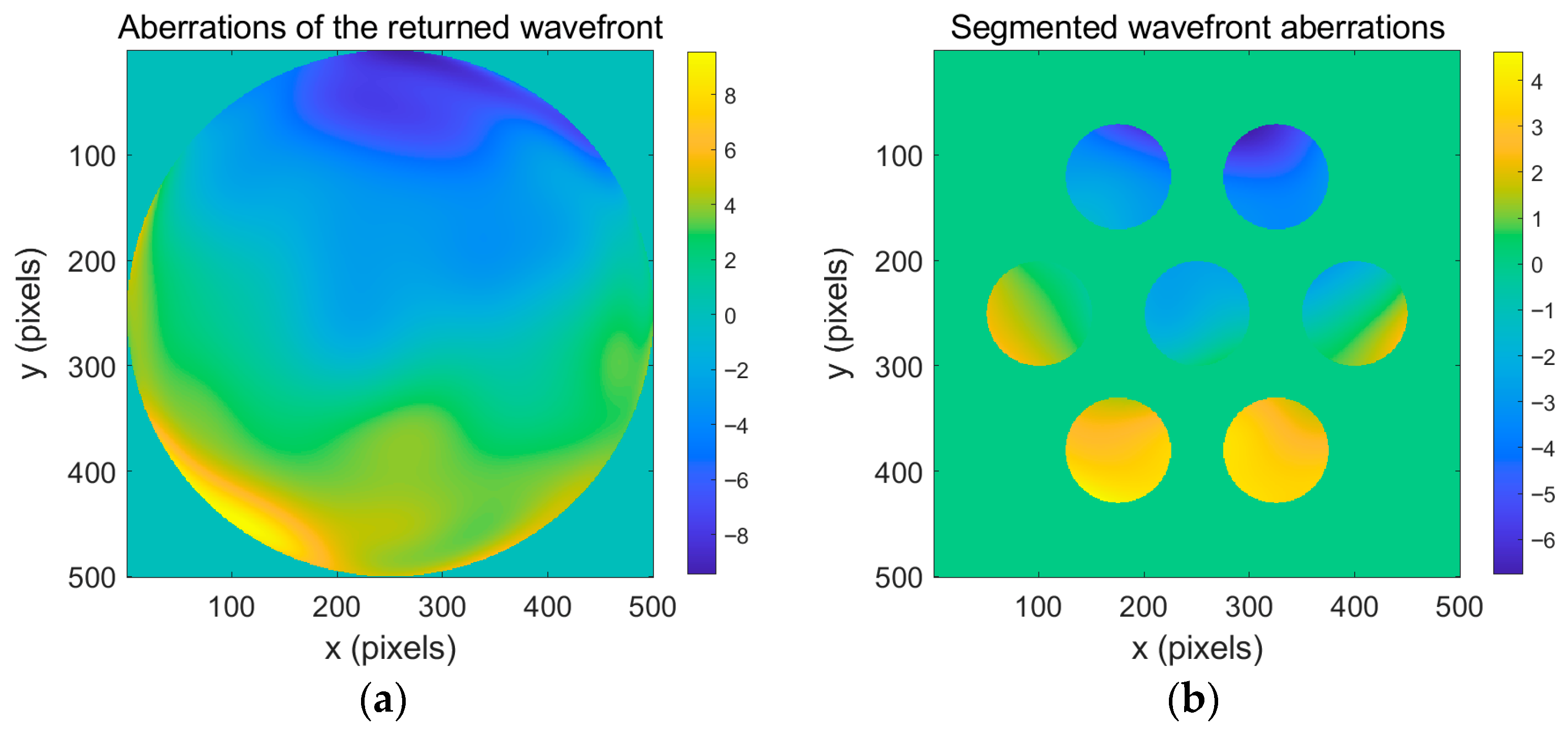
As described in the model of the system in Section 2.1, the modified SHWFS detects the tip–tilt aberration introduced by atmospheric turbulence along the laser propagation path using the light from the cooperative beacon. The returned wavefront is segmented according to the relative spatial arrangement of the sub-beams, as shown in Figure 3.

Distinct from a traditional SHWFS, which spatially samples a continuous pupil into multiple sub-apertures to measure local gradients, the modified SHWFS is specifically configured for the discrete aperture distribution of the laser array. The number of sub-apertures in the microlens array is equal to the number of sub-beams, and a one-to-one correspondence is established between each sub-aperture and its associated sub-beam. Each sub-beam is focused by its corresponding microlens onto the CCD sensor, forming an individual focal spot.

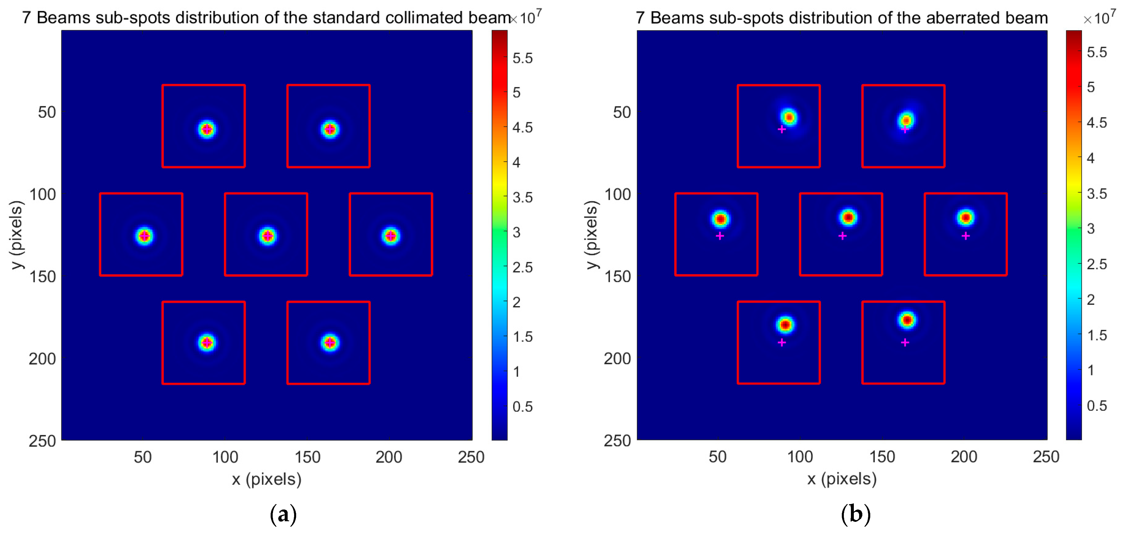
The operating principle of the modified SHWFS is similar to that of a conventional SHWFS. During calibration, a standard collimated laser array is used to determine the reference centroid positions of all sub-spots. When the returned beam affected by atmospheric turbulence is incident, each sub-spot is displaced relative to its reference position, as shown in Figure 4. The centroid displacement in the x/y direction of each sub-spot can be calculated using a centroid algorithm:

$$\left\{\begin{array}{l}{x}_c={\displaystyle \frac{{\displaystyle \sum _i{\displaystyle \sum _j{x}_{i,j}}}\cdot I(x_{i,j},y_{i,j})}{{\displaystyle \sum _i{\displaystyle \sum _{j}I}}(x_{i,j},y_{i,j})}}\hfill \\ y_c={\displaystyle \frac{{\displaystyle \sum _i{\displaystyle \sum _j{y}_{i,j}}}\cdot I(x_{i,j},y_{i,j})}{{\displaystyle \sum _i{\displaystyle \sum _{j}I}}(x_{i,j},y_{i,j})}}\hfill \end{array}\right.$$

(6)

Since the modified SHWFS measures the displacement of each sub-beam with respect to a global reference coordinate frame, the feedback control loop simultaneously compensates both the global tip–tilt component and the local tip–tilt components of individual sub-beams. This approach eliminates the need for an additional global tip–tilt mirror and simplifies the system architecture while maintaining accurate sensing and correction.

2.4. Tip–Tilt Aberration Compensation of Sub-Beams

Closed-loop control is implemented using the direct slope method and the proportional–integral (PI) algorithm. The wavefront corrector is an SDM composed of multiple independent sub-mirrors, each corresponding to one sub-beam. Each sub-mirror is rigid and driven by three actuators arranged in an equilateral triangle configuration, enabling piston motion or tip–tilt in the x/y direction. Since each sub-mirror requires two degrees of freedom (tip and tilt) for correction, the control system involves $2N$ driving channels for an array of $N$ sub-beams.

Before closed-loop control, the interaction matrix $T$ between the actuator voltages of the SDM and the spot centroid displacement of the modified SHWFS must be experimentally determined. Let the control voltage vector applied to the actuators be $V={[v_1,v_2,\dots ,v_{2N}]}^T$ and the corresponding centroid displacement vector be $D={[\mathrm{\Delta }{x}_1,\mathrm{\Delta }{y}_1,\dots ,\mathrm{\Delta }{x}_N,\mathrm{\Delta }{y}_N]}^T$. Under the assumption of a linear system response, their relationship is expressed as:

$$D=T\cdot V$$

(7)

where $T\in {ℝ}^{2N\times 2N}$ is the interaction matrix, which is experimentally determined by sequentially applying unit voltages to the two actuators of each sub-mirror and recording the resulting centroid shifts in all sub-apertures. The element $T_{ij}$ presents the response of the $i$ sensor coordinate to the $j$ actuator.

The control matrix is obtained by calculating the Moore-Penrose pseudo-inverse of $T$, denoted as $T^{+}$. Based on the real-time measurement of the centroid displacement vector $D_t$, the required correction voltage vector $V_t$ is calculated by:

$$V_t=T^{+}\cdot D_t$$

(8)

A PI algorithm is adopted for closed-loop control, and the iterative process is given by:

$$V_{t+1}=K_p\cdot V_{error}+K_i\cdot V_{integral}$$

(9)

$$V_{integral}=V_{integral}+V_{error}$$

(10)

where $V_{t+1}$ is the updated actuator voltage vector used for correction. $V_{intergral}$ is the integral term initialized as a zero vector. $K_p$ represents the proportional gain and $K_i$ represents the integral gain.

During each iteration, the updated actuator voltages drive the SDM to generate the required tip–tilt compensation, and the modified SHWFS then measures the residual wavefront after compensation. This process is continuously iterated until the convergence condition is satisfied.

3. Simulation Analysis

3.1. Simulation of Tip–Tilt Aberration Compensation

The numerical simulations were performed using MATLAB R2024b. In the numerical simulation, the cooperative beacon light is defined as a circular flat-top laser with a wavelength of 1030 nm while the primary laser array has a wavelength of 1064 nm. The sub-beams are arranged in a regular hexagon with a diameter of 20 mm each and a center-to-center spacing of 30 mm. By varying the number of arrangement ring n (n = 2,3,4…), the corresponding number of sub-beams is given by:

$$N=3n\left(n-1\right)+1$$

(11)

The equivalent aperture of the array beam is adjusted accordingly. The atmospheric coherence length $r_0$ is 5 cm, and the average transverse wind speed $v$ is 3 m/s.

The laser propagation distance is set to 3 km. The total evolution duration of the simulation is 1 s, which corresponds to the total number of frames within the numerical sequence. To characterize the temporal dynamics of atmospheric turbulence, the Greenwood frequency $f_G$ is calculated:

$$f_G={\left[0.102\left({\displaystyle \frac{k^2}{L}}\right){\displaystyle {\int }_0^L{C}_n^2}(z)v^{5/3}(z)dz\right]}^{3/5}\approx 0.43{\displaystyle \frac{v}{r_0}}$$

(12)

Based on the specified parameters, the Greenwood frequency $f_G$ is approximately 25.8 Hz. In the simulation, the frequency of the closed-loop control is set to be significantly higher than $f_G$. Taking a seven-beam laser array as an example, the total simulation duration is 1 s with approximately 250 frames, corresponding to a simulation frequency of about 250 Hz, which is approximately 10 times the $f_G$. Additionally, the time-varying sequence of phase screens is generated by the method of cubic spline interpolation, which ensures that the temporal evolution of the turbulence remains smooth and continuous.

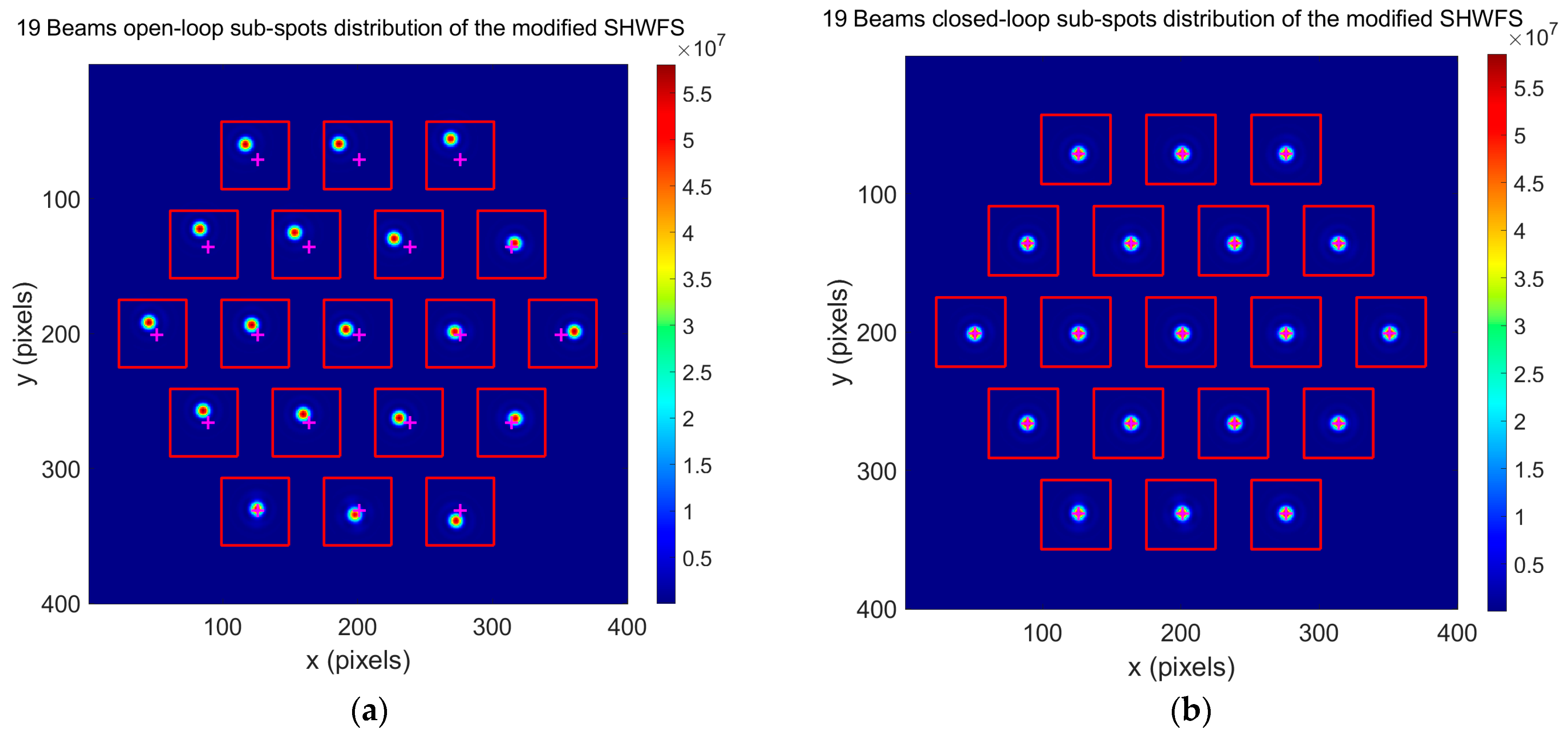
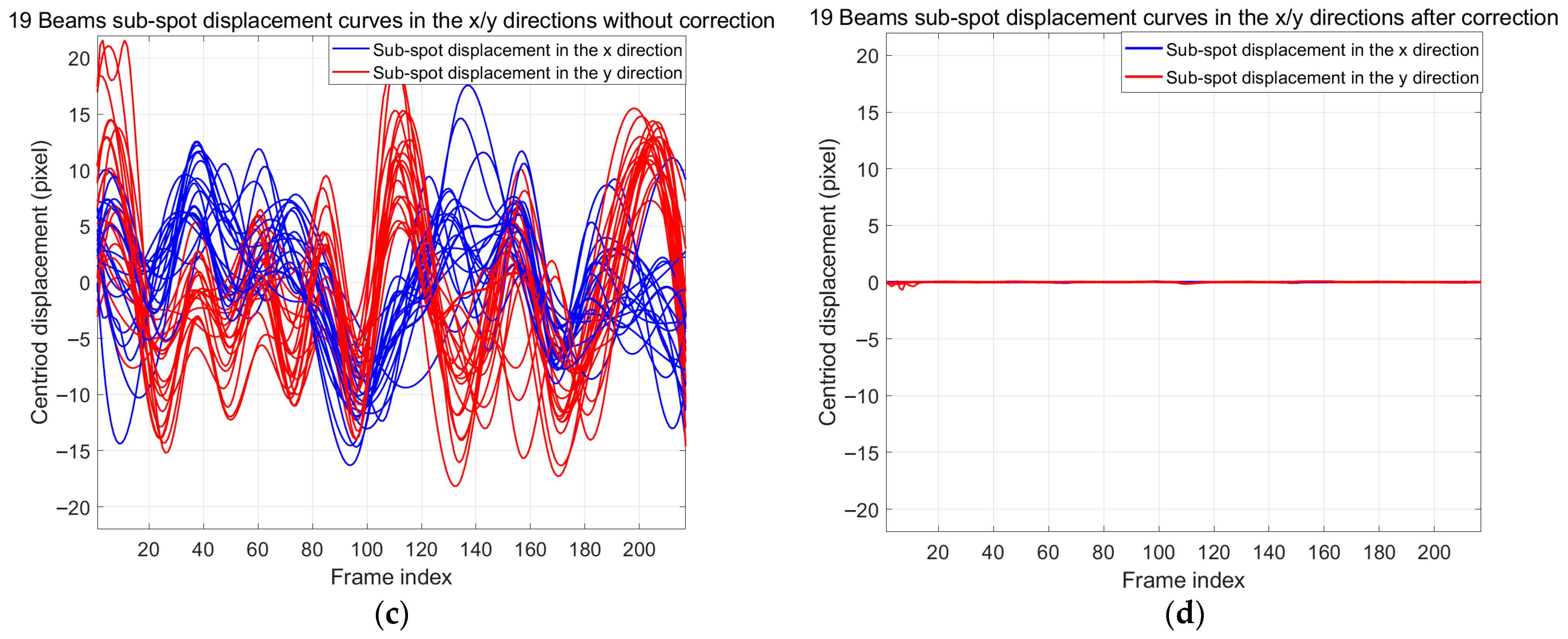
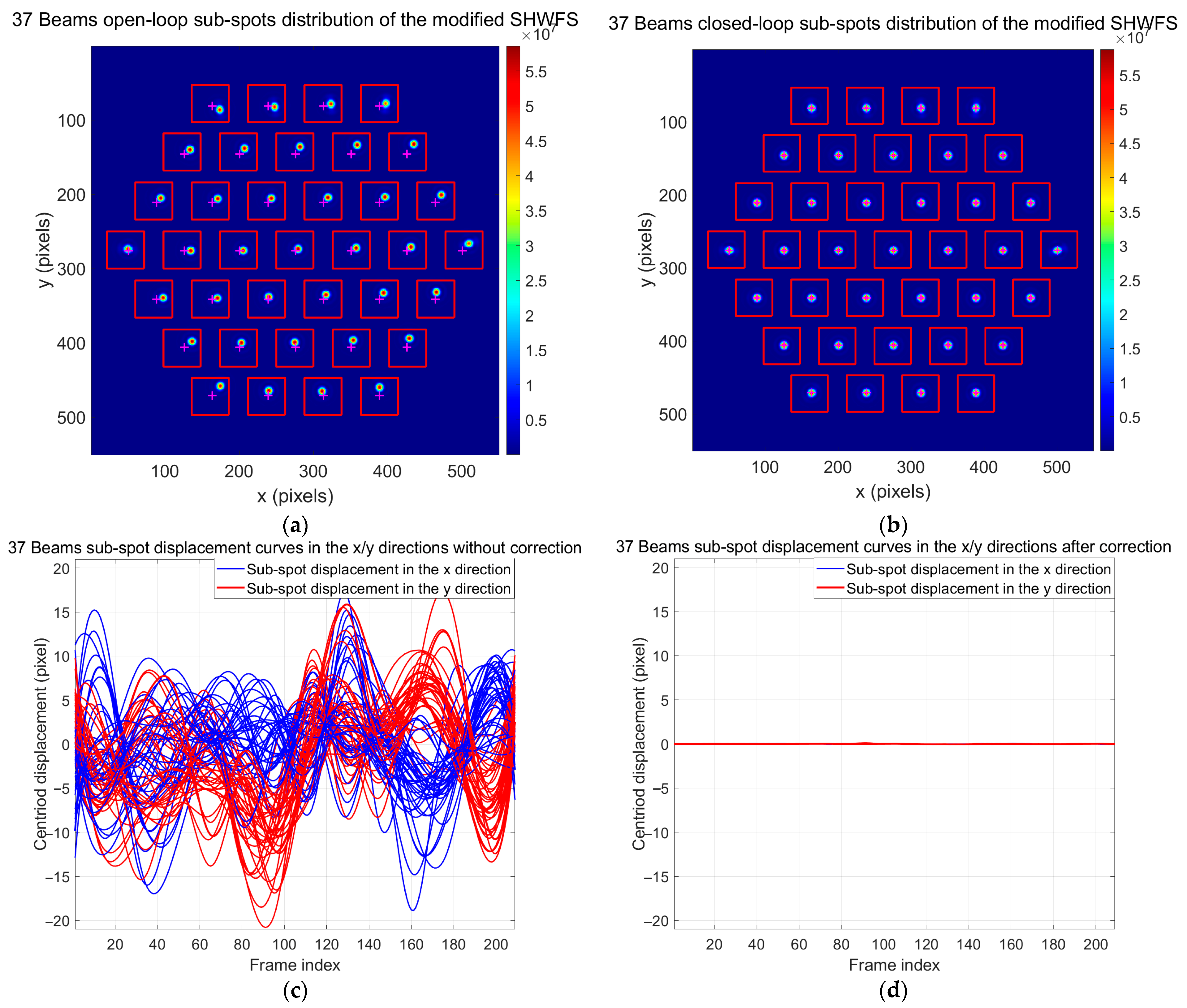
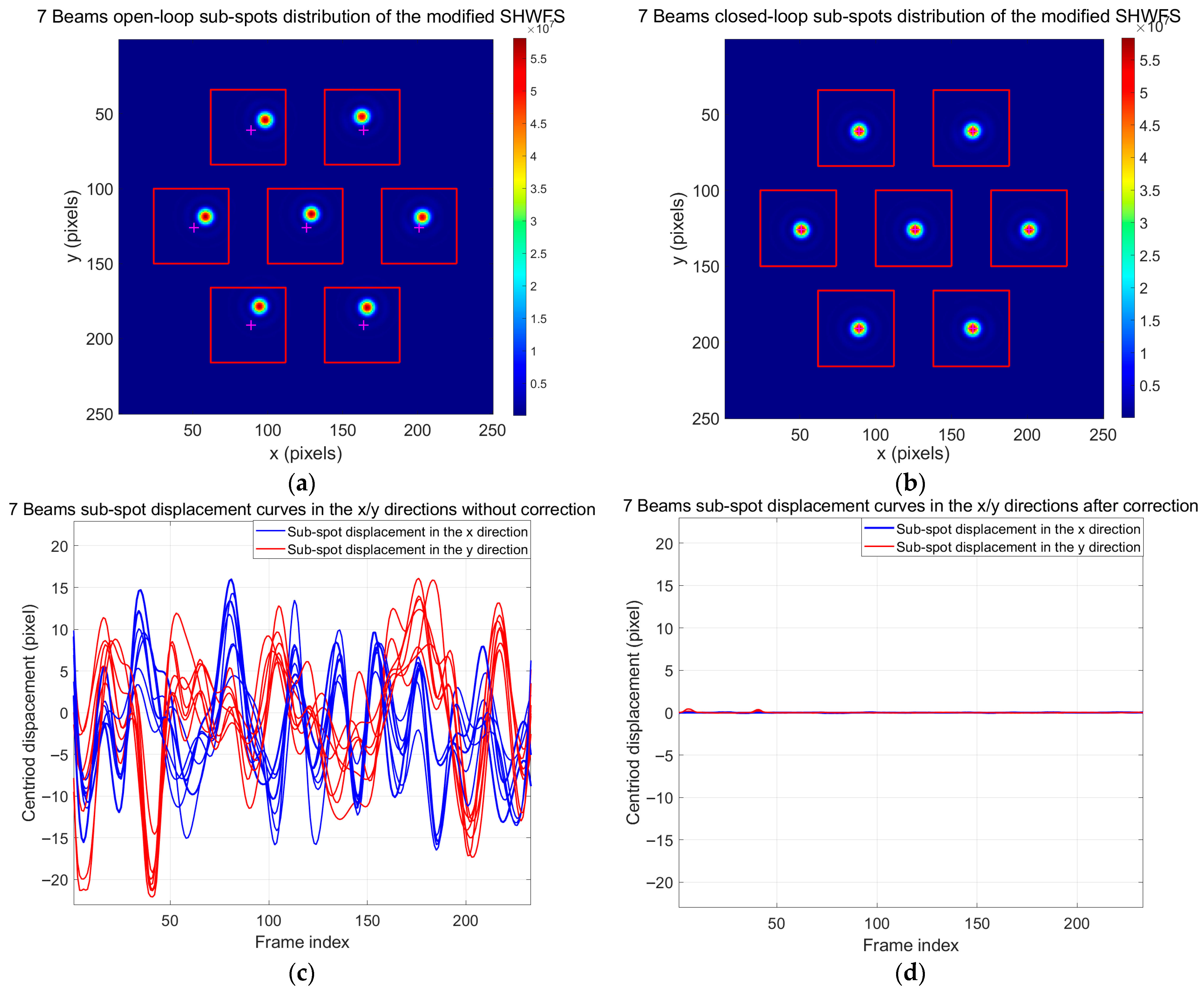
The simulations are conducted for n = 2, 3, and 4 (corresponding to N = 7, 19, and 37). The system performs frame-by-frame detection and correction of the phase screen sequence. Figure 5, Figure 6, and Figure 7 illustrate the sub-spot distributions and centroid displacement curves before and after tip–tilt compensation for n = 2, 3, and 4, respectively. In the open-loop state, the focal sub-spots produced by the modified SHWFS exhibit significant random deviations from their calibrated reference centers (marked by magenta “+” symbols) as a direct consequence of stochastic phase distortions induced by the atmospheric turbulence. It can be observed that the corresponding displacement curves in the x and y directions exhibit high amplitude fluctuations over the 1 s duration, reflecting the dynamic impact of the time-varying phase screens on each sub-beam.

Upon implementation of closed-loop compensation using the proposed system, the tip–tilt aberrations of each sub-beam are effectively suppressed. The sub-spots are driven back to and stabilized at the calibrated zero positions with high precision. The displacement curves after correction remain close to zero with minimal residual jitter, which demonstrates that the control frequency of the system is sufficient to track atmospheric turbulence at this Greenwood frequency. Moreover, the consistent correction performance across the 7-beam, 19-beam, and 37-beam configurations indicates that the system maintains high stability and robust scalability as the complexity of the laser array increases.

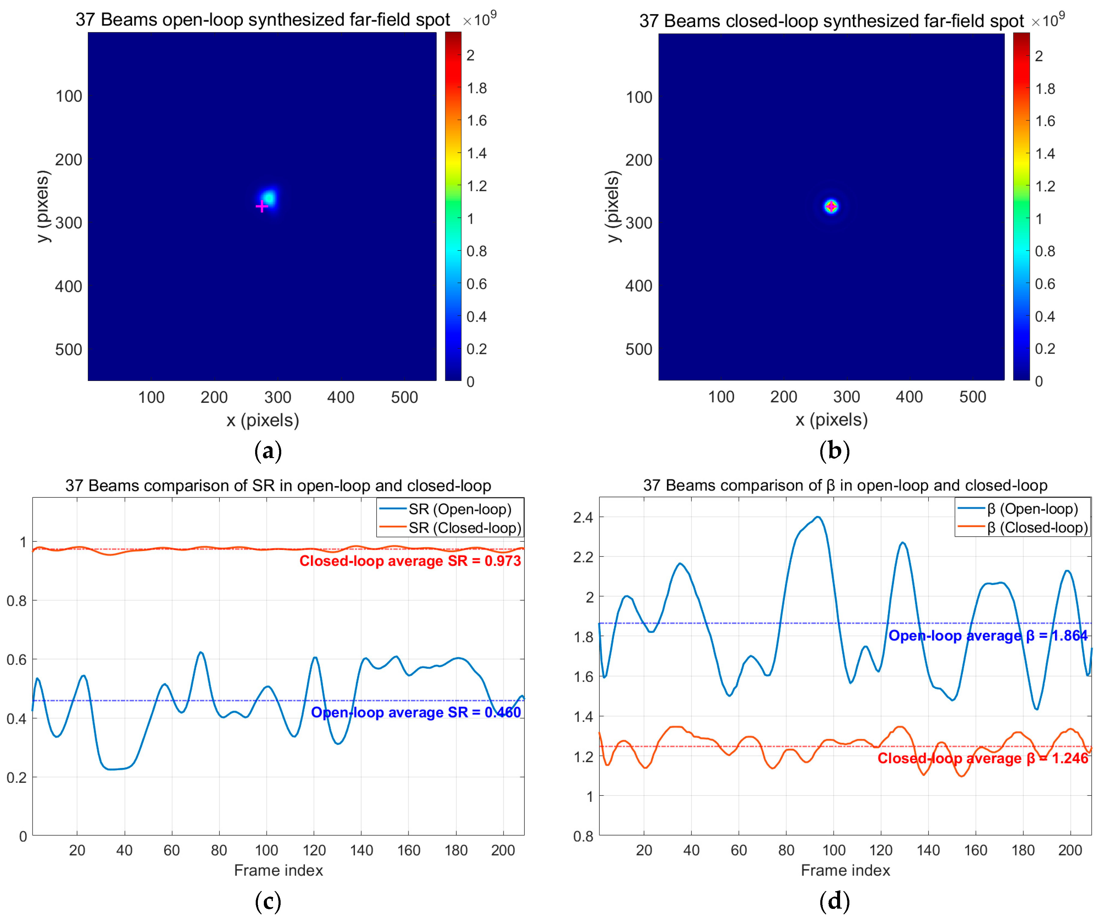
The Strehl ratio (SR) and the beam quality factor β are used as evaluation metrics for far-field beam quality and energy concentration. Specifically, the SR is defined as the ratio of the peak far-field intensity of the aberrated beam to that of the reference beam. A larger SR value (with a maximum of one) indicates better beam quality. The factor β is defined as the ratio of the bucket radius of the aberrated beam to that of the reference beam under a specified power-in-the-bucket threshold in the far-field spot. A smaller β value (with a minimum of one) corresponds to better beam quality and higher concentration of energy.

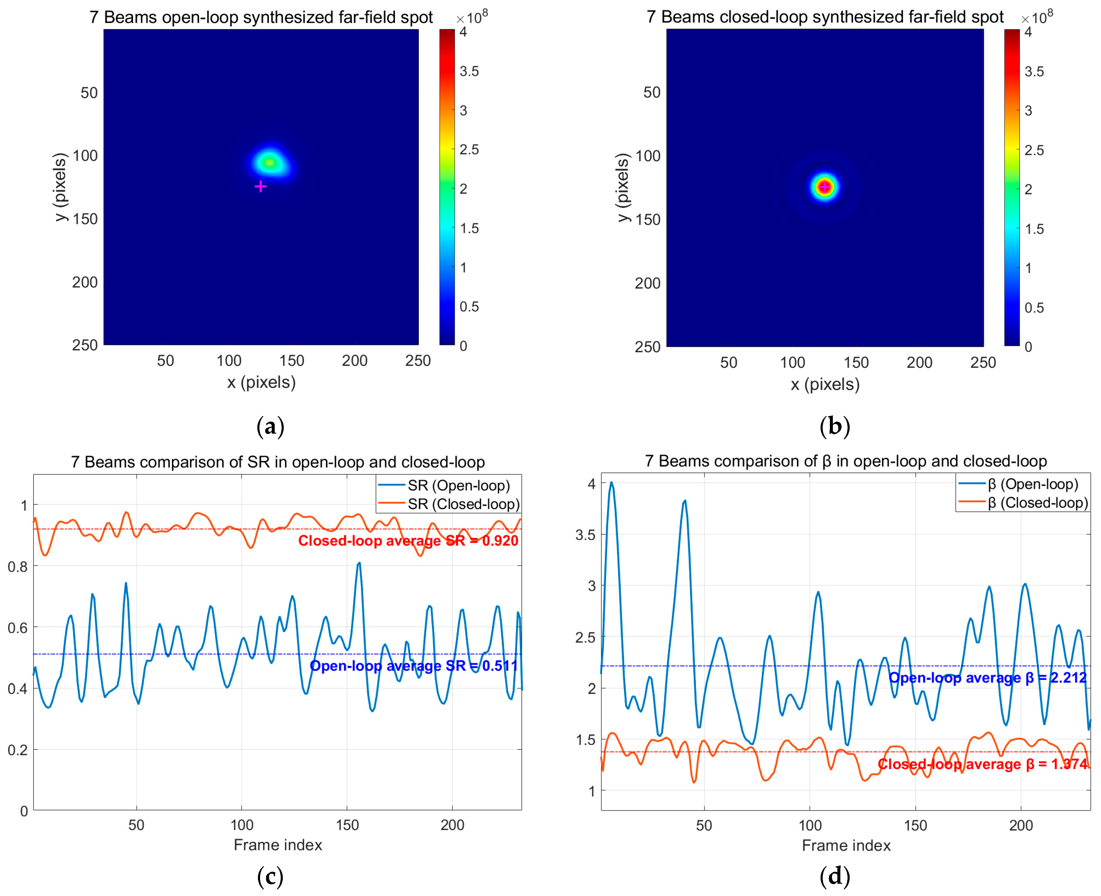
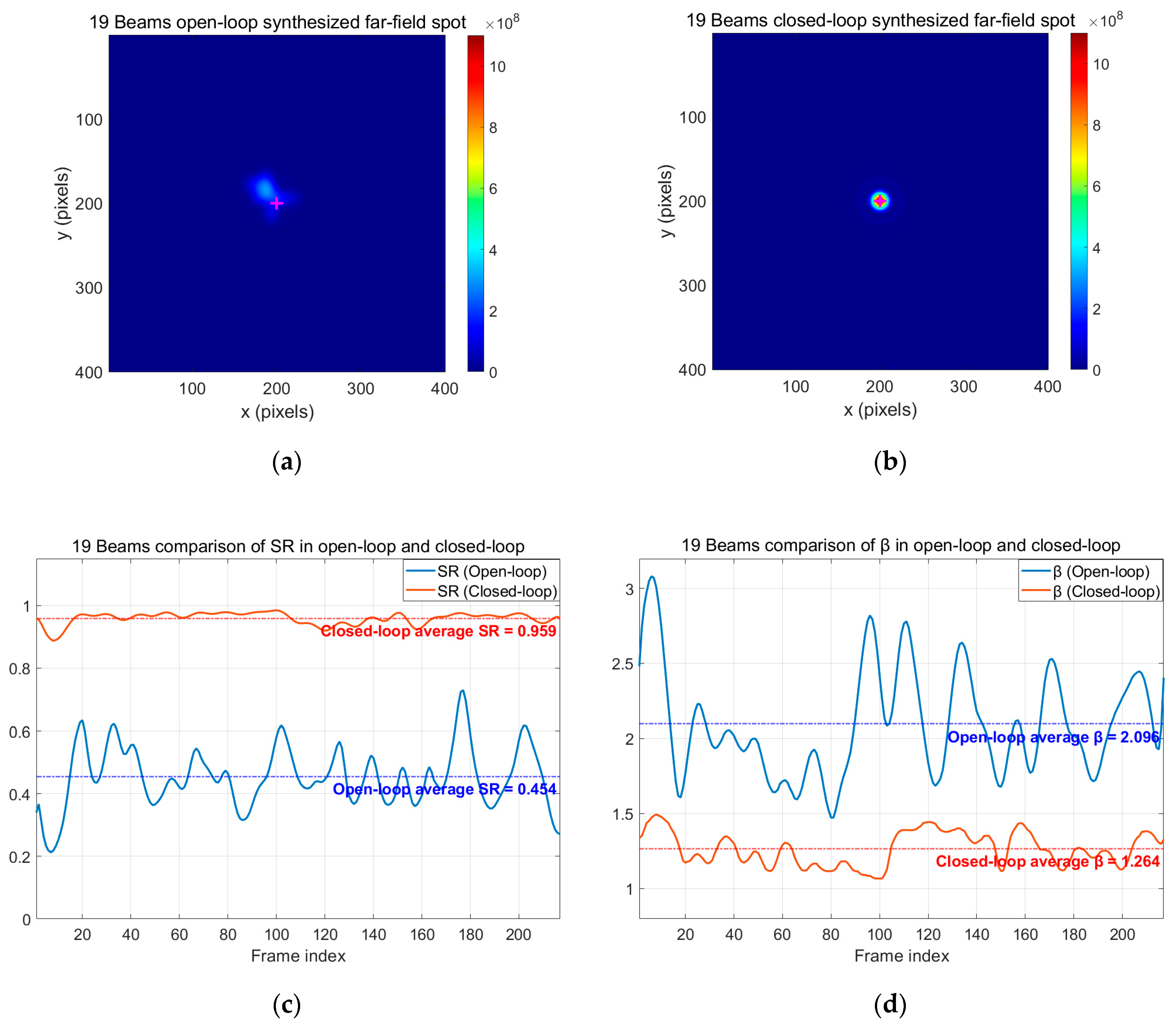
Figure 8, Figure 9, and Figure 10 illustrate the simulation results of comprehensive comparisons of the synthesized far-field spot patterns, as well as the temporal evolution of SR and β curves for n = 2, 3, and 4 (i.e., N = 7, 19, and 37), respectively.

Prior to compensation, the synthesized far-field spots deviate from the reference positions (marked by magenta “+” symbols) and exhibit significant blurring. Meanwhile, their peak intensities are severely reduced. This degradation is primarily attributed to the collective impact of the global tip–tilt and the local difference tip–tilt within the laser array. Upon activation of the closed-loop correction, spot pattern and peak intensity of the synthesized far-field spots are substantially restored. The far-field energy distribution is effectively concentrated into a near-diffraction-limited central lobe.

The SR and β values of all frames in the simulation are calculated and recorded to obtain the average value before and after correction. The average SR and β for the 7-beam, 19-beam, and 37-beam laser array, along with their corresponding improvement factors, are listed in

Table 1. The average SR for the 7-beam, 19-beam, and 37-beam laser array in the simulation.

Sub-Beams	SR (Without Correction)	SR (After Correction)	Improvement Factor of SR
7	0.511	0.920	0.800
19	0.454	0.959	1.112
37	0.460	0.973	1.115

and

Table 2. The average β for the 7-beam, 19-beam, and 37-beam laser array in the simulation.

Sub-Beams	β (Without Correction)	β (After Correction)	Improvement Factor of β
7	2.212	1.374	0.610
19	2.096	1.264	0.658
37	1.864	1.246	0.496

, respectively.

It can be observed that after closed-loop tip–tilt aberration compensation by the proposed system, both the SR and β values of the far-field laser array are significantly improved, leading to enhanced on-target performance of the laser array. Moreover, effective compensation performance of this system is achieved with different numbers of sub-beams (7, 19, and 37). The stability of these metrics across varying numbers of sub-beams further confirms the robust scalability and high correction precision of the proposed laser array compensation scheme.

3.2. Influence of Atmospheric Coherence Length on Compensation Performance

The atmospheric coherence length $r_0$ is a fundamental parameter characterizing the severity of wavefront distortion induced by atmospheric turbulence. A decrease in the value of $r_0$ signifies an increase in the strength of the turbulence, which leads to more pronounced wavefront aberrations. 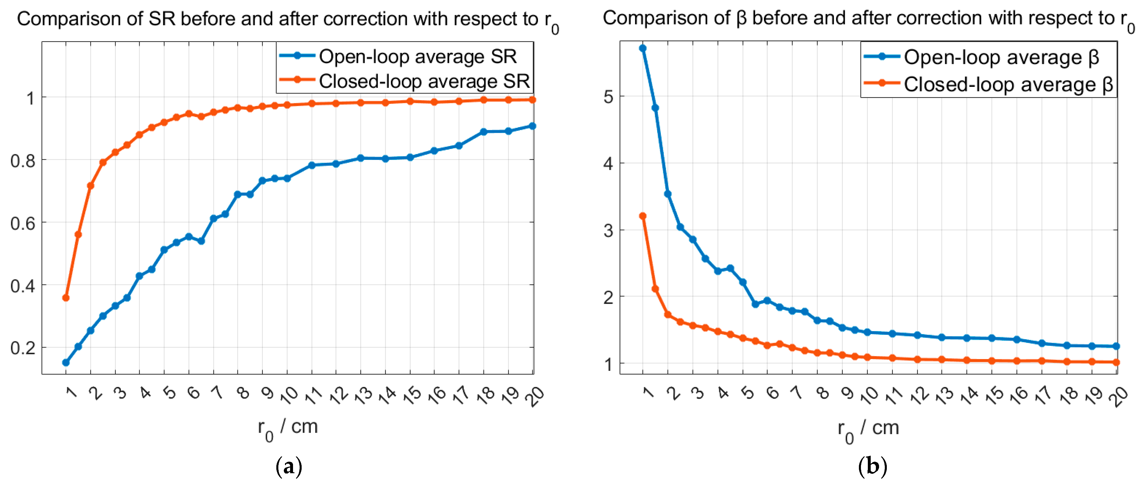To evaluate the robustness of the proposed correction system across varying turbulence conditions, numerical simulations were conducted with $r_0$ ranging from 1 cm to 20 cm with a step size of 1 cm (10~20 cm) and step size of 0.5 cm (1~10 cm). For a seven-beam laser array, the average SR and β curves as functions of $r_0$ are shown in Figure 11, maintaining a propagation distance of 3 km and a transverse wind speed of 3 m/s.

The numerical results in Figure 11 demonstrate the high correction efficiency and robust environmental adaptability of the proposed system. As $r_0$ decreases from 20 cm to 2 cm, the open-loop average SR decreases significantly from 0.91 to 0.25, and the open-loop average β increases from 1.25 to 5.72. Nevertheless, the closed-loop correction system maintains average SR above 0.72 and average β below 1.72, demonstrating consistent compensation capability of the system even as the turbulence strength increases by an order of magnitude. It is worth noting that when $r_0$ ranges from 8 cm to 20 cm, the average SR after closed-loop correction remains above 0.97, while the average β stays below 1.12. This indicates that under weak-to-moderate turbulence conditions, the system approaches the diffraction limit.

When $r_0$ lies in the range from 1 cm to 2 cm, an extremely steep variation in closed-loop performance is observed. Although the open-loop beam quality is severely degraded under this extreme condition, the closed-loop system still increases the average SR from 0.15 to 0.36 and reduces the average β from 5.72 to 3.21, corresponding to a performance gain of approximately a factor of two. This performance limitation at $r_0<2\mathrm{cm}$ is primarily determined by the dynamic range of the modified SHWFS. When the tip–tilt induced by the strong turbulence exceeds the field of view of a sub-aperture, centroid clipping and spot crossover occur, which introduces nonlinear sensing errors.

4. Principle Validation Experiment

4.1. Experimental System and Configuration

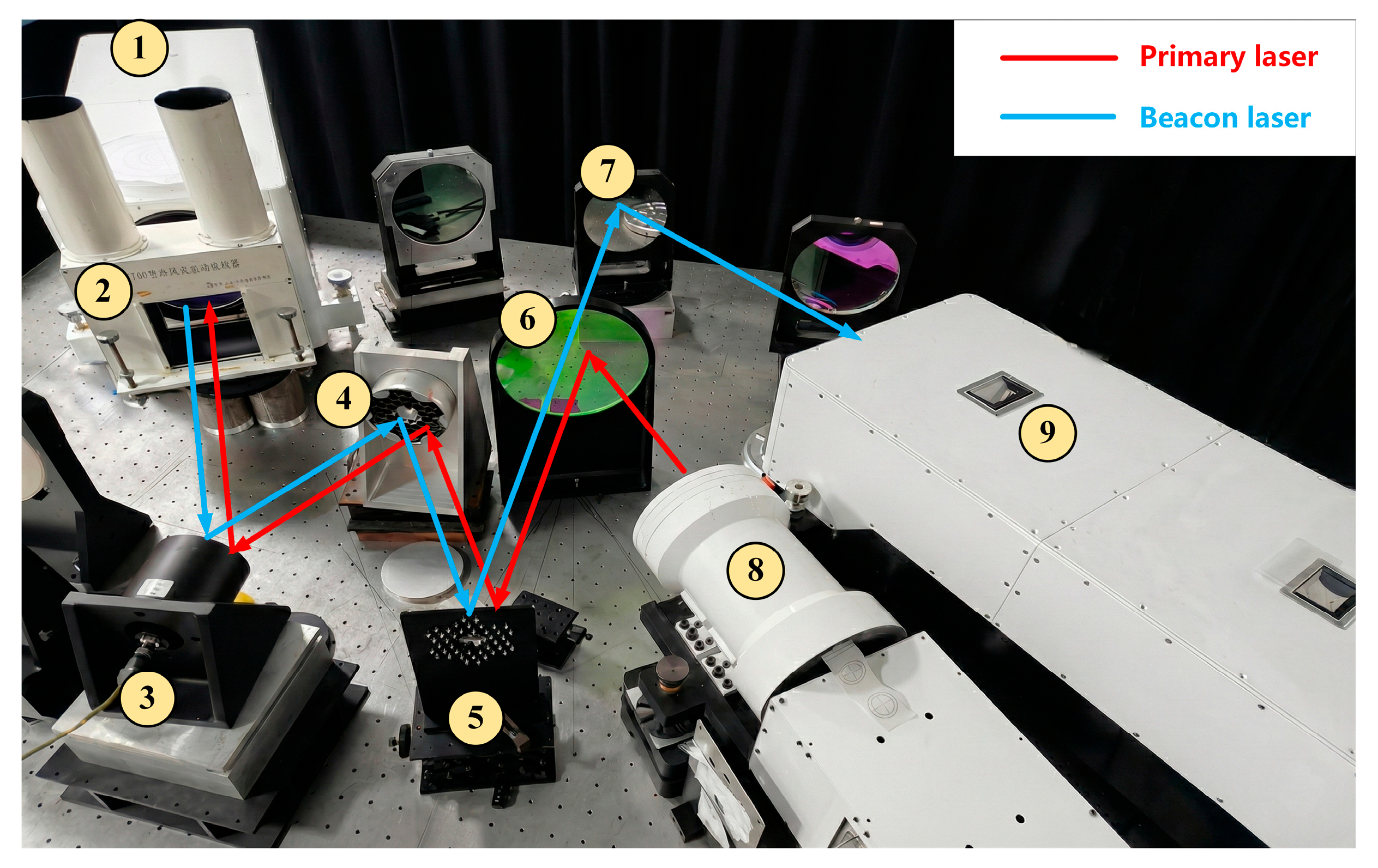
Based on the verification optical path, the constructed experimental setup is shown in Figure 12. The experiment is intended as a principle validation rather than a full-scale atmospheric propagation test, and therefore a turbulence simulator is employed. The experimental system utilizes a 30-beam laser array (self-developed by Institute of Optics and Electronics, Chinese Academy of Sciences, Chengdu, China) with an output wavelength of 1064 nm and a beacon with wavelength of 1030 nm. The sub-beams of the laser array have an aperture of 16 mm and a center-to-center spacing (pitch) of 17 mm.

The laser emitted from the primary laser source sequentially passes through a beam splitter, an array mirror, an SDM (self-developed by Institute of Optics and Electronics, Chinese Academy of Sciences, Chengdu, China), a disturbance tip–tilt mirror, and a turbulence simulator before entering the cooperative beacon. The atmospheric coherence length $r_0$ of the turbulence simulator is approximately 2 cm, which is chosen to verify effective compensation performance of the proposed system under the severe environment. A far-field imaging detector is integrated in the cooperative beacon to measure the beam quality of the outgoing laser. The beacon light then propagates backward along the same optical path and is directed to the wavefront sensor (Modified SHWFS, self-developed by Institute of Optics and Electronics, Chinese Academy of Sciences, Chengdu, China), where the turbulence-induced aberrations along the transmit path are measured. The CCD camera integrated within the modified SHWFS is a short-wave infrared camera, C-RED 2 (First Light Imaging, Meylan, France).

The detailed specifications of the experimental components and parameters are summarized in

Table 3. Detailed specifications of the experimental system components.

Component	Parameter	Value
Primary Laser Array	Number of sub-beams	30
	Wavelength	1064 nm
	Sub-beam aperture	16 mm
	Beam pitch (center-to-center)	17 mm
	Power per sub-beam	20 mW
Cooperative Beacon	Wavelength	1030 nm
	Power	30 mW
Modified SHWFS	Number of microlenses	30
	Image resolution	512 × 512 pixels
	Pixel size	8 μm
	Frame rate	1000 Hz
SDM	Material	Piezoelectric ceramics
	Segment size	16 mm
	Degrees of freedom	3 per segment

.

4.2. Experimental Results and Discussion

It should be noted that a central obscuration is inevitably introduced into the primary laser array and beacon wavefront because the experimental system uses a reflective beam-reduction subsystem. Therefore, sub-spot images of the modified SHWFS contain a centrally blocked region, and the SDM is modified accordingly. The 30-beam laser array in the experiment corresponds to the 37-beam configuration (i.e., n = 3) in the simulation, except that the central 7 sub-beams are blocked. In contrast, the numerical simulation is conducted under an ideal aperture without this central obscuration. This simulation setting is adopted to better investigate the scalability and stability of the proposed method as the size of laser array increases (e.g., n = 2, 3, 4…).

Although the central obscuration reduces the effective aperture and changes the far-field energy distribution, which in turn biases the absolute values of SR and β, this effect does not diminish the validity of the proposed method. Since the central obscuration remains unchanged throughout the experiment, its influence is consistent in both open-loop and closed-loop cases. The evaluation of this study focuses on the relative improvement from open-loop to closed-loop. Consequently, the improvement trends of SR and β remain reliable indicators of the correction system performance.

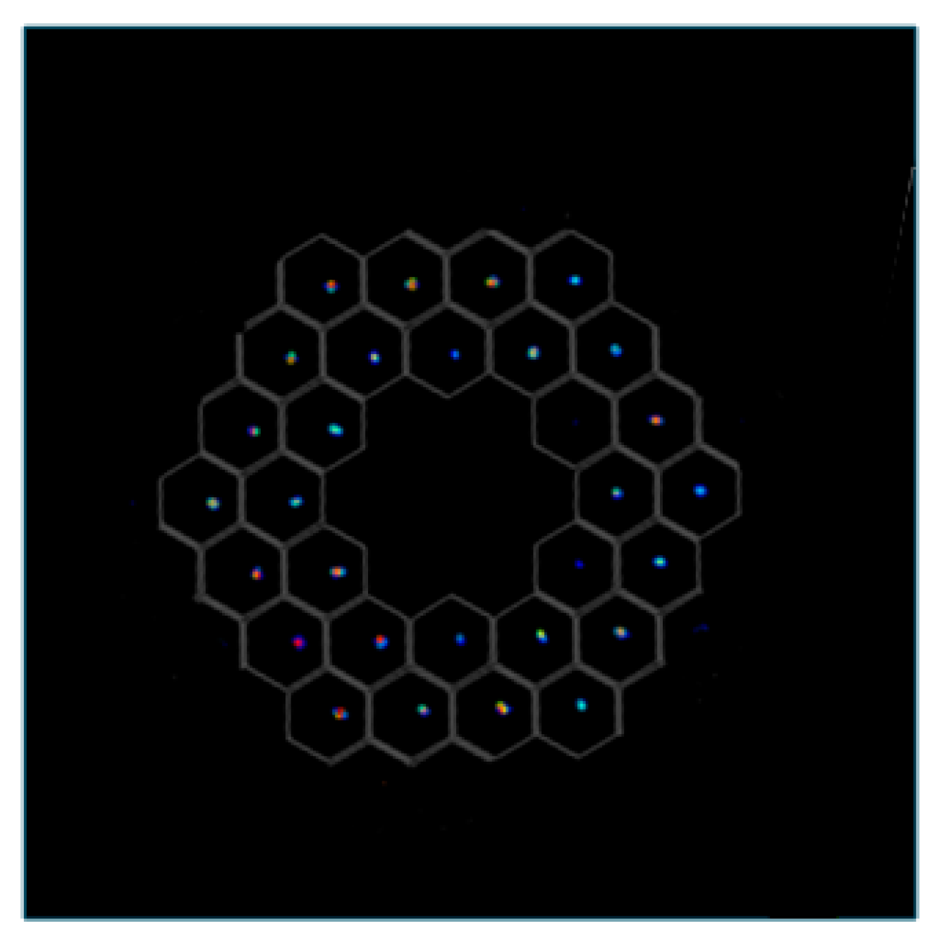
Under the condition of an atmospheric coherence length $r_0$ of 2 cm, the sub-spots image of the beacon light obtained by the modified SHWFS is shown in Figure 13. Each single sub-beam enters its corresponding sub-aperture, enabling real-time measurement of the tip–tilt for each sub-beam.

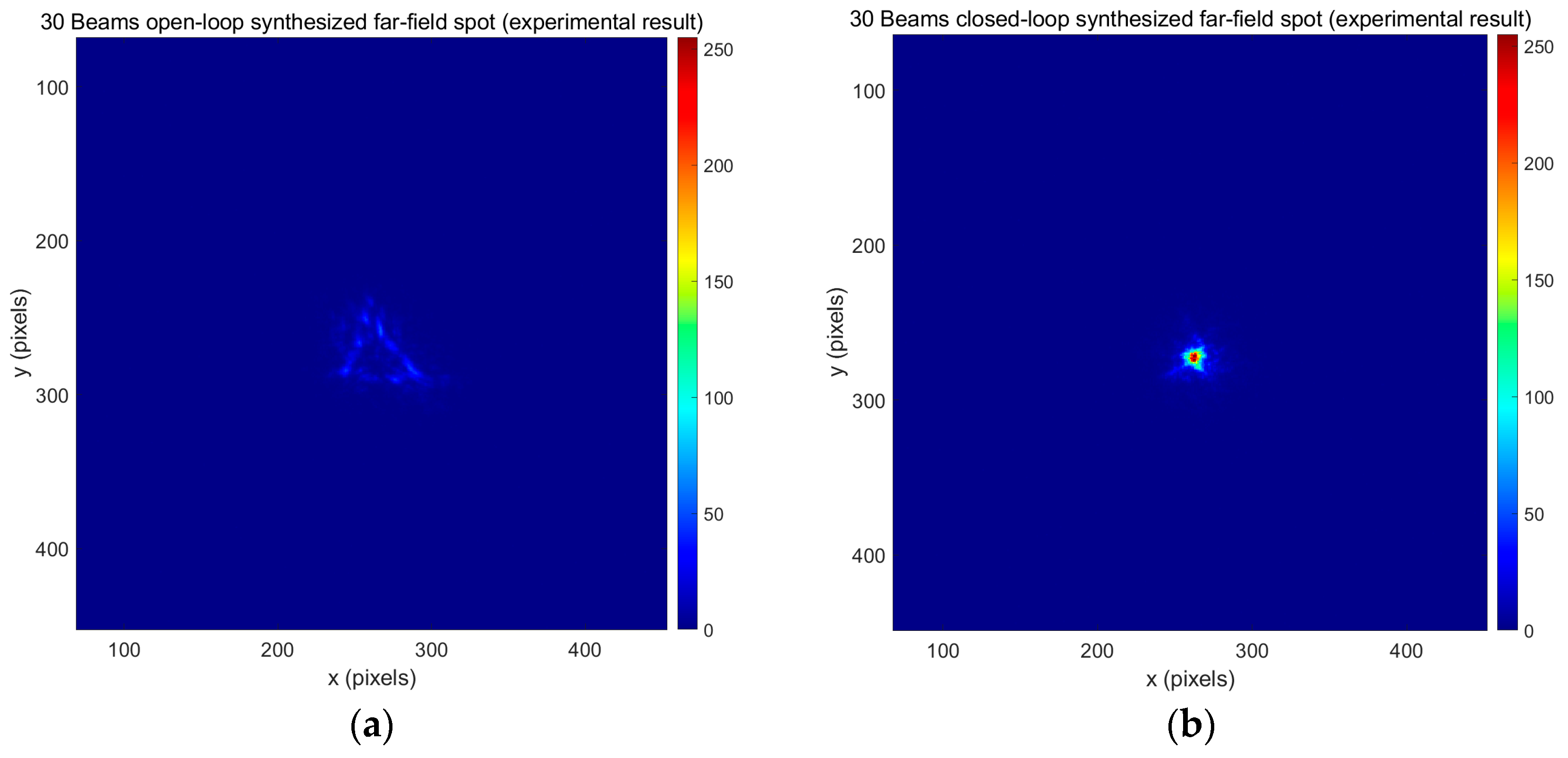
The synthesized far-field spots of the output laser array in open-loop and closed-loop states are compared in Figure 14, which visually demonstrates a significant improvement after closed-loop correction. In the open-loop state, the turbulence simulator induces independent far-field spot wandering of each sub-beam, resulting in a fragmented and dispersed far-field pattern with a significantly degraded peak intensity. In the closed-loop state, the SDM effectively aligns the far-field spots of all 30 sub-beams in real-time. The energy concentration is observably enhanced, with the scattered sub-spots merging into a high-intensity central peak.

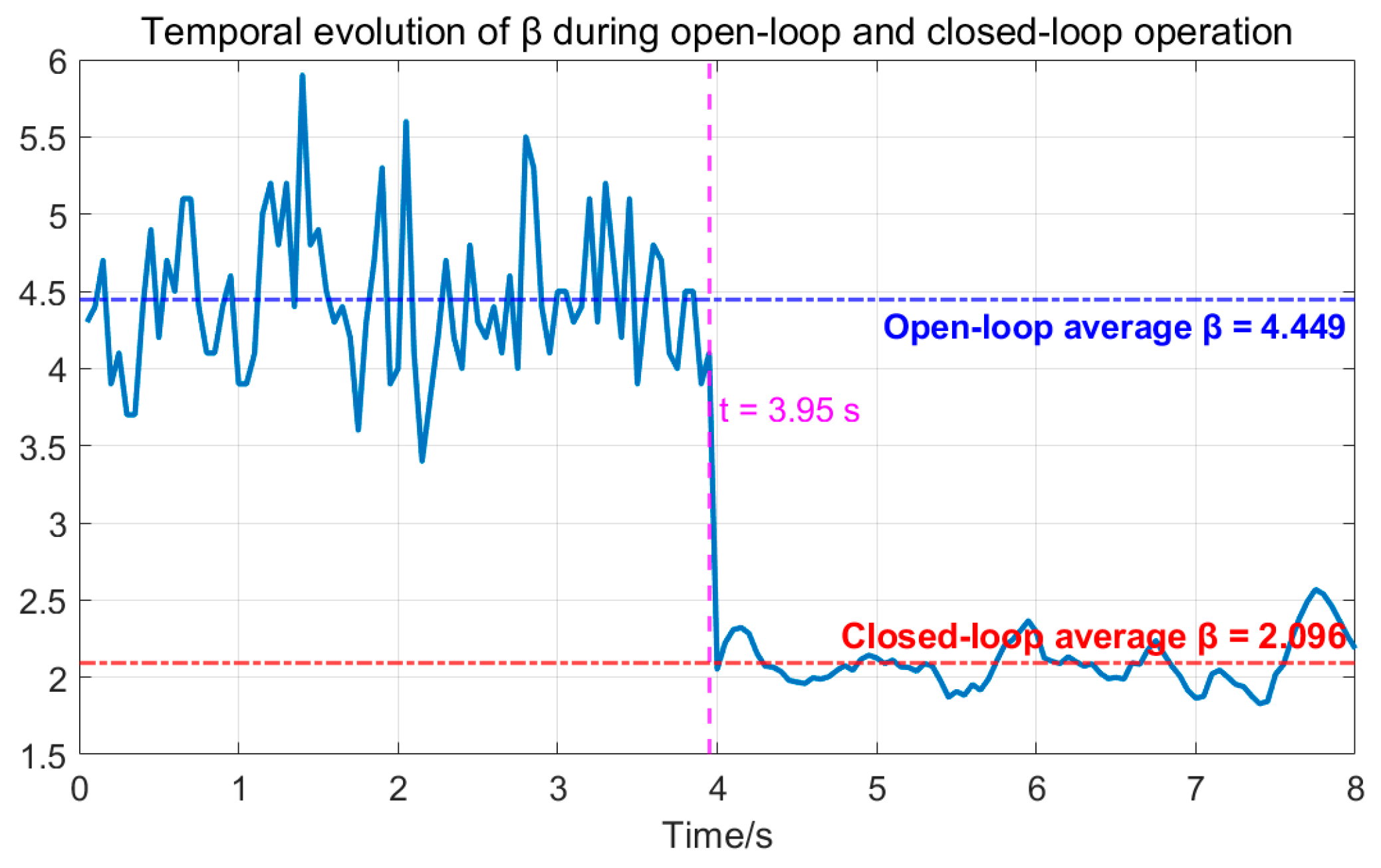
Figure 15 presents the curve of the beam quality factor β during the transition from open-loop to closed-loop at $t=3.95\mathrm{s}$. The average β value improved from 4.449 to 2.096, representing an improvement factor of approximately 1.12.

In addition, a significant reduction in the temporal variance of β is observed in the closed-loop state compared with the open-loop state. The large fluctuations in the open-loop state reflect the dynamic jitter induced by the simulated atmospheric turbulence ($r_0\approx 2\mathrm{cm}$). The stabilization of the β curve after $t=3.95\mathrm{s}$ demonstrates that the proposed system provides high detection accuracy and sufficient correction bandwidth to suppress the dynamic jitter. This indicates the system stability under strong turbulence conditions.

Overall, these experimental results verify the effectiveness of the proposed compensation method for laser array atmospheric propagation, demonstrating its robust capability to significantly enhance the far-field energy concentration of a multi-beam laser array.

5. Conclusions

This paper presents a tip–tilt aberration correction scheme tailored for laser array atmospheric propagation based on a cooperative beacon, which incorporates a modified SHWFS and an SDM. By utilizing the return wavefront from the cooperative beacon, the proposed system enables direct and independent measurement of the tip–tilt aberration for each sub-beam and performs real-time closed-loop correction.

Simulation results for different numbers of sub-beams (N = 7, 19, and 37) under atmospheric coherence length $r_0=5\mathrm{cm}$ demonstrate the robust scalability and high precision of the proposed system. Following correction, the average SR increased to 0.920 (N = 7), 0.959 (N = 19), and 0.973 (N = 37), while the average β was reduced to 1.374 (N = 7), 1.264 (N = 19), and 1.246 (N = 37). In terms of adaptability of turbulence conditions, the system exhibits high robustness across varying coherence length in the simulation. Under conditions of weak-to-moderate turbulence ($r_0>8\mathrm{cm}$), the corrected metrics consistently approach the diffraction limit.

Even under severe turbulence ($r_0=2\mathrm{cm}$), experimental validation using a 30-beam laser array confirms that this system remains capable of concentrating scattered far-field spots into a stable and high-intensity synthesized spot, thereby achieving a significant improvement in energy concentration. Additionally, the consistency of correction performance as the number of sub-beams increases from 7 to 37 confirms the excellent scalability of this approach.

Although the current scheme excels at compensating for the dominant tip–tilt aberrations (accounting for approximately 87% of the phase variance), the performance of the system is inherently constrained by the dynamic range of the sub-apertures and the presence of high-order aberrations under extremely strong turbulence conditions. Future research will focus on the integration of high-order wavefront sensing and the exploration of hybrid control strategies to further enhance the performance of the system in non-Kolmogorov atmospheric environments.

Overall, this study demonstrates that efficient suppression of the turbulence-induced tip–tilt aberration in the laser array can be achieved through direct wavefront sensing and correction using cooperative beacons. The proposed technique provides a practical and scalable solution for improving beam quality and energy concentration in high-energy laser systems operating in atmospheric environments.