Article

Validation of a Single-Image Inverse Rendering Setup for Optical Property Estimation in Turbid Materials


Institute for Laser Technologies in Medicine and Metrology at the University of Ulm, Helmholtzstr. 12, D-89081 Ulm, Germany
*
Author to whom correspondence should be addressed.
Photonics 2026, 13(3), 242; https://doi.org/10.3390/photonics13030242
Submission received: 28 January 2026 / Revised: 19 February 2026 / Accepted: 27 February 2026 / Published: 28 February 2026
(This article belongs to the Special Issue Computational Optical Imaging: Progress and Future Prospects)

Abstract

This work presents an experimental validation of a physics-based inverse rendering method for determining the reduced scattering and absorption coefficients of turbid materials in arbitrary shape from a single image per wavelength. Based on our previously published theoretical inverse rendering framework, we constructed and experimentally characterised a wavelength-selective measurement setup to realise and validate the method under real acquisition conditions. By accurately modelling the spectral behaviour and angle-dependent transmission of the employed bandpass filters, we ensured a close correspondence between captured and simulated reflectance. The method was evaluated on three silicone materials, beginning with simple cube geometries and later extending to a complex Einstein bust. Relative to integrating-sphere reference data, the recovered optical properties exhibit maximum absolute errors of approximately 4–10% for reduced scattering and 5–10% for absorption for the cubes, and 16–19% and 16–22%, respectively, for the bust. Forward renderings based on the recovered coefficients achieve CIE Δ E 2000 values below 1 for the cube and below 2 for the complex geometry when compared with photographs. Additionally, we demonstrated that the approach can be applied using a common commercially available RGB camera, recovering optical parameters from each RGB channel, albeit with increased errors due to the camera’s broad spectral channels. Overall, our method enables the recovery of optical properties and the creation of accurate digital twins for objects of arbitrary shape using comparatively simple hardware, including common commercially available RGB cameras. This broadens its applicability to practical scenarios such as process monitoring and digital twinning when appearance, rather than precise material parameters, is the primary focus.

1. Introduction

The perceived colour of an object arises from a combination of its intrinsic optical properties, geometric form, and the illumination conditions under which it is viewed. Accurately rendering such materials using optical property-based models [1,2] requires precise determination of the fundamental parameters of the radiative transfer equation (RTE) [3]: the absorption coefficient μ a , the scattering coefficient μ s , the refractive index n, and the scattering phase function, which is commonly characterised by the anisotropy factor g [4]. Techniques for determining absorption and reduced scattering coefficients, μ s = μ s ( 1 g ) , include integrating-sphere measurements [5,6] and goniometric methods [7]. Although these approaches offer high measurement accuracy, they often impose stringent requirements on sample preparation. For example, the integrating-sphere method [6,8,9,10,11] typically necessitates multiple plane-parallel samples of varying thicknesses for characterising materials having spectrally strongly different optical properties. Comparable preparation demands and reliance on specialised equipment likewise limit the applicability of other traditional techniques [12,13].
Previously, in [14], the optimisation strategy, filtered detection model, and convergence behaviour of an alternative approach for determining the scattering and absorption coefficients were analysed under simulated conditions. The present work translates the theoretical formulation into a physically realised measurement setup and aims to validate its performance experimentally. This approach requires only a single image per examined wavelength to recover both the reduced scattering and absorption coefficients. Furthermore, in contrast to other methods, if the object’s geometry is known, neither further sample preparation nor a certain shape of the sample, e.g., thin slabs, are required. The method is based on a Graphics Processing Unit (GPU)-accelerated, fully physics-based, tetrahedral rendering framework [1], in which light propagation through turbid media is accurately modelled by numerically solving the radiative transfer equation (RTE) [3]. Our framework allows us to precisely compute the different influences of scattering and absorption coefficients on the reflectance, especially on edge effects and translucency. This is the most important feature of our method as it allows us to separate the contributions and optimise both coefficients from one image at the same time, using a Levenberg–Marquardt (LM) algorithm [15].
In [14], we discussed previous related works in detail. Thus, only a brief summary is provided here. Several studies have investigated inverse approaches for recovering optical properties [16,17]. These include methods based on single-scattering models [18,19] as well as those derived from the diffusion equation [20,21]. Other related works that use more complex light transport models, like Pranovich et al. [22], analysed thin sample slabs using spectrometer measurements, while Elek et al. [23,24] employed a similar thin-slab configuration combined with camera-based reflectance acquisition across the three colour channels to characterise a set of 3D printing inks. Iser et al. [25] extended this concept to enable spectral resolution and further refined their approach in [26], where the recovered optical properties were compared with our previously reported measurements [2], demonstrating good agreement. Gkioulekas et al. [27] utilised a hyperspectral imaging setup to capture both reflectance and transmittance data, thereby recovering optical properties across three spectral channels. Chen et al. [28] demonstrated that comparable results can be achieved using ordinary RGB images, although their method requires at least three input images. Closely related work by Deng et al. [29] further recovers both geometry and appearance of complex objects through an inverse bidirectional scattering–surface reflectance distribution function formulation. Depending on the specific scene configuration and material characteristics, additional inverse approaches have been presented in other studies [30,31,32].
In this work, we experimentally realise and validate the previously proposed inverse rendering framework [14] by constructing and characterising a dedicated measurement setup and used it to measure several optical phantoms [33], first in a simple cube shape and then with more complex geometry, to recover their reduced scattering and absorption coefficients. As proposed, we built a detection setup that uses a set of bandpass filters to detect a defined wavelength range with the camera. This input data then allowed us, for each filter, to recover the pair of coefficients that best matched the optical properties required to reproduce the recorded reflectance. To achieve this, we fully characterised the spectral behaviour of the camera and the set of narrow-band optical bandpass filters. Furthermore, we incorporated the dependency of the filters on the angle of incidence (AOI) of the incoming light and the resulting variation in transmission loss. This allowed us to characterise the detection setup sufficiently well to achieve a good match between our simulation and the captured images. Forward renderings with the obtained optical properties were then computed, and their CIE Δ E 2000 colour difference [34] to the original camera images was evaluated. The CIE Δ E 2000 metric [34] quantifies the perceptual difference between two colours within the approximately perceptually uniform CIE L*a*b* colour space, incorporating corrections to better align numerical differences with human visual perception. Smaller values indicate closer visual agreement, and differences below approximately 2 are typically regarded as visually minor and near the threshold of perceptibility for most observers under standard conditions. Lastly, as described in [14], we used RGB camera images as input data. From a single RGB image, we extracted the coefficient pairs for the three wavelengths associated with the three colour channels.

2. Materials and Methods

In this section, we briefly revise the theory and the assumptions made in [14]. This includes the Monte Carlo (MC) algorithm used to render light transport, the LM fitting algorithm, and the characterisation of the used camera and filters. We then explain in more detail the experimental setup used to capture the images that served as reference for this study.

2.1. Light Transport Modelling via Monte Carlo Simulation

A GPU accelerated MC simulation was used to model physics-based light transport through turbid media as a numerical solution of the RTE. Within this MC framework, light propagation is represented by individual energy packets, referred to as photons, which are traced through the medium under variable lighting and viewing conditions. This in-house developed software is implemented in OpenCL [35] to enable execution on multiple GPUs. The simulations are controlled via a Python python312 interface, which launches independent OpenCL kernels on each GPU. All eight NVIDIA A10 GPUs (NVIDIA Corporation, Santa Clara, CA, USA; NVIDIA A10 GPU, 24 GB GDDR6 VRAM) used in this study are installed within the same server. Since the Monte Carlo photon simulations are statistically independent, no inter-GPU communication is required. Photon batches are distributed across devices and the resulting statistics are aggregated after kernel execution. The optical properties of the observed medium, namely the scattering and absorption coefficients, the refractive index, and the scattering phase function, fully describe it in the context of the RTE. In this case, the Henyey–Greenstein phase function [4], characterised by the anisotropy factor, was chosen as the scattering phase function. Interactions between media with different refractive indices were handled using the Fresnel equations [36]. The simulation computes the light transport through a tetrahedron-based 3D scene that incorporates the geometry of the objects and their material distribution. To improve computational efficiency, backward photon tracing from the detector to the light source was employed. Photon weights were reduced after each scattering event, and photons were terminated once their weight dropped below a predefined threshold. Additionally, a maximum number of scattering events per photon was imposed. As demonstrated in [1,2], this approach produces rendered images exhibiting good agreement with actual photographs, quantified using the CIE Δ E 2000 colour difference metric [34]. A more detailed description and previous applications can be found in [1,2,14].

2.2. Parameter Recovery via Levenberg–Marquardt Fitting

The inverse optimisation procedure employed in this work is identical to the LM–based framework introduced and analysed in detail in [14]. No modifications to the optimisation strategy, cost function formulation, or convergence criteria were made. For completeness, the main steps of the procedure are summarised below. Using the MC simulation, we can inversely recover the scattering and absorption coefficients from a single image as follows. Through the MC simulation, we obtain detailed information on the light transport from the source, through the object, to the detector. We then vary the optical properties in question to match the recorded image within the context of an LM algorithm. As described previously, we used the gradient-based framework provided by [15]. The optimisation minimises the root-mean-square error between simulated and measured reflectance values. To improve computational performance, we employed scaling relations in our simulations [37,38] to compute the required gradients. In each iteration of the LM algorithm, between 10 9 and 5 × 10 9 photons were simulated. Depending on the geometric complexity of the object, this resulted in computation times ranging from 30 s to 150 s using a setup with eight NVIDIA A10 GPUs. As previously mentioned in [14], the initial parameter choice was handled by first performing a pre-fit with arbitrary starting values of μ a = 0.5   m m 1 and μ s = 1   m m 1 to rapidly explore the parameter space and identify a region close to the optimum. The final fit was then initialised in this region using more conservative settings to ensure stable convergence, with an average of approximately 30 iterations performed. With this robust inverse method, the best-fit results return the scattering and absorption coefficients of the examined medium from one image at a defined wavelength. Repeating this method then allowed us to recover the spectrum of the optical properties.

2.3. Characterisation of the Camera and the Filters

We required precise information on the camera’s sensitivity, especially when paired with the filters used in this study. To measure the camera’s spectral sensitivity, we employed a setup in which a monochromator illuminated an integrating sphere, whose port was then imaged by the camera. Simultaneously, the power at the port was measured with a photodiode. From the photographs of the port, we extracted the detected intensity, which, in relation to the photodiode measurements, allowed us to compute the camera’s wavelength-dependent sensitivity. These measurements were performed covering the wavelength range of 380 n m to 720 n m with 1 n m increments. The resulting curve of the unobstructed camera is shown in Figure 1. The same measurement was then performed with the filters placed in the light path before the camera, and the measurement was repeated for each filter. The resulting sensitivity curves, one per filter, are also shown in Figure 1, displayed together but clearly distinguishable by the locations of their prominent sensitivity peaks at the filters’ centre wavelengths.
Next, we examined the transmission characteristics of the filters in more detail. Since the transmission loss is influenced by the AOI, and since we capture a fixed field of view (FOV) through the filters, we expected varying transmission values across the FOV. The manufacturer of the filters provided measurements of the transmission, T λ 0 ( λ i , θ j ) , as a function of wavelength and AOI for each filter from 350 n m to 750 n m with an angular resolution of 1°. For each filter, we extracted the maximum transmission via
T λ 0 ( θ j ) = max i T λ 0 ( λ i , θ j ) ,
where λ 0 is the central wavelength of the filter, and θ j is the AOI. Next, we mapped the per-angle transmission loss onto the angular distribution of the camera’s FOV. For a pinhole camera model, this mapping is well defined. Using the distance from the detector to the pinhole, d p , and a pixel pitch of p x , the physical coordinates x k and y l of pixel p ( k , l ) are given by
x k = ( k c x ) p x , y l = ( l c y ) p x ,
where c x and c y are the coordinates of the FOV centre. The AOI-per-pixel mapping then reads
θ k l ( d p ) = arctan r k l d p ,
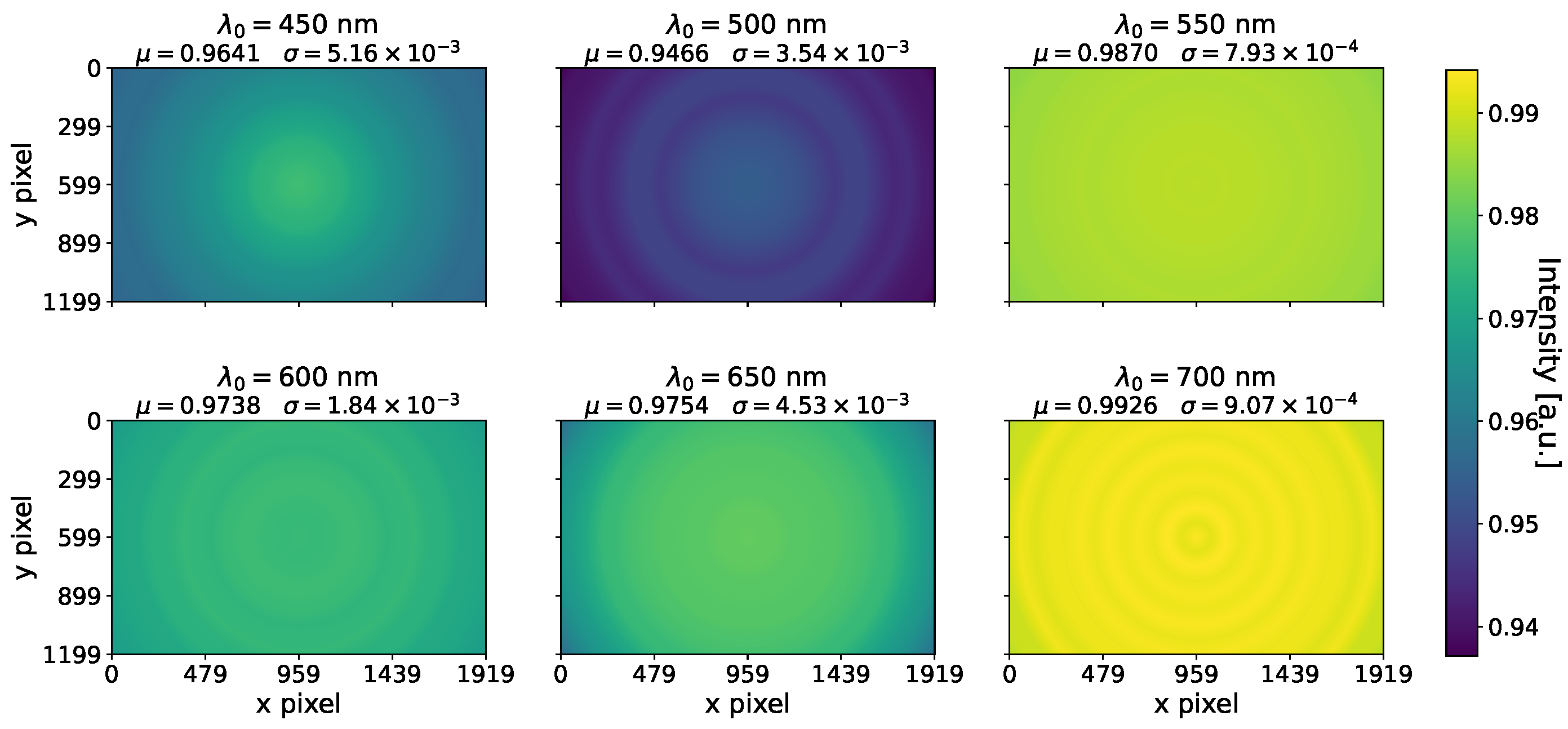
where we have used the radial distance of the pixel to the middle of the FOV, r k l = x k 2 + y l 2 . In this work, the camera had the following specifications: d p = 25   m m , p x = 0.0586   m m , and detector pixel dimensions of n x = 1920 px and n y = 1200 px. With this information, we computed the per-pixel transmission loss map M λ 0 ( k , l ) , shown in Figure 2, in the camera’s FOV for each filter via
M λ 0 ( k , l ) = T λ 0 ( θ k l ( d p ) ) ,
where we additionally quantify the overall magnitude of each map’s correction via the mean μ of the transmission loss and its standard deviation σ , shown in the individual titles of the maps in Figure 2. Since the transmission values remain above approximately 0.94 for all wavelengths, the per-pixel correction amplifies measurement noise by less than about 6% in the worst case.
The filter-corrected image data I corr , λ 0 ( k , l ) was obtained by applying these maps to the captured images by computing
I corr , λ 0 ( k , l ) = I λ 0 ( k , l ) M λ 0 ( k , l ) ,
where I λ 0 ( k , l ) is the captured image data of the ( k , l ) th pixel with the filter specified by λ 0 , which models the filters used in our setup and improves the match between simulation and photograph. The ringed pattern observed in the transmission loss maps is consistent with the angle-dependent centre wavelength blue shift inherent in thin-film interference bandpass filters. As the angle of incidence varies across the field of view, the effective bandpass shifts relative to the illumination wavelength, producing concentric regions of slightly increased and decreased transmission.

2.4. Setup of the Photobox and Filtered Camera

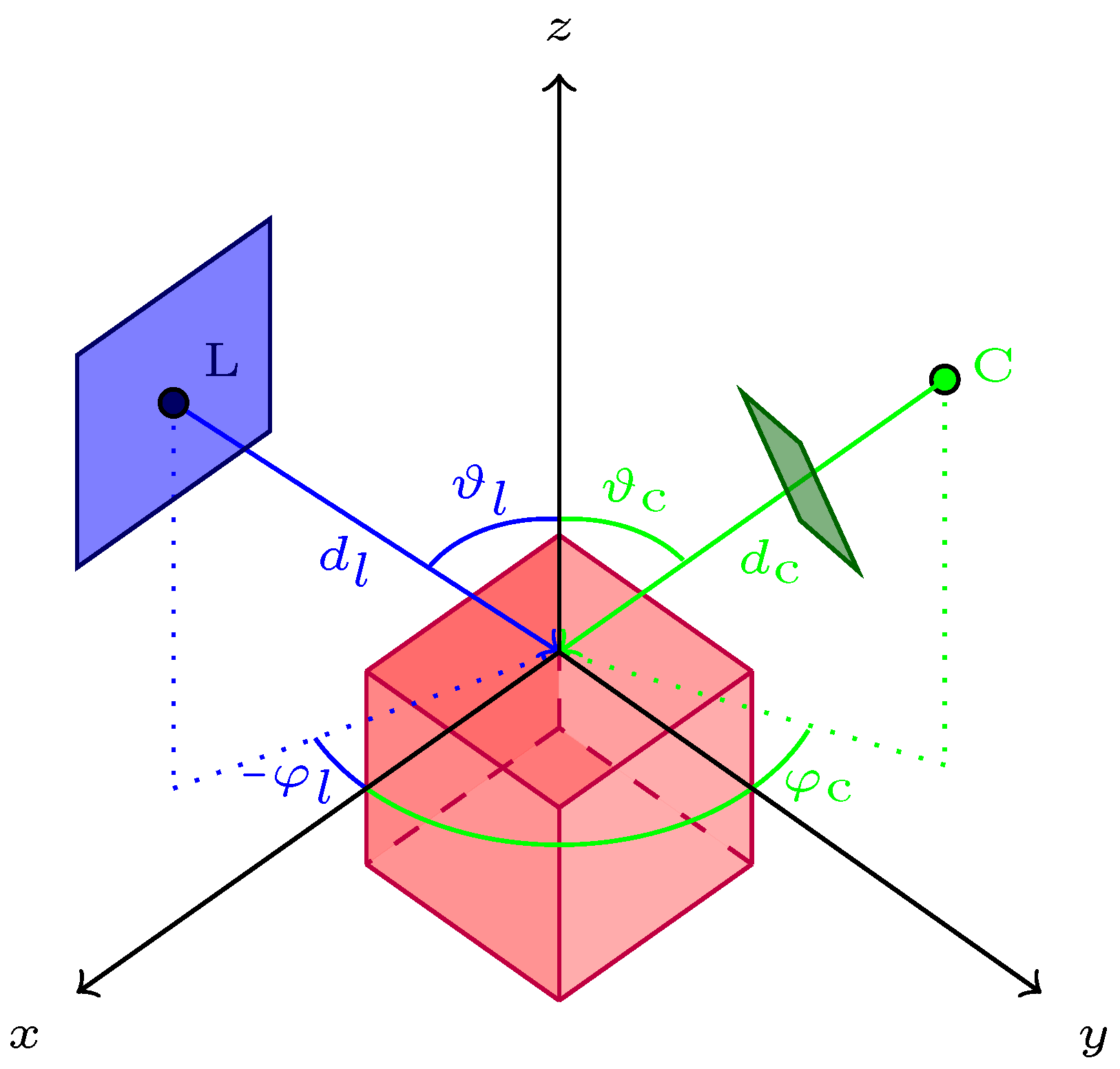
To record the necessary reference images for this study, we used the filtered camera setup inside a photobox. Firstly, we describe the photobox, schematically shown in Figure 3.
The photobox was illuminated by an LED panel whose spectral intensity distribution was fully characterised [1]. Its spectral intensity curve is shown in Figure 1. The detection unit consisted of a standard IDS camera (IDS Imaging Development Systems GmbH, Obersulm, Germany; U3-3060CP-M-GL Rev.2.2) with a 25 mm objective (Edmund Optics, Barrington, NJ, USA; 25 mm Focal Length Lens, 1” Sensor Format, #63-246), in front of which a set of hard-coated bandpass filters (Thorlabs, Newton, NJ, USA; Hard-Coated VIS/NIR Bandpass Filter Kit, FKBV10) was mounted. The filters were held in a motorised filter wheel (Edmund Optics, Barrington, NJ, USA; USB/RS-232 Motorised Filter Wheel, #23-646) that allows rotation through the filters without altering the camera’s position. This compact setup enables the capture of images at different wavelengths defined by the filters’ centre wavelengths. For this study, we used filters with a full width at half maximum (FWHM) of 10 n m and centre wavelengths from 450 n m to 700 n m in nearly 50 n m increments. Minor shifts in the centre wavelengths of less than 2 n m were observed when we characterised the filters, c. f. Figure 1. Measurement at 400 n m was not possible due to the near-zero intensity of the light source at that wavelength, as shown in Figure 1, but would otherwise follow the same procedure as the other measurements. Thus, we sample the complete visible spectrum, missing only the information of the filter at 400 n m .
As explained in [14], we require the transmission profile of the filters in combination with the camera sensitivity to accurately simulate the image’s intensity data I camref . From [14], we recall
I camref ( λ 0 ) = [ λ 0 d , λ 0 + d ] d λ I ( λ ) G λ 0 ( λ ) C ( λ ) L ( λ ) [ λ 0 d , λ 0 + d ] d λ G λ 0 ( λ ) C ( λ ) L ( λ ) ,
where I ( λ ) represents the intensity from the MC simulation at wavelength λ , λ 0 the centre wavelength, and d = 3 σ the range implied by the FWHM of the filter with shape G λ 0 ( λ ) . L ( λ ) denotes the spectral intensity distribution of the light source, and C ( λ ) the camera’s spectral sensitivity. In [14], we chose the shape of the filters to be ideally Gaussian, but now we can use the measured product of C ( λ ) with the filter’s behaviour directly. This gives us a combined filter function F λ 0 ( λ ) per filter and Equation (6) becomes
I camref ( λ 0 ) = VS d λ I ( λ ) F λ 0 ( λ ) L ( λ ) VS d λ F λ 0 ( λ ) L ( λ ) ,
where we integrated over the visible spectrum (VS) to account for all contributions of the filters whose shapes are now non-ideal. Equation (7) was used in this work to match the simulated reflectance with the recorded images.

3. Results

3.1. Validation of the Measurement Setup

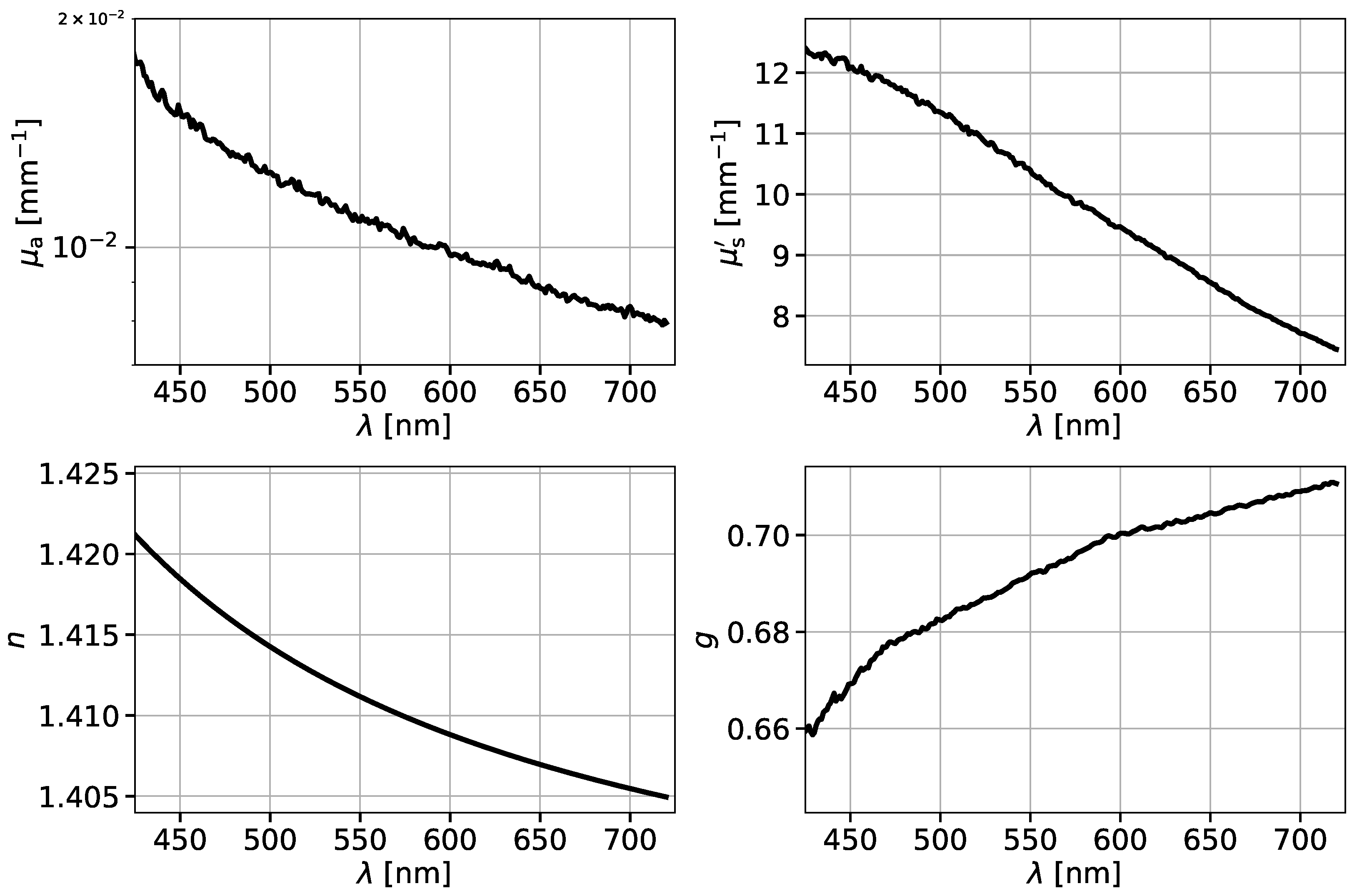
To verify the accuracy of our measurement setup and its agreement with our simulation, we recorded an optical phantom, a silicone mat with dimensions of 20 c m × 20 c m × 0.6   c m , created in-house [33], with precisely characterised optical properties, as shown in Figure 4, and compared it with forward renderings from our MC simulation. The scattering and absorption coefficients were determined using an integrating-sphere setup, the refractive index using an ellipsometer, and the anisotropy factor via collimated transmission in combination with an integrating sphere.
Furthermore, similar to [1,2], we used this phantom to calibrate the brightness scaling factor of our measurement setup. This scale factor was subsequently used to match the brightness between the recorded images and the simulation. We recorded this grey silicone mat at a 45° viewing angle, with the light source also placed at 45° to the left; that is, we chose φ l = 0 , φ C = 90° and ϑ l = ϑ C = 45 ° , as defined in Figure 3. This configuration of illumination and viewing angle was shown to be the most suitable for acquiring the optical properties via the fit [14]. As described in Section 2.3, we recorded an image with each filter at 450 n m , 500 n m , 550 n m , 600 n m , 650 n m , and 700 n m . Each measurement was taken five times per wavelength and then averaged to reduce noise. These mean images were then corrected using the corresponding AOI transmission loss filter maps from Section 2.3 to improve the agreement between measurement and simulation.
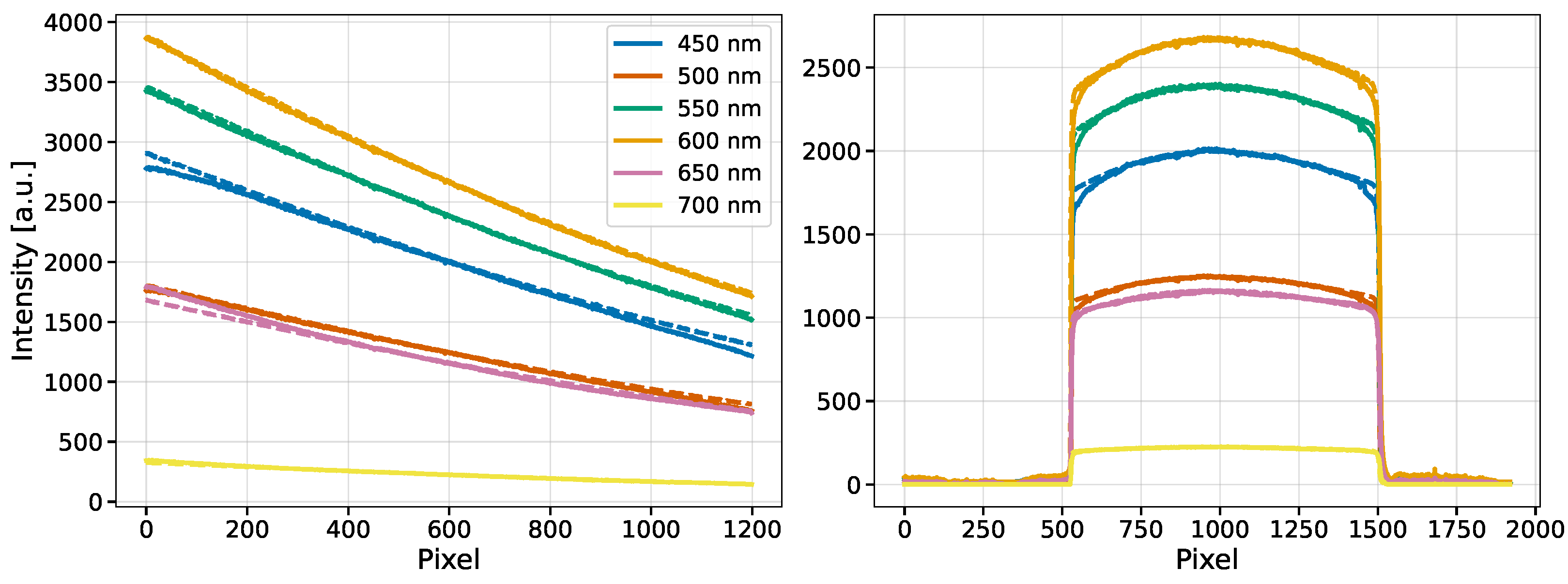
Next, the equivalent scene was computed in the simulation. We extracted the mean intensity from a 10 × 10 px region of interest (ROI) at the centre of both the simulated and recorded scenes and computed the brightness scale factor per filter s λ 0 = I cam I sim , where I cam and I sim are the mean intensities from the chosen ROIs. All subsequent simulations were then calibrated by multiplying with s λ 0 . In Figure 5, we show the comparison between the recorded and simulated calibration mat by taking vertical and horizontal slices through the middle of the scenes. These mean-intensity curves represent the average of the middle pixel line ±5 pixel lines for each orientation.
Both the horizontal and vertical image lines show good agreement between the photographs and the simulation. We observe minor deviations towards the edges of the object, e.g., at pixels 500 and 1500 in the vertical image lines. These deviations arise from imperfections at the edges of the silicone mat, residual misalignment of the object in the photobox, general errors introduced by the photobox due to reflected light and misalignment of the camera and light source, and inaccuracies of the optical properties used in the simulation. However, these errors have much less influence in the centre of the scene, which we use for calibration and, in the following results, for fitting the optical properties. The modelling of the camera and filter setup therefore provides a very robust basis for the results presented here. As a general remark, we mention that the model relies on a small number of simplifying assumptions. In particular, while angle-dependent effects are corrected using manufacturer-provided measurements, the filter response is assumed to be radially symmetric, and secondary scattering or reflection processes, such as light reflecting between the camera lens and the filter, are not explicitly included. Lastly, we note that the recorded images at 700 n m show considerably lower signal than the other wavelengths due to the low intensity of the light source, c.f. Figure 1, and are thus noticeably noisier. This can be seen in the comparison of the overall values of the image lines in Figure 5.

3.2. Recovering Optical Properties from a Cube Geometry

After validating that our MC simulation matches our measurement setup, we recorded images of three silicone cubes, which were manufactured using the same techniques as the mat [33]. Again, for the photobox setup, we chose φ l = φ C = 0 and ϑ l = ϑ C = 45 ° , as defined in Figure 3. The optical properties of the yellow, red, and blue materials were previously determined using an integrating sphere and are shown as the solid black lines in Figure 6.
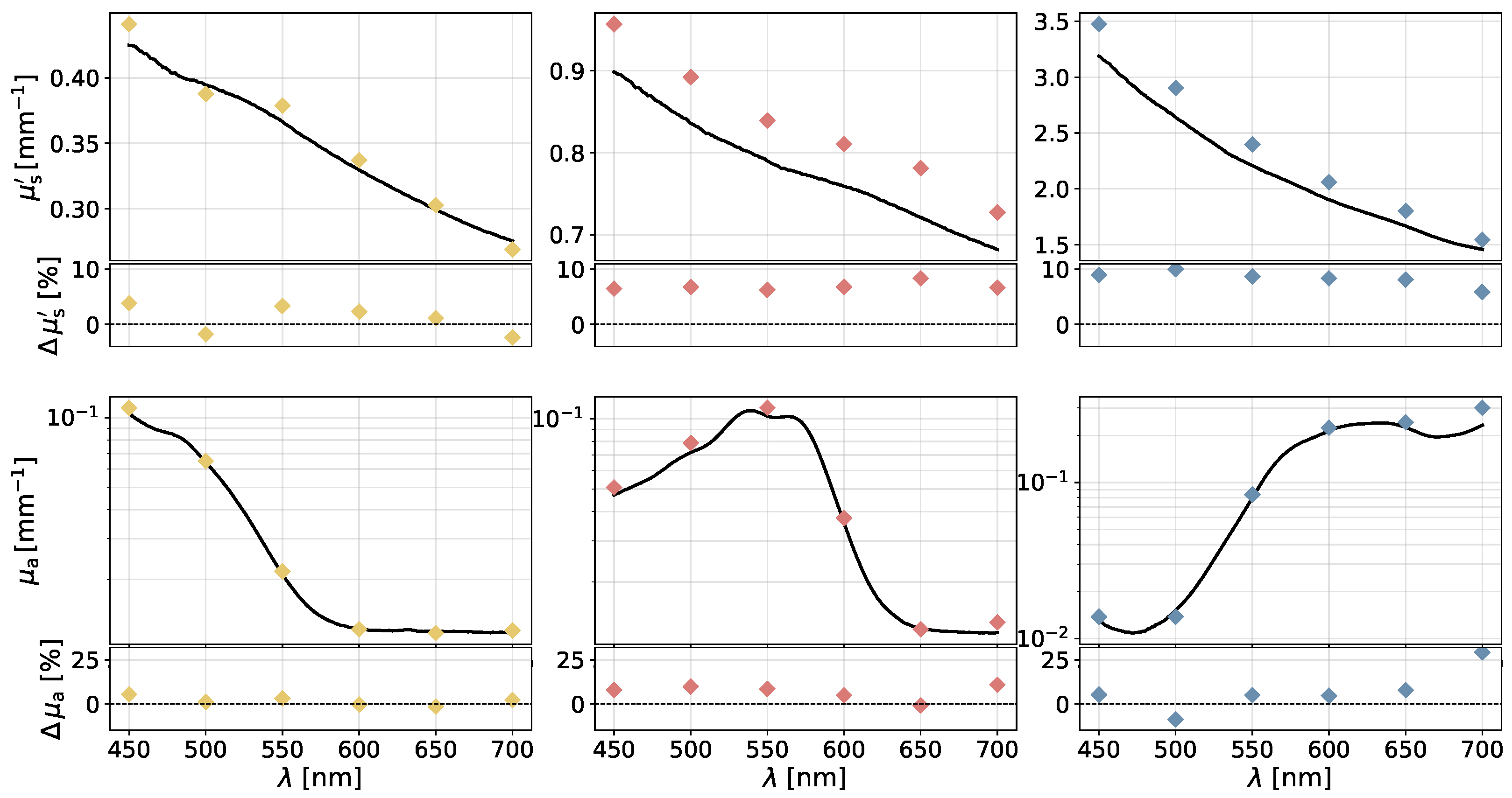
We then used these images to inversely recover the scattering and absorption coefficients of the three silicone materials. As mentioned in [14], it is sufficient to examine an image line through the object rather than the full image. In Figure 7, this image line is marked with red colour in the images in the second and third column. For the fit, we assumed that the refractive index and the phase function, via the anisotropy factor, of the materials are known, as shown in Figure 4, since the mat and the other objects are made from the same silicone base matrix. In this study, the cube geometry was analytically defined, and the more complex (Einstein bust, https://cults3d.com/en/3d-model/art/einstein-bust-3d-print-with-base-supported, accessed on 19 February 2026) geometry was directly obtained from the designer-provided 3D model used for fabrication, such that both shapes were known a priori. For objects with unknown geometry, established 3D acquisition techniques can be employed to obtain the required surface information with high accuracy [39,40,41,42,43]. We followed the procedure described in the fitting algorithm in [14]. The recovered optical properties for each filter, as well as the relative differences when compared with the reference values, are shown in Figure 6. For the yellow and red materials, we observe errors below 10%, with maxima of 3.8% for yellow and 8.3% for red. For the blue material, the error in the reduced scattering coefficient is closer to 10%, with a maximum of 10.2%. The absorption errors are slightly larger, with maxima of 5.2% for yellow, 9.8% for red, and 9.1% for blue. As analysed in [14], stronger intra-band variation of the absorption coefficient within the filter bandwidth makes its recovery more sensitive to spectral averaging effects, leading to slightly larger errors. We have omitted the values at 700 n m in this description, as the images recorded at this wavelength were significantly noisier than those at other wavelengths due to the low brightness, which makes convergence of the fit more difficult. In addition, values at and above approximately 700 n m have only a relatively minor influence on the visible appearance.
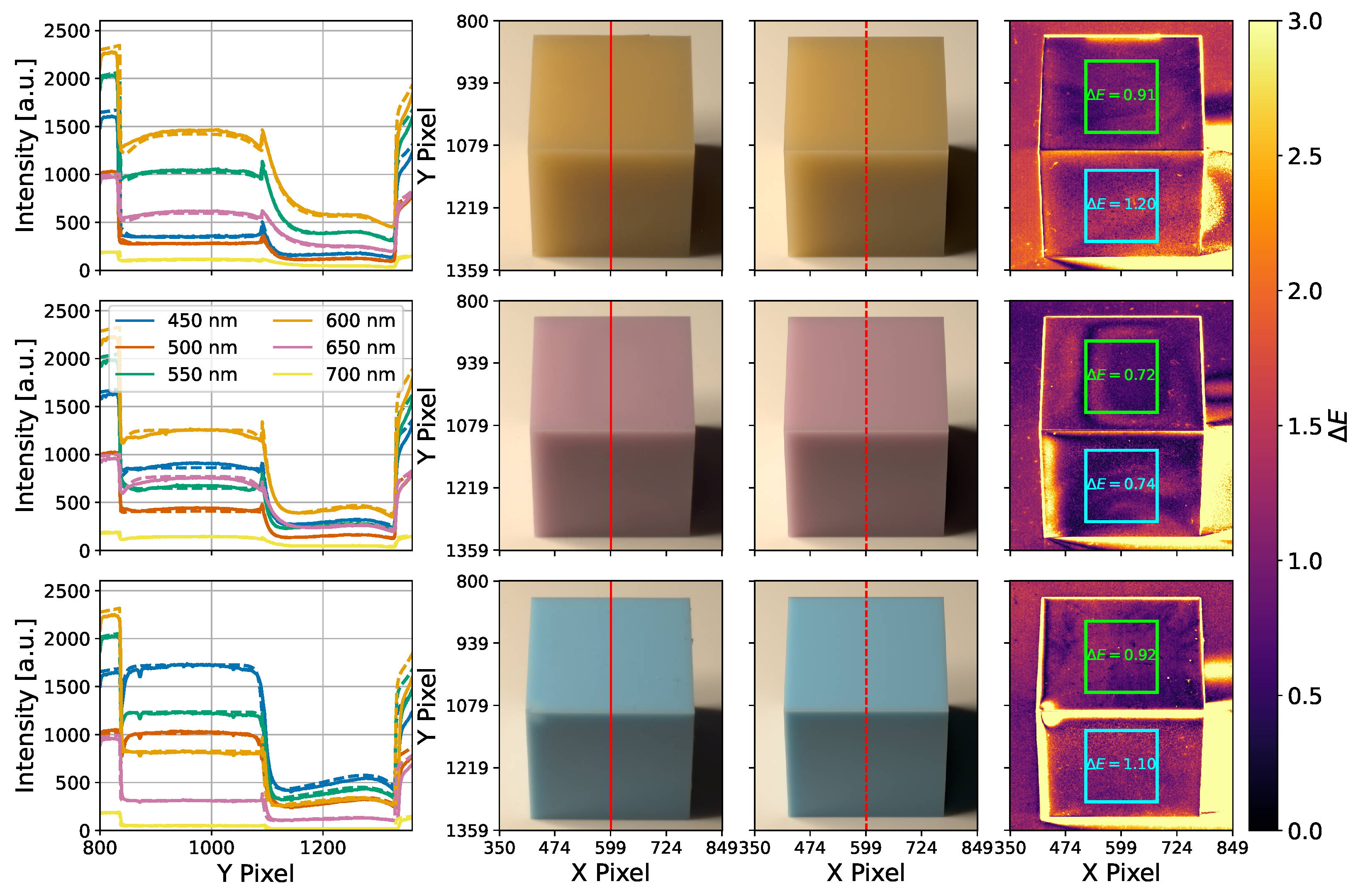
Next, we computed complete renderings of the cubes using the recovered optical properties and compared them with the recorded images via the CIE Δ E 2000 colour difference, as shown in Figure 7. As described in [1], we can use the simulation data at the six points defined by the central wavelengths of the filter set, together with the known spectral distributions of the light source and the camera, to compute a full image. Furthermore, the wavelength-resolved data of the simulation was weighted with the normalised intensity of the corresponding filter to account for the intensity relation between the filters, c.f. Figure 1. In this way, we transform our simulated data to match the raw camera images we have obtained. The same computations were performed with the simulated and recorded data to obtain the images shown in Figure 7. To establish defined bounds for interpolating the intensity between the six wavelengths and towards 400 n m , we chose the missing data point at λ = 400   n m to be a scaled-down version of the data at λ = 450   n m . The scaling factor f i was approximated by taking the ratio of the camera and light source curves at those wavelengths and reads f i = C ( λ 400 ) L ( λ 400 ) C ( λ 450 ) L ( λ 450 ) . This assumes constant values of the reduced scattering and absorption coefficients are between 400 n m and 450 n m , as the wavelength dependence of these coefficients is not known a priori. In future work, an additional filter located between 400 and 450 could improve the interpolation accuracy.
The mean Δ E values of the two cube sides facing the camera, computed within the marked ROIs in the Δ E maps, demonstrate very good agreement between simulation and measurement. For the majority of the cube faces, the mean Δ E values remain below 1 and are therefore visually indistinguishable. The front faces of the yellow and blue cubes show slightly higher values, with mean Δ E values of 1.1 and 1.2, respectively, which are still very close to the perceptual threshold. The Δ E values at the borders of the cube are larger as the very edge is not perfectly aligned and alignment errors of a few pixels remain. Another contributing factor is the imperfect surface quality of the phantoms. Although the cube surfaces are close to perfectly smooth, the edges exhibit small defects, e.g., blemished corners, as seen on the blue cube, and a striped pattern on the top surface of the red cube. Small heterogeneities during the mixing process of the cube materials remain and further alter the light propagation relative to the simulation that assumes perfect homogeneity. The shadowed regions in the images exhibit higher Δ E values, primarily due to the reduced signal levels, which increase the relative influence of errors and lead to a less favourable signal-to-noise ratio.
Furthermore, as before with the silicone mat, we examined the vertical image lines through the middle of both the photographs and the simulation. The resulting curves are shown in Figure 7 in the first column and are marked with red colour where they were extracted in the second and third columns. The remaining differences between the measured and simulated reflectance are the combined result of the measurement errors described in Section 3.1 and the errors introduced by the recovered optical properties shown in Figure 6. Nonetheless, we found a sufficiently close match between the photographs and the simulation, as demonstrated by the colour differences between the rendered and recorded images.

3.3. Recovering Optical Properties from a Complex Geometry

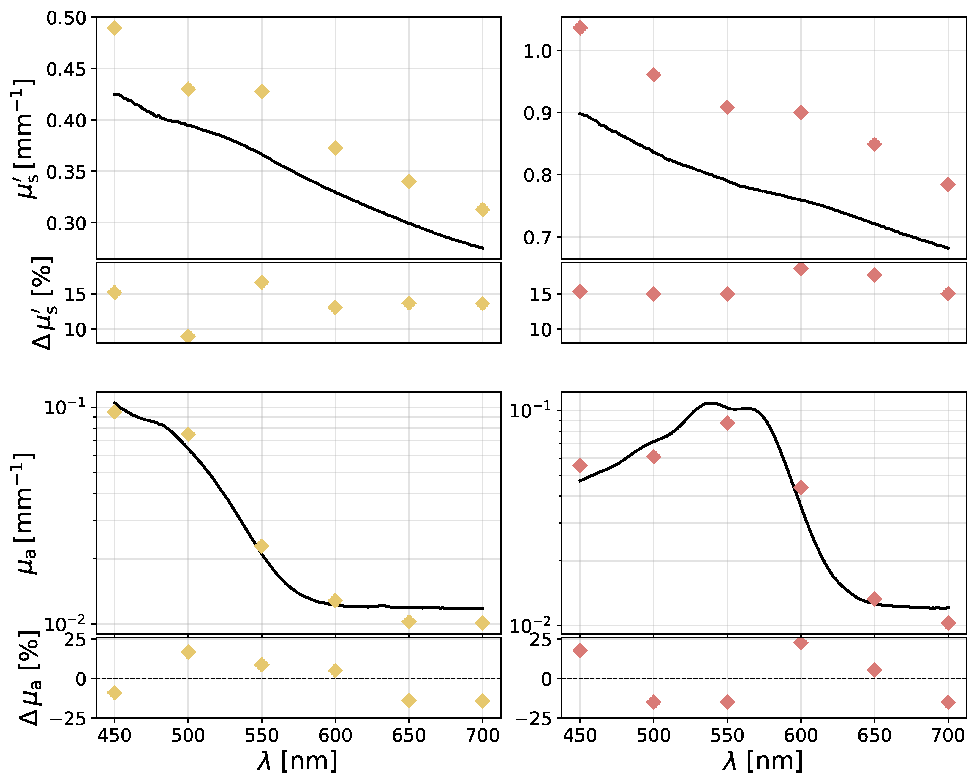
Next, we changed the geometry of the fit object to a more complex bust of Albert Einstein. The phantom was again cast from the silicone material in the colours yellow and red [1,33]. As before, we recorded images with each filter and extracted the fit reference data from a vertical middle image line. The recovered optical properties from the Einstein images are shown in Figure 8, together with the relative differences when compared with the scattering and absorption coefficients measured with an integrating sphere.
The relative differences are larger when compared with those obtained using the cube geometry due to the more complex geometry of the bust. For the yellow material, we observe maximum errors of 15.9% for the reduced scattering coefficient and 16.0% for the absorption coefficient. For the red material, they are 18.8% and 21.9%, respectively. The highly irregular shape made it more challenging to align the photographs and the simulation with the simple cube geometry than before. In addition, the increased geometric complexity introduces surface defects resulting from the manufacturing process, which influence light propagation. These factors compound with the previously discussed errors and lead to larger relative differences in the recovered optical properties.
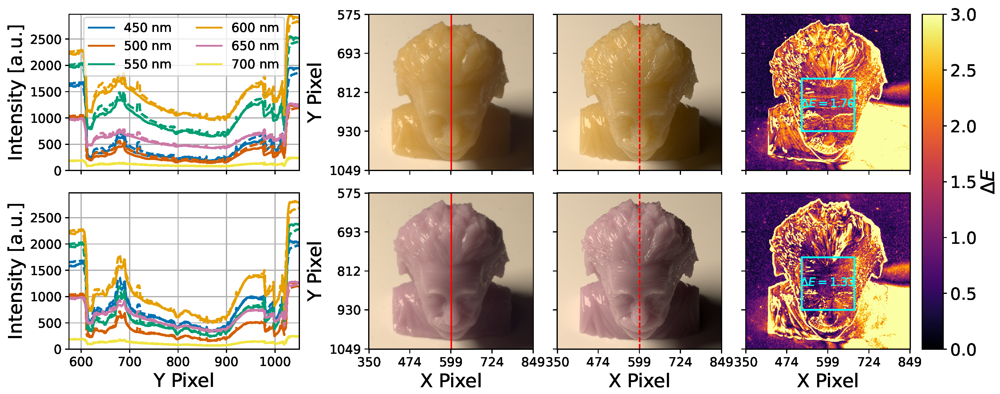
Again, we rendered images using the recovered scattering and absorption coefficients and compared them with the combined image from the filtered photographs, as shown in Figure 9. As can be seen in the images, the simulation is able to faithfully reproduce the most prominent features of the bust, including the facial characteristics and the hair structure. This is also reflected in the Δ E maps, which show extended regions with good colour agreement, such as on the forehead. Within the marked ROIs in Figure 9, acceptable colour differences of Δ E = 1.76 for the yellow material and Δ E = 1.33 for the red material were obtained. Nevertheless, the Δ E maps now exhibit local maxima where Δ E > 3 . These maxima occur at edges and in regions of high curvature. These detailed features of the bust are the most sensitive to alignment errors when the object is placed in the photobox. Furthermore, during the manufacturing process, these thinner and more elaborate parts of the phantoms are more susceptible to production errors, i.e., they often have a slightly different geometry than the ideal model. The negative used for casting the busts was 3D-printed and therefore limited in surface accuracy, which propagates to the silicone castings. The resulting surfaces show roughness and local defects, such as altered edge shapes.

3.4. Recovering Optical Properties from RGB Photographs

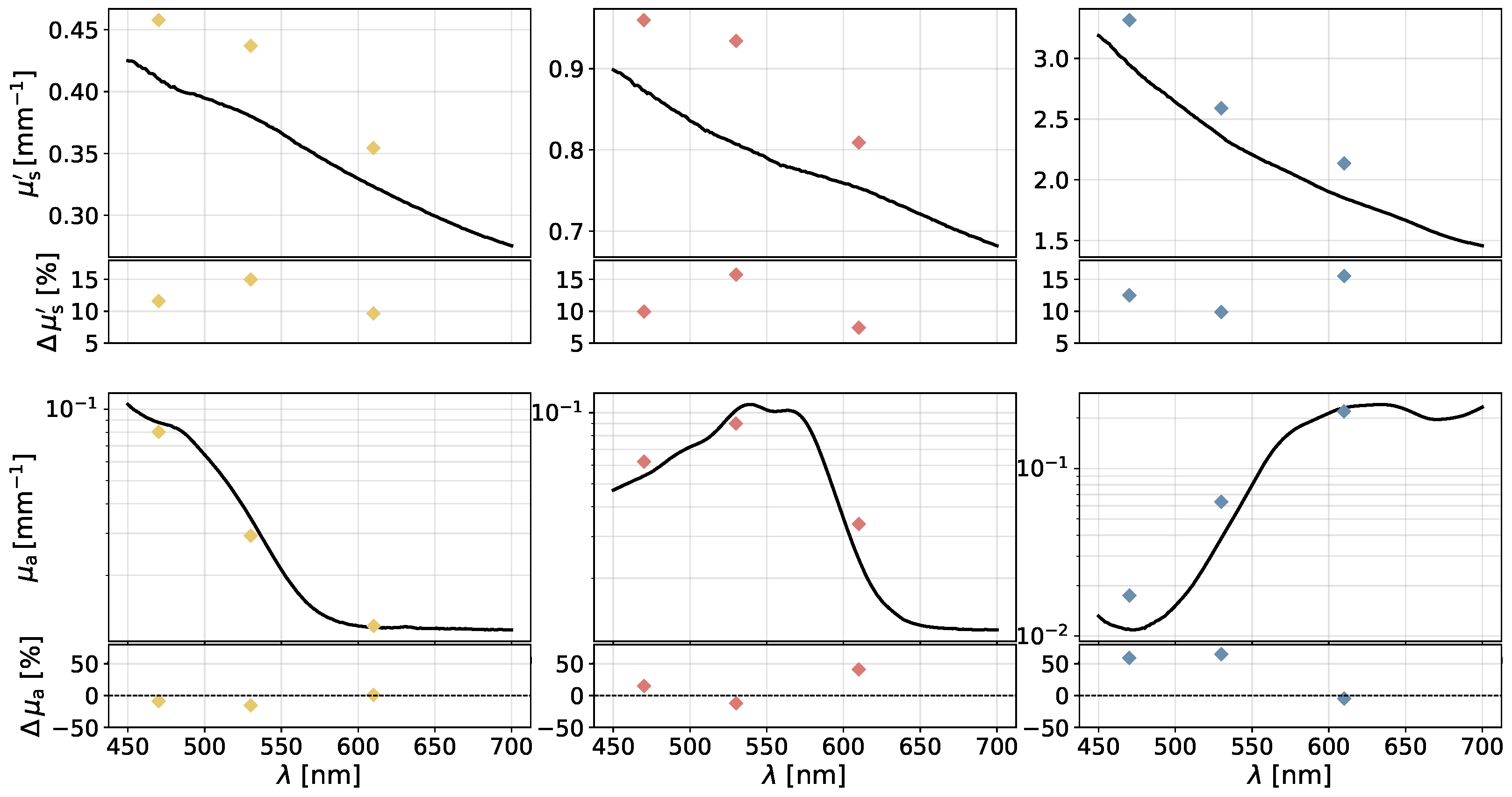
Lastly, we used ordinary RGB images as input data for our fitting method. We used the data previously recorded by Hevisov et al. [1], in which images of the three silicone cubes on the calibration mat were taken with a Nikon D7500. Our fit can then be applied as described in [14]; i.e., we assume that the RGB channels act as the filters through which we record the scene. In Figure 10, we show the recovered optical properties for the RGB channels, which we previously associated with the central wavelengths λ R = 610   n m , λ G = 530   n m , and λ B = 470   n m as well as FWHM values of FWHM R 65   nm , FWHM G 100   nm , and FWHM B 75 nm [14]. Thus, we obtained three pairs of scattering and absorption coefficients from a single image. However, this approach is limited by the fact that the intrinsic camera RGB channels are relatively broad. On the other hand, using a common commercially available RGB camera as the detector avoids errors introduced by additional optical elements such as bandpass filters. This also broadens the applicability of our method to any sufficiently well-characterised RGB camera.
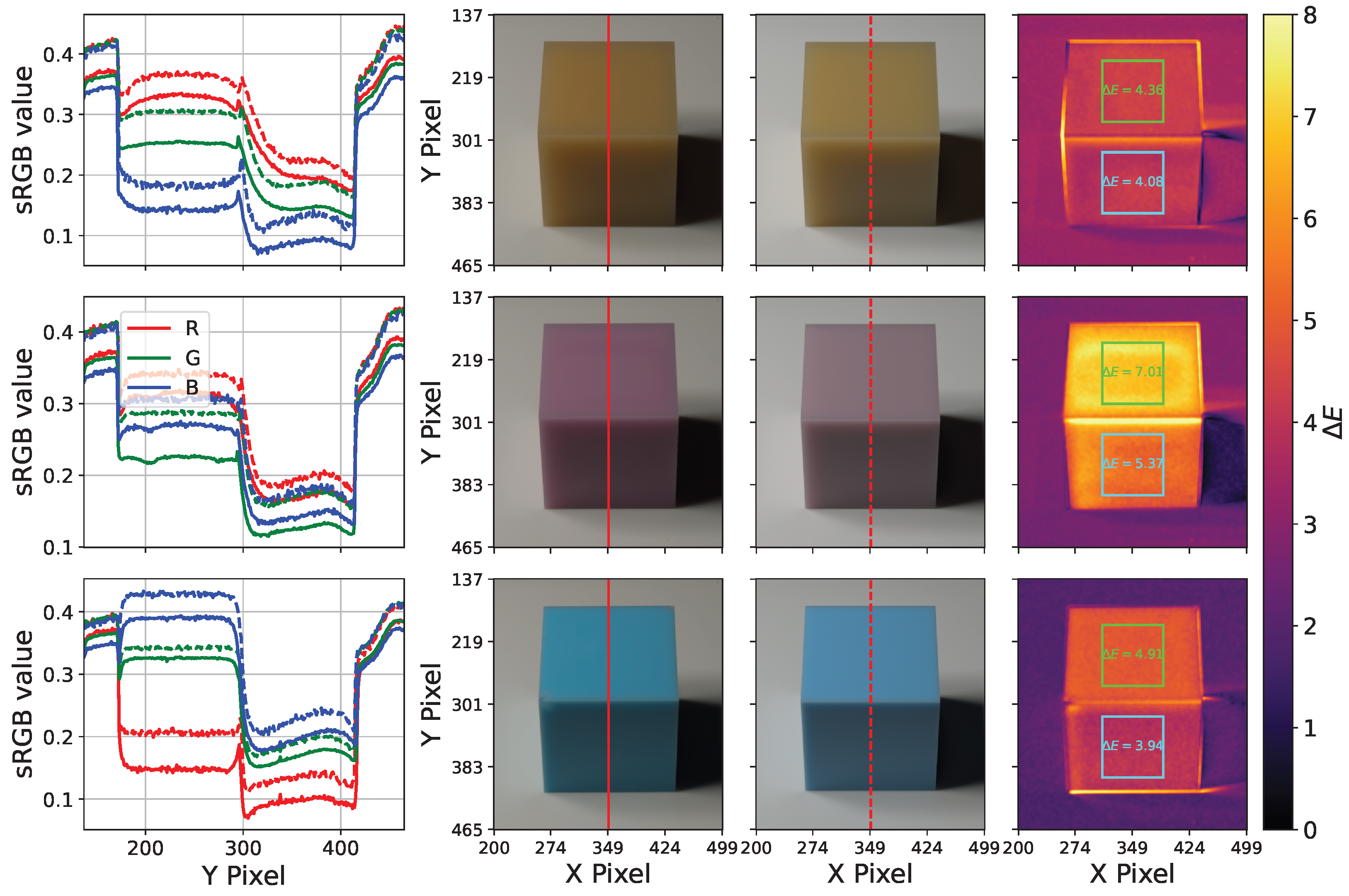
Once more, we rendered images using the recovered optical properties and computed the resulting colour differences. In this case, the deviations arising from the errors in the optical properties, the substantially wider integration intervals of the RGB channels, together with the sparse sampling of the visible spectrum using only three data points, lead to significantly larger colour differences, as shown in Figure 11. We used the framework established in [14] to generate a spectrally resolved image from the three recovered RGB data points. As in [14], spectral bounds at 400 n m and 700 n m are required for rendering across the visible range. To obtain these bounds, a pixel-wise linear interpolation model was applied. For each pixel, a linear spectral trend was determined using the recovered values at the three representative RGB wavelengths (470 nm, 530 nm, and 610 nm). The slope defined between the green channel (530 nm) and the blue or red channels was used to extrapolate the spectral behaviour toward 400 nm and 700 nm. This procedure yields five spectrally defined images (400 nm, 470 nm, 530 nm, 610 nm, and 700 nm), enabling interpolation across the visible spectrum under the assumption of locally linear spectral behaviour. While this represents a sparse spectral sampling, it provides a consistent approximation for RGB-based reconstruction. As expected, we now observe substantial deviations in both the optical properties and, consequently, in the colour difference when comparing the RGB images with forward renderings generated using the recovered properties. Again, we have marked the mean Δ E values in the ROIs on the cube’s main faces, this time with values that clearly indicate a noticeable colour difference. The RGB-channel data comparison is shown in the left column of Figure 11 and likewise demonstrates the mismatch caused by the deviations in the optical properties, which is a direct consequence of the wide filter intervals inherent in the intrinsic RGB channels.

4. Discussion

In this work, we presented a novel measurement setup for determining the reduced scattering and absorption coefficients from a single image. The setup consists of a common commercially available camera and a set of optical bandpass filters mounted in a photobox with a calibrated light source and defined angles of illumination and detection. We then used these these spectrally dependent images, given by the spectral characteristics of the used filters, to inversely recover the optical properties of three materials using our MC simulation. The geometry of the photographed objects, as well as the materials’ refractive index and scattering phase function, were preset. Deviations arising from errors in the assumed refractive index and anisotropy factor within the Henyey–Greenstein phase function were previously investigated in [14]. We examined three materials in cube geometry, two of which were additionally investigated in a more complex bust geometry of Albert Einstein. The recovered optical properties were compared with integrating-sphere measurements and exhibit maximum absolute errors of approximately 4–10% for reduced scattering and 5–10% for absorption for the cubes, and 16–19% and 16–22%, respectively, for the busts. The results obtained from RGB photographs show even larger errors, as expected, because the intrinsic RGB channels of the camera act as broad filters and therefore cannot achieve the precision provided by the 10 n m bandpass filters. In [14], we investigated in detail the influence of filter width on the fit results, as well as the ideally achievable performance using RGB channels.
We identify several reasons for the observed deviations of the optical properties obtained with the 10 n m filter setup. The main source of error is the imperfect alignment between the simulated and recorded scenes, including the relative positions and angles of the camera, light source, and object. This affects the light transport in general but is most prominently noticeable at the specular reflexes in regions with high curvature. In addition, the walls and components of the photobox are not perfectly black and therefore reflect light. Finally, the integrating-sphere measurements used as reference values also contain their own measurement errors.
We have shown that with a comparably simple setup we can recover the reduced scattering and absorption coefficients of samples that would be more difficult to measure with other methods due to their shape, such as with an integrating-sphere setup. In the present implementation, the optimisation was performed with a maximum of 40 LM iterations per wavelength to ensure robust convergence, although the optimum was typically reached after approximately 20 iterations. For the six-wavelength reconstructions shown here, this resulted in conservative upper bounds of approximately two hours for the cube geometry and up to eight hours for the more complex bust. Since each wavelength can be processed independently, the reconstruction could be parallelised, thereby reducing the effective time when sufficient hardware resources are available. Runtime optimisation was not the primary focus of this study, and further reductions are feasible through adaptive photon allocation and more elaborate early stopping strategies. Furthermore, our setup can also be used with a common commercially available RGB camera as the detector, further broadening its applicability. The measurement setup could also be used in process control environments, such as with objects on a slowly moving conveyor line. Within the motion-induced errors, the optical properties of the objects could be determined, the colour appearance rendered, and as we have shown, a digital twin could be created. Another application if the optical properties are not the main focus could be just the digital twinning of objects, which can then be placed into virtual environments. Future work should primarily focus on reducing the sources of error listed above and, secondarily, on studying macroscopically heterogeneous objects. A more sophisticated method to align the recorded scene with the simulated counterpart would offer the greatest potential improvement. A direct method for capturing the 3D geometry, including any production defects, would also enhance this alignment. This could be achieved, for example, using a spatial frequency domain imaging system within the photobox, which would capture the object’s position, orientation, 3D shape, and for heterogeneous objects, detect spatial material distributions. Consequently, this information could be used directly for the simulations, meaning that no experimental alignment is needed at all. Another avenue for improvement is the inclusion of a surface-roughness model to describe objects with greater accuracy. Additional filters would increase the number of sampled wavelengths across the visible spectrum, thereby providing more detailed information on the spectral behaviour of the optical properties and improving the forward renderings through a denser spectral sampling.

Author Contributions

P.N.: Conceptualisation, Methodology, Software, Formal Analysis, Data Curation, Writing—Original Draft. D.H.: Software, Validation, Writing—Review and Editing. M.W.: Resources, Data Curation. J.J.: Resources, Data Curation. F.F.: Resources, Data Curation. A.K.: Conceptualisation, Supervision, Validation, Writing—Review and Editing. All authors have read and agreed to the published version of the manuscript.

Funding

This research was funded by the German Federal Ministry for Economic Affairs and Energy (BMWE) within the Promotion of Joint Industrial Research Programme (IGF) due to a decision of the German Bundestag. It was part of the research project (01IF23188N) by the Association for Research in Precision Mechanics, Optics and Medical Technology (F.O.M.) under the auspices of the DLR Projektträger (DLR-PT).

Data Availability Statement

Data underlying the results presented in this paper are not publicly available at this time but may be obtained from the authors upon reasonable request.

Acknowledgments

The Authors thank LJC_Designs for granting permission to use the 3D model of the Einstein bust (https://cults3d.com/en/3d-model/art/einstein-bust-3d-print-with-base-supported, accessed on 19 February 2026) and providing a modified version for simulation.

Conflicts of Interest

The authors declare no conflicts of interest.

References

  1. Hevisov, D.; Foschum, F.; Wagner, M.; Kienle, A. Physically accurate rendering of translucent objects. Opt. Express 2025, 33, 22791–22804. [Google Scholar] [CrossRef]
  2. Kissel, A.; Nguyen, P.; Hevisov, D.; Foschum, F.; Kienle, A. Optical property-based rendering of 3D prints. Opt. Express 2025, 33, 15187–15206. [Google Scholar] [CrossRef] [PubMed]
  3. Martelli, F.; Binzoni, T.; Del Bianco, S.; Liemert, A.; Kienle, A. Light Propagation Through Biological Tissue and Other Diffusive Media: Theory, Solutions, and Validations; SPIE Press: Bellingham, DC, USA, 2022. [Google Scholar]
  4. Henyey, L.G.; Greenstein, J.L. Diffuse radiation in the galaxy. Astrophys. J. 1941, 93, 70–83. [Google Scholar] [CrossRef]
  5. Foschum, F.; Bergmann, F.; Kienle, A. Precise determination of the optical properties of turbid media using an optimized integrating sphere and advanced Monte Carlo simulations. Part 1: Theory. Appl. Opt. 2020, 59, 3203–3215. [Google Scholar] [CrossRef]
  6. Bergmann, F.; Foschum, F.; Zuber, R.; Kienle, A. Precise determination of the optical properties of turbid media using an optimized integrating sphere and advanced Monte Carlo simulations. Part 2: Experiments. Appl. Opt. 2020, 59, 3216–3226. [Google Scholar] [CrossRef]
  7. Nothelfer, S.; Foschum, F.; Kienle, A. Goniometer for determination of the spectrally resolved scattering phase function of suspended particles. Rev. Sci. Instrum. 2019, 90, 083110. [Google Scholar] [CrossRef] [PubMed]
  8. Pickering, J.W.; Prahl, S.A.; van Wieringen, N.; Beek, J.F.; Sterenborg, H.J.C.M.; van Gemert, M.J.C. Double-integrating-sphere system for measuring the optical properties of tissue. Appl. Opt. 1993, 32, 399–410. [Google Scholar] [CrossRef]
  9. Nelson, N.B.; Prézelin, B.B. Calibration of an integrating sphere for determining the absorption coefficient of scattering suspensions. Appl. Opt. 1993, 32, 6710–6717. [Google Scholar] [CrossRef]
  10. Simpson, C.R.; Kohl, M.; Essenpreis, M.; Cope, M. Near-infrared optical properties of ex vivo human skin and subcutaneous tissues measured using the Monte Carlo inversion technique. Phys. Med. Biol. 1998, 43, 2465. [Google Scholar] [CrossRef]
  11. Terán, E.; Méndez, E.R.; Quispe-Siccha, R.; Peréz-Pacheco, A.; Cuppo, F.L.S. Application of single integrating sphere system to obtain the optical properties of turbid media. OSA Contin. 2019, 2, 1791–1806. [Google Scholar] [CrossRef]
  12. Frisvad, J.R.; Jensen, S.A.; Madsen, J.S.; Correia, A.; Yang, L.; Gregersen, S.K.S.; Meuret, Y.; Hansen, P.E. Survey of models for acquiring the optical properties of translucent materials. In Computer Graphics Forum; Wiley Online Library: Hoboken, NJ, USA, 2020; Volume 39, pp. 729–755. [Google Scholar]
  13. Van Veen, R.L.; Sterenborg, H.J.; Pifferi, A.; Torricelli, A.; Chikoidze, E.; Cubeddu, R. Determination of visible near-IR absorption coefficients of mammalian fat using time-and spatially resolved diffuse reflectance and transmission spectroscopy. J. Biomed. Opt. 2005, 10, 054004. [Google Scholar] [CrossRef]
  14. Nguyen, P.; Hevisov, D.; Foschum, F.; Kienle, A. Recovering the Reduced Scattering and Absorption Coefficients of Turbid Media from a Single Image. Photonics 2025, 12, 1118. [Google Scholar] [CrossRef]
  15. Transtrum, M.K.; Sethna, J.P. Improvements to the Levenberg-Marquardt algorithm for nonlinear least-squares minimization. arXiv 2012, arXiv:1201.5885. [Google Scholar]
  16. Bal, G. Inverse transport theory and applications. Inverse Probl. 2009, 25, 053001. [Google Scholar] [CrossRef]
  17. Gkioulekas, I.; Levin, A.; Zickler, T. An evaluation of computational imaging techniques for heterogeneous inverse scattering. In Proceedings of the Computer Vision–ECCV 2016: 14th European Conference, Amsterdam, The Netherlands, 11–14 October 2016; Proceedings, Part III 14. Springer: Berlin, Germany, 2016; pp. 685–701. [Google Scholar]
  18. Narasimhan, S.G.; Gupta, M.; Donner, C.; Ramamoorthi, R.; Nayar, S.K.; Jensen, H.W. Acquiring scattering properties of participating media by dilution. In ACM SIGGRAPH 2006 Papers; ACM Digital Library: New York, NY, USA, 2006; pp. 1003–1012. [Google Scholar]
  19. Fuchs, C.; Chen, T.; Goesele, M.; Theisel, H.; Seidel, H.P. Density estimation for dynamic volumes. Comput. Graph. 2007, 31, 205–211. [Google Scholar] [CrossRef]
  20. Dong, B.; Moore, K.D.; Zhang, W.; Peers, P. Scattering parameters and surface normals from homogeneous translucent materials using photometric stereo. In Proceedings of the IEEE Conference on Computer Vision and Pattern Recognition, Denver, CO, USA, 3–7 June 2014; pp. 2291–2298. [Google Scholar]
  21. Papas, M.; Regg, C.; Jarosz, W.; Bickel, B.; Jackson, P.; Matusik, W.; Marschner, S.; Gross, M. Fabricating translucent materials using continuous pigment mixtures. ACM Trans. Graph. 2013, 32, 1–12. [Google Scholar] [CrossRef]
  22. Pranovich, A.; Hannemose, M.R.; Jensen, J.N.; Tran, D.M.; Aanæs, H.; Gooran, S.; Nyström, D.; Frisvad, J.R. Digitizing the appearance of 3D printing materials using a spectrophotometer. Sensors 2024, 24, 7025. [Google Scholar] [CrossRef] [PubMed]
  23. Elek, O.; Sumin, D.; Zhang, R.; Weyrich, T.; Myszkowski, K.; Bickel, B.; Wilkie, A.; Krivanek, J. Scattering-aware texture reproduction for 3D printing. ACM Trans. Graph. 2017, 36, 241. [Google Scholar] [CrossRef]
  24. Elek, O.; Zhang, R.; Sumin, D.; Myszkowski, K.; Bickel, B.; Wilkie, A.; Křivánek, J.; Weyrich, T. Robust and practical measurement of volume transport parameters in solid photo-polymer materials for 3D printing. Opt. Express 2021, 29, 7568–7588. [Google Scholar] [CrossRef] [PubMed]
  25. Iser, T.; Rittig, T.; Nogué, E.; Nindel, T.K.; Wilkie, A. Affordable spectral measurements of translucent materials. ACM Trans. Graph. 2022, 41, 1–13. [Google Scholar] [CrossRef]
  26. Iser, T.; Rittig, T.; Wilkie, A. Scattering-Aware Color Calibration for 3D Printers Using a Simple Calibration Target. ACM Trans. Graph. 2025, 44, 1–14. [Google Scholar] [CrossRef]
  27. Gkioulekas, I.; Zhao, S.; Bala, K.; Zickler, T.; Levin, A. Inverse volume rendering with material dictionaries. ACM Trans. Graph. 2013, 32, 1–13. [Google Scholar] [CrossRef]
  28. Chen, Z.; Guo, J.; Lai, S.; Fu, R.; Kong, M.; Wang, C.; Sun, H.; Zhang, Z.; Li, C.; Guo, Y. Practical measurements of translucent materials with inter-pixel translucency prior. In Proceedings of the IEEE/CVF Conference on Computer Vision and Pattern Recognition, Granda, Spain, 8–10 May 2024; pp. 20932–20942. [Google Scholar]
  29. Deng, X.; Luan, F.; Walter, B.; Bala, K.; Marschner, S. Reconstructing translucent objects using differentiable rendering. In Proceedings of the ACM SIGGRAPH 2022 Conference Proceedings, Vancouver, BC, Canada, 7–11 August 2022; pp. 1–10. [Google Scholar]
  30. Azinovic, D.; Li, T.M.; Kaplanyan, A.; Nießner, M. Inverse path tracing for joint material and lighting estimation. In Proceedings of the IEEE/CVF conference on computer vision and pattern recognition, Long Beach, CA, USA, 15–20 June 2019; pp. 2447–2456. [Google Scholar]
  31. Levis, A.; Schechner, Y.Y.; Aides, A.; Davis, A.B. Airborne three-dimensional cloud tomography. In Proceedings of the IEEE International Conference on Computer Vision, Santiago, Chile, 13–17 October 2015; pp. 3379–3387. [Google Scholar]
  32. Leonard, L.; Westermann, R. Image-based reconstruction of heterogeneous media in the presence of multiple light-scattering. Comput. Graph. 2024, 119, 103877. [Google Scholar] [CrossRef]
  33. Wagner, M.; Fugger, O.; Foschum, F.; Kienle, A. Development of silicone-based phantoms for biomedical optics from 400 to 1550 nm. Biomed. Opt. Express 2024, 15, 6561–6572. [Google Scholar] [CrossRef] [PubMed]
  34. Sharma, G.; Wu, W.; Dalal, E.N. The CIEDE2000 color-difference formula: Implementation notes, supplementary test data, and mathematical observations. Color Res. Appl. 2005, 30, 21–30. [Google Scholar] [CrossRef]
  35. Khronos Group: OpenCL for Parallel Programming of Heterogeneous Systems. 2026. Available online: https://www.khronos.org/opencl/ (accessed on 16 February 2026).
  36. Fresnel, A.J. Mémoire sur la loi des Modifications que la Réflexion Imprime à la Lumière Polarisée; De l’Imprimerie de Firmin Didot Fréres: Paris, France, 1834. [Google Scholar]
  37. Amendola, C.; Maffeis, G.; Farina, A.; Spinelli, L.; Torricelli, A.; Pifferi, A.; Sassaroli, A.; Fanelli, D.; Tommasi, F.; Martelli, F. Application limits of the scaling relations for Monte Carlo simulations in diffuse optics. Part 1: Theory. Opt. Express 2023, 32, 125–150. [Google Scholar] [CrossRef]
  38. Amendola, C.; Maffeis, G.; Farina, A.; Spinelli, L.; Torricelli, A.; Pifferi, A.; Sassaroli, A.; Fanelli, D.; Tommasi, F.; Martelli, F. Application limits of the scaling relations for Monte Carlo simulations in diffuse optics. Part 2: Results. Opt. Express 2024, 32, 26667–26689. [Google Scholar] [CrossRef]
  39. Khan, M.S.U.; Pagani, A.; Liwicki, M.; Stricker, D.; Afzal, M.Z. Three-dimensional reconstruction from a single RGB image using deep learning: A review. J. Imaging 2022, 8, 225. [Google Scholar] [CrossRef]
  40. Ding, D.; Sun, J. 3-D shape measurement of translucent objects based on fringe projection. IEEE Sens. J. 2023, 24, 3172–3179. [Google Scholar] [CrossRef]
  41. Feng, S.; Zhang, L.; Zuo, C.; Tao, T.; Chen, Q.; Gu, G. High dynamic range 3D measurements with fringe projection profilometry: A review. Meas. Sci. Technol. 2018, 29, 122001. [Google Scholar] [CrossRef]
  42. Xu, Y.; Zhao, H.; Jiang, H.; Li, X. High-accuracy 3D shape measurement of translucent objects by fringe projection profilometry. Opt. Express 2019, 27, 18421–18434. [Google Scholar] [CrossRef] [PubMed]
  43. Feng, S.; Zuo, C.; Zhang, L.; Tao, T.; Hu, Y.; Yin, W.; Qian, J.; Chen, Q. Calibration of fringe projection profilometry: A comparative review. Opt. Lasers Eng. 2021, 143, 106622. [Google Scholar] [CrossRef]
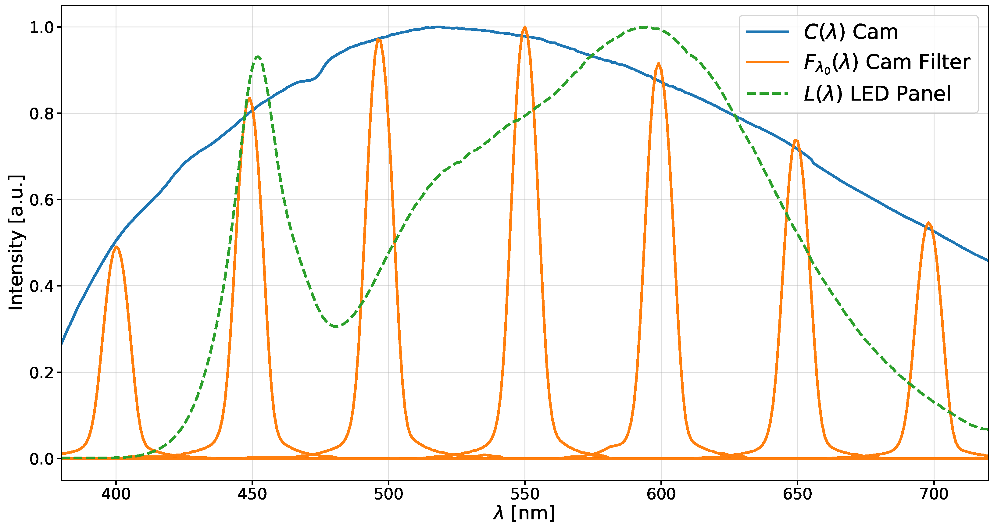
Figure 1. Measured normalised spectral intensity distribution of the light source L ( λ ) (green), the spectral sensitivity of the camera without a filter C ( λ ) (blue), and the spectral sensitivity of the camera combined with the filters F λ 0 ( λ ) (orange), shown as a composite curve. Each individual filter produced a curve with a defining peak at the filter’s centre wavelength, which was then normalised by the maximum value of the 550 n m filter.
Photonics 13 00242 g001
Figure 2. Per-pixel filter transmission loss maps of the six filters used in our measurement setup, with the correction factors displayed on a global colour scale. Additionally, in the title of each map the mean μ and the standard deviation σ is shown. Each pixel in the camera’s FOV is corrected using the corresponding filter employed during measurement to quantify the transmission loss for varying AOI of the incoming light.
Photonics 13 00242 g002
Figure 3. Schematic representation of the experimental setup used in this work. The green spot marks the position of the camera’s aperture (C), defined by the spherical coordinates ( d C , ϑ C , φ C ) . The blue spot marks the position of the centre of the light source (L) with its spherical coordinates ( d l , ϑ l , φ l ) . The green rectangle represents the bandpass filters in the light path towards the detector. The normals of the light source and the camera point towards the origin, which is located at the centre of the top surface of the object.
Photonics 13 00242 g003
Figure 4. Measured optical properties of the grey silicone phantom that was used as both the calibration object and the background for the other recorded objects. The scattering and absorption coefficients (top row) were determined using an integrating-sphere setup, the refractive index (bottom left) with an ellipsometer, and the anisotropy factor (bottom right) via collimated transmission in combination with an integrating sphere.
Photonics 13 00242 g004
Figure 5. Comparison of the middle horizontal (left) and vertical (right) image lines of photographs of the silicone calibration phantom and the simulation of the same scene. Each camera curve (solid lines) and simulation curve (dashed lines) pair per wavelength is displayed in the same colour.
Photonics 13 00242 g005
Figure 6. Recovered reduced scattering and absorption coefficients with the cube geometry for the three silicone materials, yellow (left column), red (middle column), and blue (right column), marked with their respective colours in each plot. The solid black lines represent the reduced scattering and absorption coefficients measured using an integrating-sphere setup, which serve as the reference in the comparison shown below each plot.
Photonics 13 00242 g006
Figure 7. Comparison of photographs of the silicone cube phantoms (second column) and forward renderings with the recovered optical properties (third column). The resulting CIE Δ E 2000 colour-difference maps (fourth column) show the agreement between both scenes. Additionally, the mean Δ E values of the marked regions on the two main faces of the cubes are displayed. The first column shows the middle vertical image lines, marked with red colour in the images, for both the camera images (solid lines) and the simulation (dashed lines) and compares the curves per wavelength.
Photonics 13 00242 g007
Figure 8. Recovered reduced scattering and absorption coefficients from the Einstein geometry for the two silicone materials, yellow (left column) and red (right column), marked with their respective colours in each plot. The solid black lines represent the scattering and absorption coefficients measured using an integrating-sphere setup, which serve as the reference in the comparison shown below each plot.
Photonics 13 00242 g008
Figure 9. Comparison of photographs of the silicone Einstein phantoms (second column) and forward renderings with the recovered optical properties (third column). The resulting CIE Δ E 2000 colour-difference maps (fourth column) show the agreement between both scenes. Additionally, the mean Δ E values of the marked regions are displayed. The first column shows the middle vertical image lines, marked with red colour in the images, for both the camera images (solid lines) and the simulation (dashed lines) and compares the curves for each wavelength.
Photonics 13 00242 g009
Figure 10. Recovered scattering and absorption coefficients using RGB photographs as input, with the cube geometry for the three silicone materials, yellow (left column), red (middle column), and blue (right column), marked with their respective colours in each plot. The solid black lines represent the scattering and absorption coefficients measured using an integrating-sphere setup, which served as the reference in the comparison shown below each plot.
Photonics 13 00242 g010
Figure 11. Comparison of RGB photographs of the silicone cube phantoms (second column) and forward renderings with the recovered optical properties from the RGB fit (third column). The resulting CIE Δ E 2000 colour-difference maps (fourth column) show the agreement between both scenes, where we have focused on the relevant part of the image that contains the cube. The first column shows the middle vertical sRGB channel data, marked in red in the second column, for both the camera images (solid lines) and the simulation (dashed lines).
Photonics 13 00242 g011
Disclaimer/Publisher’s Note: The statements, opinions and data contained in all publications are solely those of the individual author(s) and contributor(s) and not of MDPI and/or the editor(s). MDPI and/or the editor(s) disclaim responsibility for any injury to people or property resulting from any ideas, methods, instructions or products referred to in the content.