Article

Low-Light Image Enhancement with Residual Diffusion Model in Wavelet Domain

College of Intelligence Science and Technology, Natioal University of Defense Technology, Changsha 410073, China
*
Author to whom correspondence should be addressed.
Photonics 2025, 12(9), 832; https://doi.org/10.3390/photonics12090832
Submission received: 30 June 2025 / Revised: 15 August 2025 / Accepted: 20 August 2025 / Published: 22 August 2025

Abstract

In low-light optical imaging, the scarcity of incident photons and the inherent limitations of imaging sensors lead to challenges such as low signal-to-noise ratio, limited dynamic range, and degraded contrast, severely compromising image quality and optical information integrity. To address these challenges, we propose a novel low-light image enhancement technique, LightenResDiff, which combines a residual diffusion model with the discrete wavelet transform. The core innovation of LightenResDiff lies in it accurately restoring the low-frequency components of an image through the residual diffusion model, effectively capturing and reconstructing its fundamental structure, contours, and global features. Additionally, the dual cross-coefficients recovery module (DCRM) is designed to process high-frequency components, enhancing fine details and local contrast. Moreover, the perturbation compensation module (PCM) mitigates noise sources specific to low-light optical environments, such as dark current noise and readout noise, significantly improving overall image fidelity. Experimental results across four widely-used benchmark datasets demonstrate that LightenResDiff outperforms existing methods both qualitatively and quantitatively, surpassing the current state-of-the-art techniques.

1. Introduction

Advancements in digital imaging technology have profoundly transformed sectors such as surveillance, medical diagnostics, and autonomous navigation. However, the physical limitations of imaging sensors, rooted in the fundamental principles of photonics, continue to pose significant challenges, especially in low-light environments. According to the photon transfer theory, when incident light intensity decreases, the number of photons reaching the sensor diminishes, leading to an inevitable decline in the signal-to-noise ratio (SNR). This physical constraint manifests in captured images as amplified noise, reduced contrast, and blurred details, severely degrading image quality and hindering subsequent optical analysis. For instance, in applications like astronomical imaging or night-time surveillance, where photon counts are scarce, the optical sensor’s inability to accurately capture and convert photons into electrical signals becomes a critical bottleneck.
Conventional methods to mitigate these issues, such as increasing ISO or extending exposure, merely address the symptom rather than the underlying optical problem. These adjustments, while enhancing brightness, exacerbate noise induced by the sensor’s dark current and introduce motion blur due to the prolonged photon integration time—both direct consequences of the sensor’s optical characteristics. Traditional image enhancement techniques, including histogram equalization [1,2], Retinex-based algorithms [3,4], and dehazing methods [5], operate at the post-processing stage and often fail to account for the physical noise models inherent in low-light optical imaging. As a result, they frequently produce artifacts or distort the true optical information encoded in the image.
In contrast to traditional methods, deep learning-based approaches excel at maintaining both color accuracy and structural integrity in images. Among these, techniques involving Retinex [6], Generative Adversarial Networks (GANs) [7], and Transformers [8,9] have significantly advanced the field. Deep learning models have demonstrated clear advantages in handling images captured under low-light conditions.
In recent years, denoising diffusion models [10,11,12] have garnered significant attention. These models simulate a diffusion process in which noise is progressively increased over time. By defining a probability distribution over the clean signal at various time steps, diffusion models can effectively leverage the noise reduction process to reconstruct intricate details and textures. Diffusion models have shown remarkable performance in tasks such as super-resolution [13], inpainting [14], and low-light image enhancement (LLIE) [15,16]. Although a small number of studies have applied diffusion models to LLIE, there remains considerable potential for improvement when combined with domain expertise, opening up new possibilities for this task.
Against this backdrop, we introduce an innovative LLIE method that combines the residual diffusion model with the discrete wavelet transform (DWT). This approach effectively improves the quality of image generation. Specifically, the study first applies two-dimensional DWT to decompose low-light images into one low-frequency and three high-frequency coefficients. This process not only reduces spatial dimensions but also preserves the integrity of the information. Following this, the low-frequency coefficients are processed using a residual diffusion model, which involves two sampling steps to generate the low-frequency coefficients of normal-light images. For the three high-frequency coefficients, a dual cross-coefficients recovery module (DRCM) is employed to restore the high-frequency details in normal-light images. Finally, an inverse discrete wavelet transform (IDWT) is used to obtain the normal-light image, and a perturbation compensation module (PCM) is designed to eliminate noise artifacts.
Our main contributions can be summarized as follows:
  • We propose a low-light image enhancement method that utilizes the residual diffusion model in conjunction with the discrete wavelet transform. The residual diffusion model is employed to learn the mapping of low-frequency coefficients during the conversion from low-light to normal-light images.
  • We designed a dual cross-coefficients recovery module to restore high-frequency coefficients. Additionally, we developed a perturbation compensation module to mitigate the impact of noise artifacts.
  • Extensive experimental results on public low-light datasets demonstrate that our method outperforms previous diffusion-based approaches in both distortion metrics and perceptual quality, while also significantly increasing inference speed.

2. Related Work

2.1. Diffusion Models in Images Restoration

With the advent of diffusion models, their applications in visual low-level tasks have become increasingly prevalent. Early diffusion models primarily controlled image generation for restoration by introducing conditions during the diffusion and sampling processes [17,18]. Jiang et al. [19] introduced a conditional diffusion model and propose a novel training strategy involving forward diffusion and reverse denoising during the training phase, which enables the model to maintain content consistency during inference. Wang et al. [20] presented a zero-reference low-light enhancement model that leverages illumination-invariant priors as intermediaries between different lighting conditions and establishes a physical quadruplet prior. A self-supervised diffusion model for hyperspectral image recovery was also developed, operating by inferring parameters of the variational spatial–spectral module during the reverse diffusion process. Liu et al. [21] introduced the residual denoising diffusion model, demonstrating through coefficient transformation that its sampling process aligns with those of standard diffusion models [10], while also proposing a partially path-independent generation process to better understand the inverse process. Zheng et al. [22] introduced a novel selective hourglass mapping method capable of freely converting various distributions into a shared distribution, enabling the model to learn shared information across different distributions.

2.2. Low-Light Image Enhancement

Low-light image enhancement (LLIE) focuses on improving the visual quality of images captured under low-light conditions by enhancing details and colors, while simultaneously reducing noise. Early traditional methods such as NPE [23] and SRIE [24], sought to improve contrast and brightness by estimating the illumination map or using a single-scale Retinex model, but their effectiveness was often limited in complex scenes. Subsequently, Guo et al. [25] introduced a linearization process that decomposed images into reflectance and illumination components, achieving better detail preservation. Wei et al. [6] advanced this approach by integrating deep learning, using multi-scale Convolutional Neural Networks (CNNs) to learn the mapping between low-light and normal-light images, significantly improving both enhancement quality and robustness. Zamir et al. [26] further expanded on this concept by incorporating a multi-level feature fusion mechanism, which enables more refined handling of textures and colors. Guo et al. [27] and Li et al. [28] introduced two end-to-end trainable deep curve estimation methods that do not require paired training data, making them both efficient and practical for real-world applications. Jiang et al. [7] adopted a GAN framework to simulate natural lighting conditions, generating visually pleasing results. Liu et al. [29] proposed a novel, principled framework that integrates knowledge of low-light images and searches for lightweight, prioritized architectures to build effective enhancement networks. Wu et al. [30], inspired by the Retinex model, introduced a deep unfolding network capable of more accurately estimating the brightness distribution of images, thereby enhancing brightness while preserving the original color information and details. Ma et al. [31] introduced a weight-sharing illumination learning process with a self-calibration module, simplifying the complex design of network architecture and achieving enhancement through straightforward operations. Li et al. [32] presented a Fourier domain-based ultra-high-definition image enhancement method and contributed the first ultra-high-definition LLIE dataset. Wang et al. [8] and Zamir et al. [33] designed two transformer-based approaches for image restoration, which can also be applied to low-light enhancement. Wang et al. [34] introduced a transformer method focused on ultra-high-definition low-light enhancement. It adopts a hierarchical structure, which significantly alleviates the computational bottleneck of the ultra-high-definition LLIE task.

3. Preliminaries: Diffusion Models

Diffusion models [10] are probability-based generative models. The core idea involves learning the data distribution and generating new samples through a forward diffusion process (gradually adding noise to the data) and a reverse denoising process (gradually recovering the data from pure noise).

3.1. Forward Diffusion Process

The forward diffusion process is a Markov chain that gradually adds Gaussian noise to the original data I 0 q ( I 0 ) , where q is the distribution of the data. After T steps, the data is transformed into pure Gaussian noise I T N ( 0 , I ) .
The distribution q ( I 1 , , I T I 0 ) for each step and the distribution q ( I t | I t 1 ) at step t are defined as:
q ( I 1 , , I T I 0 ) = t = 1 T q ( I t I t 1 ) ,
q ( I t | I t 1 ) = N ( I t ; 1 β t I t 1 , β t I ) .
Here, { β 1 , β 2 , , β T } is a pre-defined variance schedule, typically set such that 0 < β 1 < β 2 < < β T < 1 , and N denotes a Gaussian distribution.
The noised data I t at step t can be derived as:
I t = α ¯ t I 0 + 1 α ¯ t ϵ t ,
where α t = 1 β t , α ¯ t = s = 1 t α s , and ϵ t N ( 0 , I ) . This means that any step noised data I t in the forward process can be directly obtained from the original data I 0 , avoiding the cumbersome step-by-step noise addition.

3.2. Reverse Denoising Process

The reverse denoising process is the inverse of the forward process. Starting from pure noise I T , the goal is to gradually remove noise and recover a sample I 0 consistent with the original data distribution. Since the true distribution p of the reverse process is difficult to compute directly, diffusion models use a neural network (typically a U-Net) to approximate the distribution p θ .
The distribution p θ ( I 0 : T ) for each step and the distribution p θ ( I t 1 | I t ) at step t 1 can be derived as:
p θ ( I 0 : T ) = p ( I T ) t = 1 T p θ ( I t 1 I t ) ,
p θ ( I t 1 | I t ) = N ( I t 1 ; μ θ ( I t , t ) , Σ θ ( I t , t ) ) .
Here, μ θ and Σ θ are the mean and variance estimated by the neural network, with Σ θ often simplified to a fixed value related to β t . The mean μ θ can be derived as:
μ θ ( I t , t ) = 1 α t I t 1 α t 1 α ¯ t ϵ θ ( I t , t ) .
During training, the diffusion model optimizes the network parameters θ to estimate the noise ϵ θ :
L d i f f = ϵ t ϵ θ ( I t , t ) 2 .
Through this reverse process, the model gradually recovers a sample I 0 consistent with the original data distribution.
The reverse process of diffusion models typically requires T steps (often set to 1000), which can result in long inference times. Song et al. [11] proposed the Denoising Diffusion Implicit Model (DDIM), which breaks the fixed Markov chain constraint, allowing the model to recover high-quality samples in fewer steps (e.g., 50 steps). In this case, the number of steps required for inference is the implicit sampling step S.

4. Method

Figure 1 illustrates the architecture of LightenResDiff. Given a low-light training image, we first perform a 2D discrete wavelet transform (DWT) on it, yielding a set of coefficients. The residual diffusion model [21] is then used to learn the mapping between the most distinctively varying low-frequency coefficients. Following this, the dual cross-coefficients recovery module (DRCM) is applied to transform the remaining three high-frequency coefficients. Finally, a 2D inverse discrete wavelet transform (IDWT) is performed on the enhanced coefficients, and a perturbation compensation module (PCM) is employed to eliminate noise artifacts, producing the final enhanced image.

4.1. Discrete Wavelet Transform

For low-light images, image processing techniques are often employed to enhance visibility. Among these, discrete wavelet transform (DWT) stands out as a powerful and versatile tool, especially in low-light scenarios where preserving image details and structural integrity is paramount.
DWT is a reversible transformation technique that decomposes an image into multiple frequency components without losing information, making it highly suitable for low-light image enhancement. Its ability to separate image data into different frequency bands allows for targeted processing. Unlike some enhancement methods that operate globally and may over-amplify noise or distort contrast, DWT enables localized adjustments in specific frequency ranges, ensuring that fine details and critical features are retained while improving overall visibility. As shown in Equation (8), given an image I, 2D DWT first applies a one-dimensional DWT to each row of the image, obtaining low-frequency and high-frequency components in the horizontal direction. Then, a one-dimensional DWT is applied to each column of the transformed result, yielding four coefficients: low-frequency ( L L ), horizontal high-frequency ( L H ), vertical high-frequency ( H L ), and diagonal high-frequency ( H H ).
{ L L , L H , H L , H H } = DWT ( I ) .
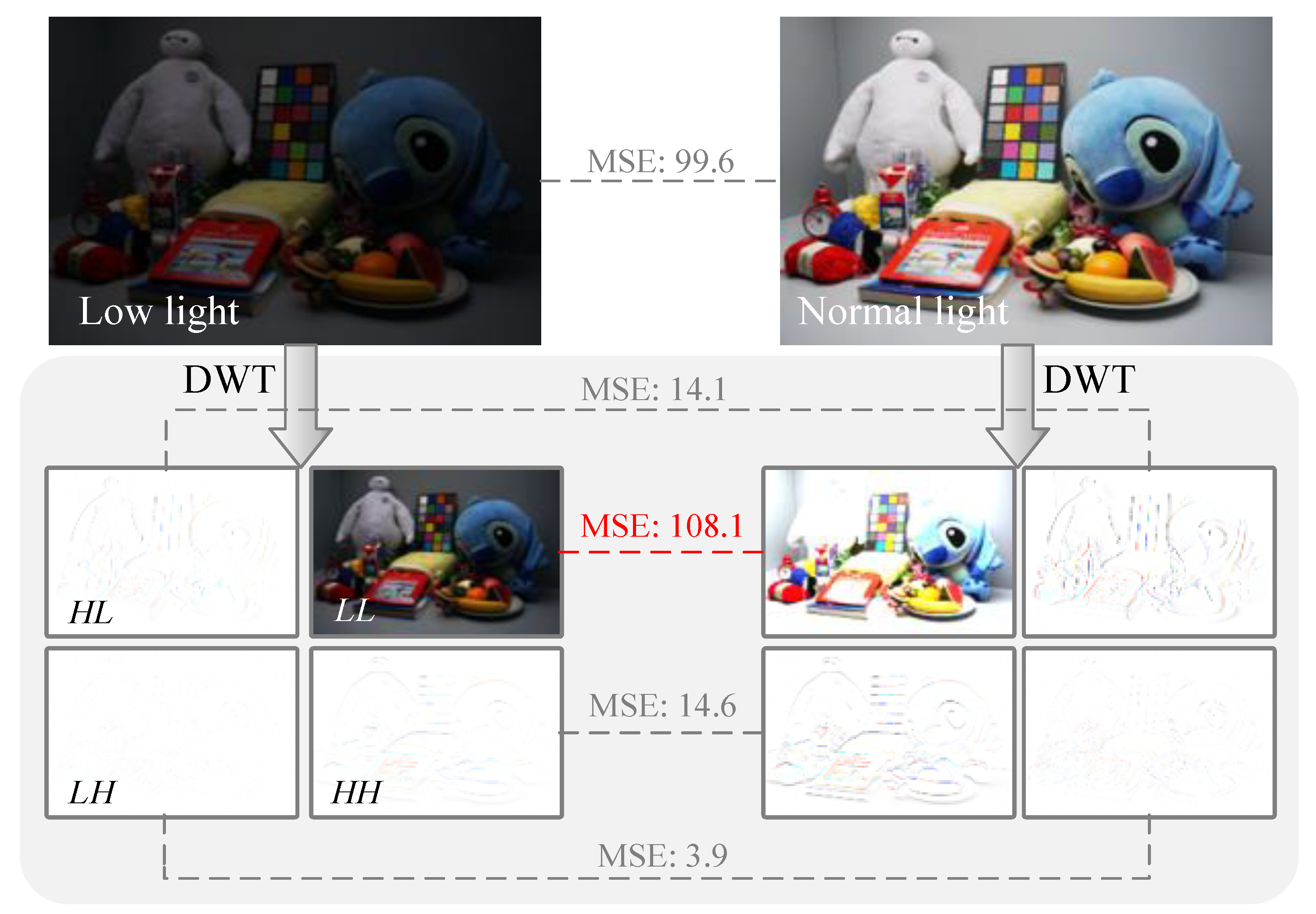
As shown in Figure 2, low-frequency coefficients represent the overall trend of the image, while high-frequency coefficients capture finer details and noise. The most significant difference between low-light and normal-light images is observed in the low-frequency ( L L ) coefficients, with relatively smaller differences in the other three coefficients. Based on this characteristic, a residual diffusion model is specifically employed to train the recovery of L L coefficients, while a lightweight coefficient recovery network is used for the remaining three coefficients. Additionally, the image size is halved after each wavelet transform, which reduces the computational resources required for training and avoids potential degradation in reconstruction quality caused by Variational Autoencoders (VAEs) [35], while achieving encoding efficiency comparable to the VQ-VAE used in latent diffusion models [12].

4.2. Residual Denoising Diffusion Models

The generation process of standard diffusion models starts from random noise, ensuring diversity in the generated results. However, in image restoration tasks like LLIE, the focus shifts to determinism—ensuring the generated data accurately retain the details of the original input. Liu et al. [21] proposed the residual denoising diffusion model, which introduces residuals to make the generated results closer to the target domain, and effectively preserving the input data’s detailed features.

4.2.1. Forward Process

The residual diffusion model employs a dual diffusion mechanism. In the forward diffusion process, noise is added alongside residual components. The distribution q ( I 1 : T | I 0 , I r e s ) for each step and the distribution q ( I t | I t 1 , I r e s ) at step t are defined as:
q ( I 1 : T | I 0 , I r e s ) = t = 1 T q ( I t | I t 1 , I r e s ) ,
q ( I t | I t 1 , I r e s ) = N ( I t ; I t 1 + α t I r e s , β t 2 I ) .
Here, I r e s = I i n I 0 , I 0 represents the target data, and I i n represents the input data. { α 1 , α 2 , , α T } and { β 1 2 , β 2 2 , , β T 2 } are pre-defined coefficient schedules controlling the speed of residual and noise diffusion.
Similarly to the standard diffusion model, the data I t at step t can be directly obtained from the original data I 0 .
I t = I 0 + α ¯ t I r e s + β ¯ t ϵ .
Here, ϵ N ( 0 , I ) , α ¯ t = i = 1 t α i , and β ¯ t = i = 1 t β i 2 . By default, { α 1 , α 2 , , α T } is defined as a sequence that increases uniformly from 0, and α ¯ T = 1 . At step T, the data I T = I i n + β ¯ t ϵ is a noisy input data.

4.2.2. Reverse Process

In the reverse process, the standard diffusion model starts from pure Gaussian noise and gradually reduces noise to generate clear data. In contrast, the residual diffusion model starts from the noisy input data I T = I i n + β ¯ T ϵ . At each step, it not only reduces noise but also removes residuals. If I 0 θ and I r e s θ are known, the reverse generation process can be derived as:
p θ ( I 0 : T ) = p θ ( I T ) t = 1 T p θ ( I t 1 | I t ) ,
p θ ( I t 1 | I t ) = N ( I t 1 ; I t ( α ¯ t α ¯ t 1 ) I r e s θ ( β ¯ t β ¯ t 1 2 σ t 2 ) ϵ θ , σ t 2 I ) ,
where σ t 2 = η β t 2 β ¯ t 1 2 / β ¯ t 2 , and η controls whether the generation process is stochastic ( η = 1 ) or deterministic ( η = 0 ). Setting η = 0 simplifies Equation (13) to:
I t 1 = I t ( α ¯ t α ¯ t 1 ) I r e s θ ( β ¯ t β ¯ t 1 ) ϵ θ ,
I r e s θ or ϵ θ need to be predicted by a neural network (we use a U-Net), and the other one can be derived from Equation (11). We choose to predict I r e s θ , and ϵ θ = ( I t I i n ( α ¯ t 1 ) I r e s θ ) / β ¯ t .
During training, the model’s goal is to optimize the U-Net parameters θ to estimate the residual I r e s θ to be removed at each step:
L r e s = I r e s I r e s θ ( I t , I i n , t ) 2 .
Through this reverse process, the model gradually recovers a sample I 0 consistent with the original data distribution. Similarly to DDIM, the reverse sampling process of the residual diffusion model does not need to follow a fixed Markov chain. Due to the role of the input data, the implicit sampling steps S can be even fewer.

4.3. Dual Cross-Coefficients Recovery Module

For the three high-frequency coefficients of low-light images, vertical, horizontal, and diagonal, we propose a dual cross-coefficients recovery module (DCRM) to establish mappings between these coefficients. This module is designed to enrich the information content of low-light images, thereby aligning it with that of normally lit images.
As shown in Figure 3, the DCRM takes the concatenated three high-frequency coefficients ( L H , H L , H H ) as input. These coefficients first pass through a feature extractor consisting of two sets of Depth-wise Separable Convolution (DSConv) [36] layers and ELU [37] activation layers. Each set includes one DSConv layer, which expands the input from 3 channels to 64 channels, followed by an ELU activation layer. This process results in a 64-channel feature representation for each coefficient. Subsequently, we employ Dual Cross-Attention (DCA) to enrich the details of the H H coefficient using information from the L H and H L coefficients, as illustrated in Figure 4. Simultaneously, two self-attention layers are applied to further capture and refine the characteristics of the L H and H L coefficients. Additionally, drawing from the research of [38], we introduce a progressive spatial dilated Resblock, which facilitates local restoration through dilated convolutions. In this structure, the initial and final convolutional layers focus on extracting local information, while the intermediate dilated convolutional layers capture a broader context by increasing the receptive field. This approach effectively avoids the grid effect that typically results from using a fixed dilation rate. Finally, a DSConv layer reduces the number of channels to complete the reconstruction of the three coefficients.

4.4. Perturbation Compensation Module

Retinex theory suggests that image formation is governed by both the illumination and reflectance components. In mathematical terms, a low-light image I l o w can be expressed as the product of the illumination map L l o w and the reflectance image R, I l o w = L l o w R . A normal-light image I h i g h can also be represented as the product of the illumination map L h i g h and the reflectance image R, I h i g h = L h i g h R . The network model N can be described as achieving: L h i g h = L l o w N . However, in practical scenarios, low-light images are often affected by noise and artifacts [9], leading to the actual situation I ˜ l o w = L l o w + L ¯ l o w R + R ¯ , where L ¯ l o w represents the perturbation of the illumination component and R ¯ represents the perturbation of the reflection component. Therefore, the aforementioned methods, including DWT, the residual diffusion model, and DCRM, can be described in practical testing as a model N and achieve:
I ˜ h i g h = I ˜ l o w N = L l o w R N + L ¯ l o w R + L l o w R ¯ + L ¯ l o w R ¯ N = I h i g h + C .
where C is a perturbation influence term. To compensate for C, we designed a perturbation compensation module (PCM), as shown in Figure 5, which adopts self-attention layers and dilated Resblock from DCRM, pruning unnecessary network structures, and is specifically used for predicting perturbations in a single image. By compensating the network’s predicted results into the IDWT results, we obtain the final enhanced low-light image.

4.5. Training Loss

To train the models discussed earlier, we incorporate three distinct loss functions: the residual loss, the reconstruction loss, and the wavelet loss. It is important to note that the PCM is trained separately, using reconstruction loss (excluding the L2 loss term).
The first loss function, known as the residual loss, is from the residual diffusion model, as shown in Equation (15). And we use L1 loss instead of L2 loss.
L r e s = | I r e s θ I r e s | 1 ,
The second loss function is to guide the training of the DCRM. It is a L2 loss between the predicted normal-light components U ^ high and the ground-truth normal-light components U high in the wavelet domain, where U stands for a union of L H , H L , and H H coefficients.
L d w t = U ^ h i g h U h i g h 2 ,
The final loss function is the reconstruction loss. Generally, the forward process of diffusion models is used for training, while the reverse process is used for inference. Since the residual diffusion model requires only a few implicit sampling steps (set to 2), we can also incorporate the reverse process during training to reconstruct I 0 θ ( L L ^ h i g h ) without significantly increasing the training time. Furthermore, applying IDWT to U ^ h i g h and L L ^ h i g h yields the estimated normal-light image I ^ h i g h . Following prior work [39], we combine L1 loss and MS-SSIM loss to calculate the reconstruction loss and evaluate the effects of MS-SSIM loss in our ablation study.
L r e c = ( L 1 + MS - SSIM ) ( I ^ h i g h , I h i g h ) + L L ^ h i g h L L h i g h 2 ,
In summary, the loss function for the primary network structure is shown below, and we set λ 1 = 1 , λ 2 = 0.1 , and λ 3 = 1 .
L t o t a l = λ 1 L r e s + λ 2 L d w t + λ 3 L r e c .

5. Experiments

5.1. Experimental Settings

Our experiments were conducted on a server equipped with 24 GB of RAM and three NVIDIA RTX 4090 GPUs. We implemented LightenResDiff using Pytorch 2.1.2 [40] and employed two Adam optimizers [41] to train the main architecture network (residual diffusion model, DCRM) and the PCM separately. Both optimizers used an initial learning rate of 8 × 10 5 and momentum parameters set to (0.9, 0.999). During the training phase, we extracted 256 × 256 patches from images for training, with the time step T set to 1000. For the inference phase, the length and width of images were padded to multiples of 64, and the final enhanced results were cropped back to the original size. Meanwhile, the implicit sampling step S was set to 2 for both phases. We set { β 1 2 , β 2 2 , , β T 2 } as a uniformly decreasing sequence terminating at 0, and β ¯ T = 0.1
To validate the low-light enhancement capabilities of our proposed method across different datasets, we selected both paired and unpaired datasets: LOLv1 [6], LOLv2-real [42], LOLv2-syn [42], SID [43], and LSRW [44] as paired datasets and DICM [45], MEF [46], and LIME [25] as unpaired datasets. These datasets were chosen to comprehensively evaluate the effectiveness and generalization ability of our method. For the paired datasets, we evaluated performance using the peak signal-to-noise ratio (PSNR), Structural Similarity Index Measure (SSIM) [47], and Learned Perceptual Image Patch Similarity (LPIPS) [48]. For the unpaired datasets, we conducted evaluations using the Natural Image Quality Evaluator (NIQE) [49] and Blind/Referenceless Image Spatial Quality Evaluator (BRISQUE) [50].
We evaluate the performance of our proposed method against the latest SOTA baselines, including NPE [23], SRIE [24], LIME [25], RetinexNet [6], MIRNet [26], Zero-DCE [27], EnlightenGAN [7], RUAS [29], Uformer [8], Restormer [33], URetinexNet [30], LLformer [34], SCI [31], UHDFour [32], DiffLL [19], RDDM [21], DiffUIR [22], and CoTF [51].

5.2. Comparison with State-of-the-Art Approaches

We validate the effectiveness of our proposed method through extensive experimental evaluations. The experimental results demonstrate that our method achieves leading quantitative performance across all test datasets. Specifically, the data in Table 1 and Table 2 highlight the advantages of our method in terms of distortion metrics. For example, on the LOLv1 test set, the PSNR and SSIM metrics of our method reached 26.49 dB and 0.908, respectively, improving by 0.15 dB and 0.005 over the second-best methods, DiffLL and DiffUIR. On the LOLv2-real test dataset, our method’s SSIM value of 0.897 improved by 0.021 compared to DiffLL. On the LOLv2-syn test set, our method’s PSNR and SSIM metrics were 25.68 dB and 0.938, respectively, which were 0.92 dB and 0.002 higher than those of CoTF. On the SID and LSRW test sets, our method achieved PSNR values of 24.83 dB and 21.12 dB and SSIM values of 0.764 and 0.636, respectively. This represents an improvement of 0.12 dB and 1.34 dB in PSNR and 0.014 and 0.029 in SSIM over the comparison methods.
In terms of the perceptual metric LPIPS, our method excels, particularly where transformer-based and other diffusion-based methods underperform. It demonstrated the best visual quality restoration across LOLv1, LOLv2-real, LOLv2-syn, and SID, outperforming the next best method by 0.004, 0.045, 0.004, and 0.031. To further validate the effectiveness and generalization ability of our method, we conducted a detailed comparison with existing competitive methods across three unpaired datasets. We used two no-reference perceptual metrics, NIQE and BRISQUE, to evaluate the visual quality of enhanced images, with lower scores indicating higher visual quality. As shown in Table 3, our method achieved the best NIQE scores on the DICM and LIME datasets, with scores of 3.829 and 3.866 respectively. For BRISQUE scores, our method achieved the best results on the MEF, LIME, and NPE datasets, with scores of 22.494, 18.049, and 13.841 respectively. These quantitative analysis results not only confirm the excellent image enhancement performance of our method on known datasets but also demonstrate its ability to provide high-quality enhancement in unseen real-world scenarios. This suggests that our method holds significant advantages and broad application potential in solving practical LLIE problems.
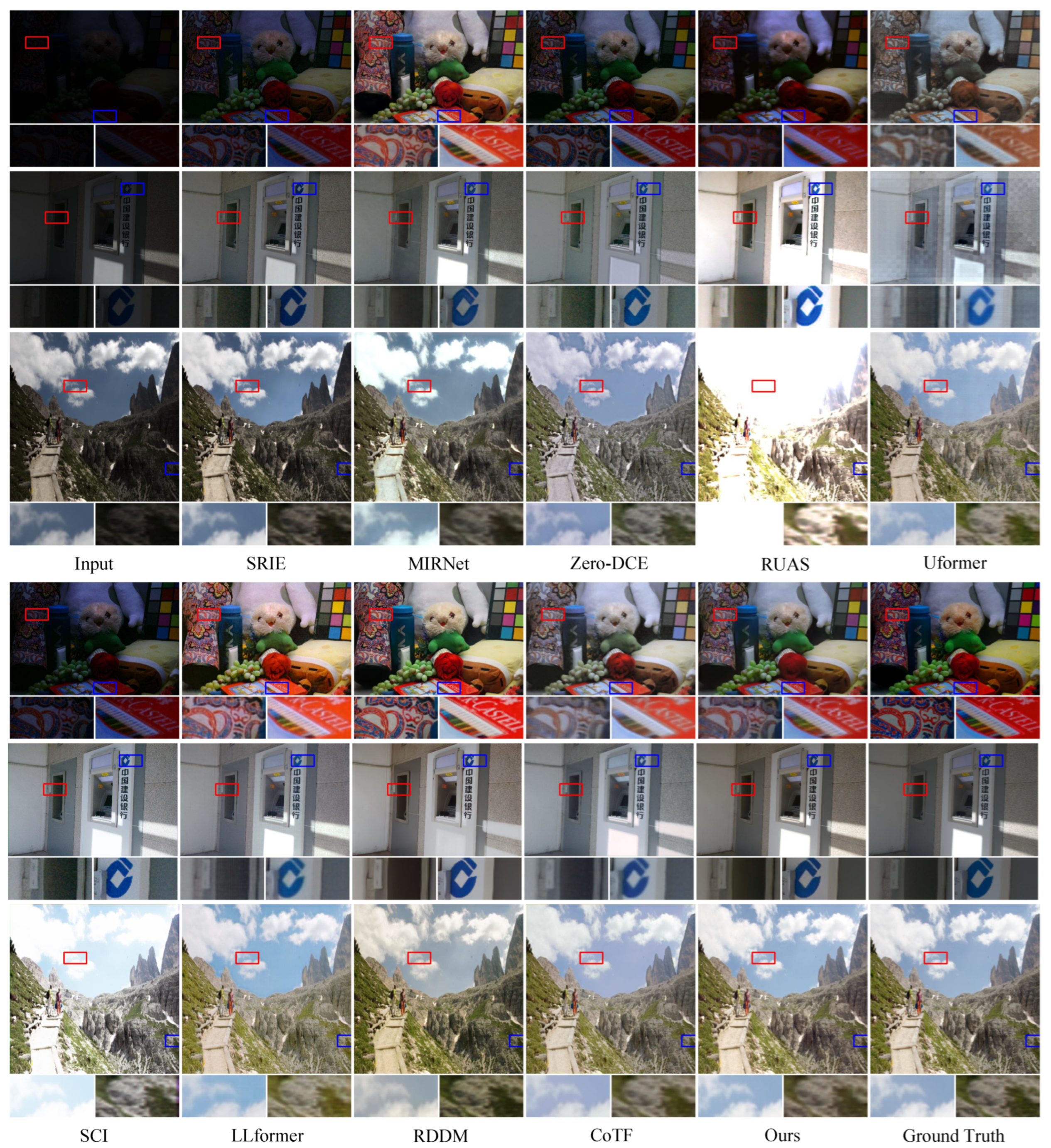
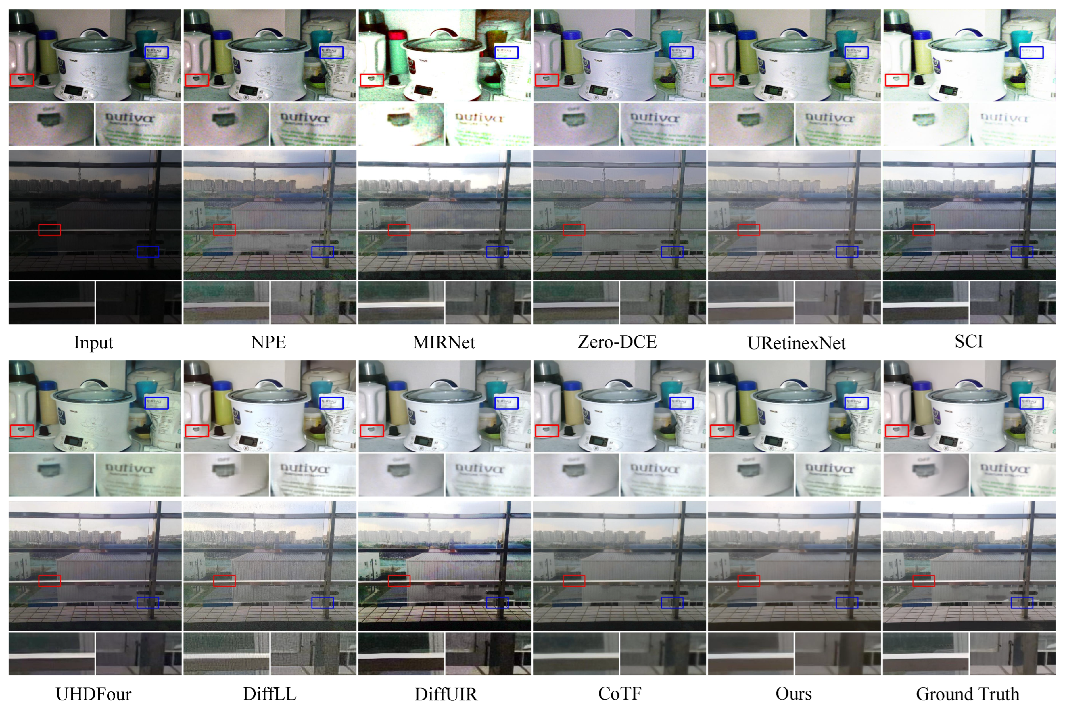
To more intuitively showcase the advantages of our method, we conducted qualitative comparisons on both paired and unpaired datasets. Figure 6 and Figure 7 present image samples from the LOLv1, LOLv2-real, LOLv2-syn, SID, and LSRW test sets, comparing the performance of our method against current SOTA approaches.
Figure 6 demonstrates that RUAS struggles with accurately capturing brightness on both the LOLv1, LOLv2-real, and LOLv2-syn datasets. Specifically, on the LOLv1 dataset, RUAS appears relatively dim, whereas on the LOLv2-real dataset, despite an increase in contrast, it still exhibits overexposure issues. SRIE, Zero-DCE, RUAS, MIRNet, and SCI perform poorly in recovering the original image brightness. LLformer has limited effectiveness in noise reduction, causing text on books and bank logos to appear blurry. Images enhanced by RDDM and CoTF tend to have dull colors, with the overall picture appearing overly white. In contrast, our proposed method accurately restores the original colors and lighting conditions, showcasing the best overall performance. Figure 7 further highlights the restoration issues caused by other methods, such as noise and color distortion, when applied to the SID and LSRW datasets. For instance, NPE, MIRNet, Zero-DCE, and URetinexNet retain noticeable noise in certain image regions, especially around the base of the kettle. When the brightness of a low-light image is not low enough, SCI trends to overexpose the image. UHDFour, DiffLL, DiffUIR, and CoTF show significant color deviations in specific areas, such as bags appearing unnaturally green or washed out. In contrast, our method excels in enhancing both global and local contrast, recovering fine details, suppressing noise, and ensuring high-quality visual enhancement across various scenarios. We also provide a visual comparison of our method against competing methods on unpaired datasets in Figure 8. On the DICM dataset, our method avoids overexposure issues compared to SCI. On the LIME dataset, our method eliminates the appearance of a purple tint. Finally, on the MEF and NPE datasets, our method better preserves the natural green colors of vegetation compared to UHDFour and RDDM. These results demonstrate that our method generalizes effectively to unseen scenes.
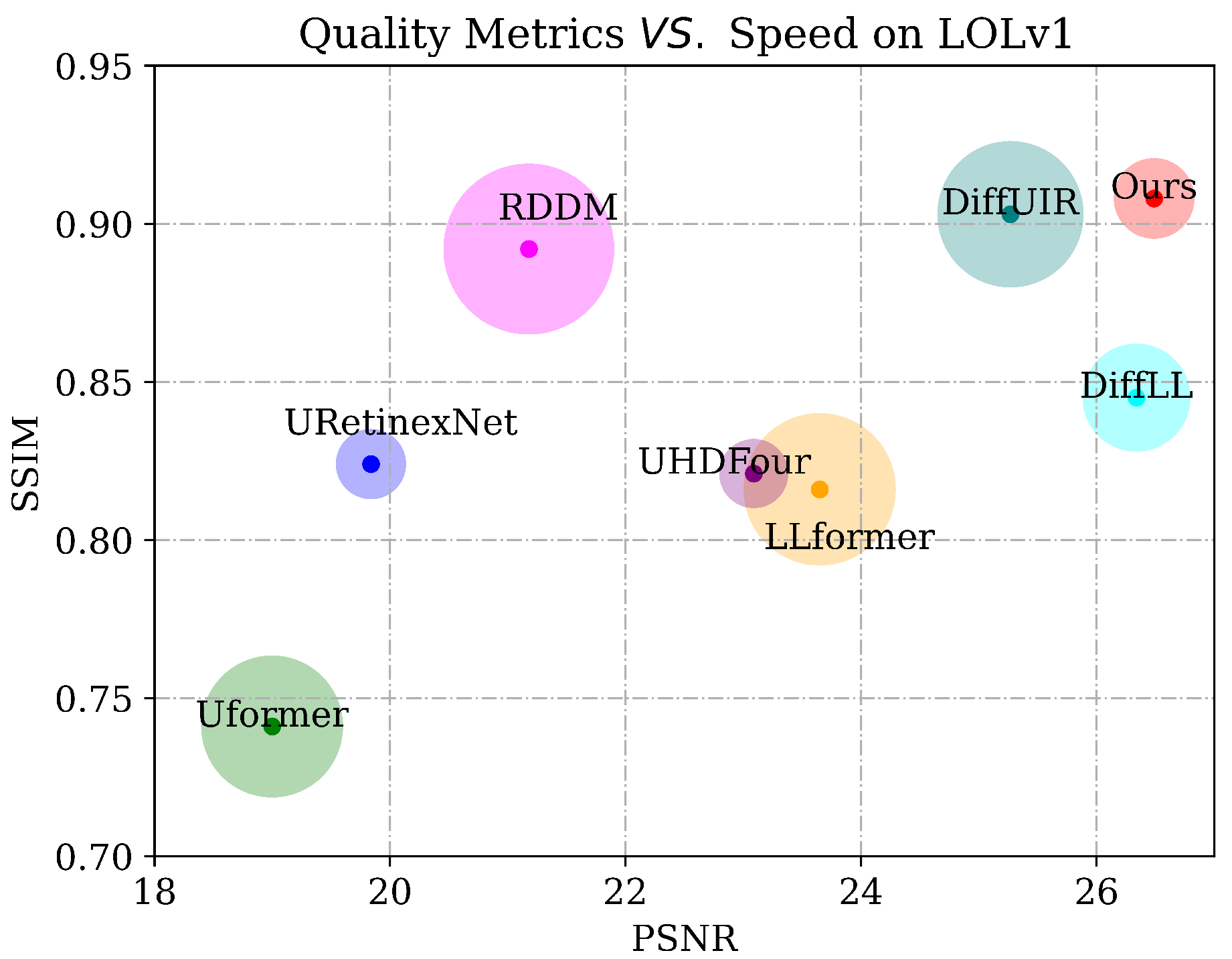
Besides improving visual quality, efficiency plays a key role in image restoration tasks. To assess this, we compared the number of parameters, average inference time, and GPU memory consumption of our method with competing methods on the LOLv1 test set. The tests were conducted using 600 × 400 resolution images, with all experiments performed on the same machine equipped with an NVIDIA RTX 4090 GPU and a batch size of 1. Table 4 shows that our method has a moderate number of parameters. However, it strikes an excellent balance between performance and efficiency, with an average processing time of 0.087 s per image and GPU memory usage of 1.391 GB, both the best among the compared methods. Figure 9 intuitively shows the comparison between metrics and inference time. Due to the two-step sampling and image reduction achieved through wavelet transform, our method reduces the inference time by approximately 50% compared to previous diffusion model-based restoration methods while slightly decreasing computational resource requirements.

5.3. Low-Light Object Detection

To assess the influence of different image enhancement techniques on high-level visual tasks, we performed low-light object detection experiments using the ExDark dataset [52]. The ExDark dataset consists of 7363 underexposed images, each annotated with bounding boxes for 12 object categories. We excluded images without three channels, resulting in 5841 images for training and 1422 for testing. For object detection, we employed YOLOv11 [53], and trained it from scratch. Various low-light enhancement algorithms were used as fixed-parameter preprocessing steps. Figure 10a presents the Precision–Recall (P-R) curves for all categories, while Table 5 lists the Average Precision (AP@50:95) scores for each category. Our method achieved the highest mean Average Precision (mAP@50:95) of 0.410, outperforming the most recent supervised method, LLformer, by 0.01 and the most recent unsupervised method, SCI, by 0.012. Notably, our method performed best in five specific categories: boats, bottles, buses, motorcycles, and tables. Figure 10b provides a visual comparison of detection results in low-light conditions (left) versus after LightenResDiff enhancement (right). In the original low-light scenes, detectors tend to miss some boats or make inaccurate predictions due to underexposure. However, when using images enhanced by our LightenResDiff method, the detector operates more reliably, accurately predicting well-placed bounding boxes that cover all boats. This demonstrates the effectiveness of our method in enhancing the performance of high-level visual tasks.

5.4. Ablation Study

We conduct a series of ablation studies to evaluate the effectiveness of several key components of our method. All ablation experiments are performed using the LOLv1 dataset [6]. As shown in Table 6, our default setting is in bold.

5.4.1. Image Preprocessing

We applied the DWT to the training images before training commenced. Furthermore, we continued to perform DWT on the decomposed low-frequency coefficients. To evaluate the impact of DWT times, we compared the performance of our proposed method against two preprocessing approaches: no preprocessing, and applying the wavelet transform twice. The results are shown in Table 6. Our experiments demonstrate that the wavelet transform is an effective preprocessing method. Regardless of whether the wavelet transform is applied once or twice, our method outperforms no preprocessing in both cases. By default, we apply the wavelet transform once, though for generating ultra-high-definition images, the number of iterations can be adjusted to two.

5.4.2. Loss Function

As shown in Section 4.5, our loss function consists of three distinct components. To evaluate the effectiveness of each part, we conducted experiments by individually removing each component from the default configuration. The results in Table 6 reveal that removing the residual loss L r e s led to a decline in visual quality metrics, but not to a catastrophic extent. This is attributed to the fact that the reconstruction loss L r e c also plays a role in guiding the prediction of residuals and the generation of images by the residual diffusion model. The wavelet loss L d w t is designed to guide the training of the DCRM and to enhance the details in image reconstruction; hence, its removal negatively impacts performance. Among the components, the reconstruction loss is the most effective. Upon introducing the reconstruction loss, we observed an improvement of 1.36 dB in PSNR, an increase of 0.026 in SSIM, and a reduction of 0.032 in LPIPS. Furthermore, replacing the L1 loss in reconstruction loss with L1 + MS-SSIM loss also enhances the generation quality. The incorporation of MS-SSIM loss positively contributes to the visual quality of denoised images, thereby enhancing the overall performance.

5.4.3. Module Architecture

To validate the effectiveness of our designed DCRM and PCM, we used a residual diffusion model for recovering low-frequency coefficients as the baseline. We then augmented this baseline model by adding the DCRM and PCM modules. Specifically, we constructed two versions of DCRM and two versions of PCM. DCRM v 1 is a version without self-attention layers and dual cross-attention layers [54], where each coefficient focuses solely on its own features. DCRM v 2 is our default version, which leverages DCA layers to enhance the HH coefficients, as the L H and H L coefficients contain diagonal high-frequency components, and uses self-attention layers to capture long-range dependencies. PCM v 1 only uses one set of dilated Resblock, whereas PCM v 2 , the default version, employs two sets of self-attention layer and dilated Resblock. As shown in Table 6, the addition and iteration of DCRM and PCM significantly improve the generation quality.

5.4.4. Noise Factor and Sampling Steps

In the residual diffusion model, { β 1 2 , β 2 2 , , β T 2 } controls the speed of noise diffusion, which we refer to as the noise factor. To assess the impact of different noise factors and implicit sampling steps S on model performance, we conducted experiments evaluating the model’s behavior under varying noise factors and sampling steps. For { β 1 2 , β 2 2 , , β T 2 } , we still maintain a uniformly decreasing schedule, but modify the values of β ¯ T . A visual comparison is shown in Figure 11, and the quantitative scores are presented in Table 6. It was observed that when β ¯ T is set to 1, the model’s performance drops significantly; this is because the increased initial noise injection enhances generation diversity. As the number of sampling steps increases, the time required for model training and sample generation increases rapidly. However, while the quality of image generation improves initially, it eventually plateaus. Therefore, for the number of sampling steps, we chose a balanced middle value of 2.

6. Discussion

This study proposes a novel low-light image enhancement method that combines a residual diffusion model with discrete wavelet transform (DWT), achieving significant improvements in image quality, inference speed, and robustness against noise artifacts.
Low-light image enhancement has long faced two key challenges: avoiding noise amplification while preserving fine details, and balancing generation quality with computational efficiency. Previous diffusion-based methods [15,55], despite their strong generation capabilities, often suffer from slow inference speeds due to iterative sampling. In contrast, our method addresses these limitations through a dual-focus strategy: utilizing DWT to separate low-frequency structures and high-frequency details, and designing task-specific modules for each component.
Extensive experiments on multiple datasets validate the generalization ability of our method. On the widely used LOLv1 dataset, our method maintains a peak signal-to-noise ratio of 26.49 dB, outperforming both diffusion-based [19,21,22] and non-diffusion [51] methods. This indicates that frequency-domain decomposition and dedicated modules exhibit strong robustness to varying degrees of illumination degradation.
A breakthrough aspect of our method lies in its improved inference speed. Most diffusion-based low-light image enhancement models require 50–100 sampling steps [16], whereas our residual diffusion model completes low-frequency generation in only two steps. Importantly, this efficiency improvement is not achieved at the expense of quality. This balance between speed and quality is crucial for practical applications such as surveillance and night photography, where latency is a key constraint.
Despite these advantages, our method has limitations. For instance, the choice of DWT decomposition levels may affect model performance; the current level setting is determined based on experimental experience, and adaptive level selection strategies could be further explored in the future. Additionally, the model’s performance in processing extremely low-light images (e.g., where light intensity is close to darkness) still has room for improvement, and optimization by incorporating more advanced noise modeling methods could be considered. Our future work will consider applying the proposed DRCM and PCM to general image restoration tasks.

7. Conclusions

In conclusion, LightenResDiff combines the residual diffusion model, DCRM, and wavelet transforms to achieve efficient image enhancement and restore the information that is otherwise lost due to low photon counts. The integration of three distinct loss functions and a PCM further enhances perceptual quality. Experimental results demonstrate that LightenResDiff excels in perceptual metrics, producing enhanced images that align closely with human perception. This study employs deep learning algorithms to compensate for optical limitations in low-light imaging, demonstrating the enormous potential of diffusion models in the fields of photonics and optical sensing. Future work will explore the development of a more general image enhancement method.

Author Contributions

Conceptualization, B.D. and B.S.; methodology, B.D.; software, B.D.; validation, B.D., D.B. and Y.W.; formal analysis, B.D.; investigation, B.D. and D.B.; resources, B.D. and D.B.; data curation, B.D. and Y.W.; writing—original draft preparation, B.D., D.B., B.S. and X.S.; writing—review and editing, B.D., D.B., B.S. and W.J.; visualization, B.D.; supervision, B.S.; project administration, H.Q. and X.S.; funding acquisition, B.S. and W.J. All authors have read and agreed to the published version of the manuscript.

Funding

This research received no external funding.

Institutional Review Board Statement

Not applicable.

Informed Consent Statement

Not applicable.

Data Availability Statement

The original contributions presented in the study are included in the article; further inquiries can be directed to the corresponding author.

Conflicts of Interest

The authors declare no conflicts of interest.

References

  1. Singh, K.; Kapoor, R.; Sinha, S.K. Enhancement of low exposure images via recursive histogram equalization algorithms. Optik 2015, 126, 2619–2625. [Google Scholar] [CrossRef]
  2. Wang, Q.; Ward, R.K. Fast image/video contrast enhancement based on weighted thresholded histogram equalization. IEEE Trans. Consum. Electron. 2007, 53, 757–764. [Google Scholar] [CrossRef]
  3. Rahman, Z.U.; Jobson, D.J.; Woodell, G.A. Multi-scale retinex for color image enhancement. In Proceedings of the 3rd IEEE International Conference on Image Processing, Lausanne, Switzerland, 19 September 1996; Volume 3, pp. 1003–1006. [Google Scholar]
  4. Cai, R.; Chen, Z. Brain-like retinex: A biologically plausible retinex algorithm for low light image enhancement. Pattern Recognit. 2023, 136, 109195. [Google Scholar] [CrossRef]
  5. Tang, Q.; Yang, J.; He, X.; Jia, W.; Zhang, Q.; Liu, H. Nighttime image dehazing based on Retinex and dark channel prior using Taylor series expansion. Comput. Vis. Image Underst. 2021, 202, 103086. [Google Scholar] [CrossRef]
  6. Wei, C.; Wang, W.; Yang, W.; Liu, J. Deep retinex decomposition for low-light enhancement. arXiv 2018, arXiv:1808.04560. [Google Scholar] [CrossRef]
  7. Jiang, Y.; Gong, X.; Liu, D.; Cheng, Y.; Wang, Z. EnlightenGAN: Deep Light Enhancement Without Paired Supervision. IEEE Trans. Image Process. 2021, 30, 2340–2349. [Google Scholar] [CrossRef]
  8. Wang, Z.; Cun, X.; Bao, J.; Zhou, W.; Liu, J.; Li, H. Uformer: A general u-shaped transformer for image restoration. In Proceedings of the IEEE/CVF Conference on Computer Vision and Pattern Recognition, New Orleans, LO, USA, 18–24 June 2022; pp. 17683–17693. [Google Scholar]
  9. Cai, Y.; Bian, H.; Lin, J.; Wang, H.; Timofte, R.; Zhang, Y. Retinexformer: One-stage retinex-based transformer for low-light image enhancement. In Proceedings of the IEEE/CVF International Conference on Computer Vision, Paris, France, 1–6 October 2023; pp. 12504–12513. [Google Scholar]
  10. Ho, J.; Jain, A.; Abbeel, P. Denoising diffusion probabilistic models. Adv. Neural Inf. Process. Syst. 2020, 33, 6840–6851. [Google Scholar]
  11. Song, J.; Meng, C.; Ermon, S. Denoising diffusion implicit models. arXiv 2020, arXiv:2010.02502. [Google Scholar]
  12. Rombach, R.; Blattmann, A.; Lorenz, D.; Esser, P.; Ommer, B. High-resolution image synthesis with latent diffusion models. In Proceedings of the IEEE/CVF Conference on Computer Vision and Pattern Recognition, New Orleans, LO, USA, 18–24 June 2022; pp. 10684–10695. [Google Scholar]
  13. Saharia, C.; Ho, J.; Chan, W.; Salimans, T.; Fleet, D.J.; Norouzi, M. Image super-resolution via iterative refinement. IEEE Trans. Pattern Anal. Mach. Intell. 2022, 45, 4713–4726. [Google Scholar] [CrossRef] [PubMed]
  14. Saharia, C.; Chan, W.; Chang, H.; Lee, C.; Ho, J.; Salimans, T.; Fleet, D.; Norouzi, M. Palette: Image-to-image diffusion models. In Proceedings of the ACM SIGGRAPH 2022 Conference Proceedings, Vancouver, BC, Canada, 8–11 August 2022; pp. 1–10. [Google Scholar]
  15. Yi, X.; Xu, H.; Zhang, H.; Tang, L.; Ma, J. Diff-retinex: Rethinking low-light image enhancement with a generative diffusion model. In Proceedings of the IEEE/CVF International Conference on Computer Vision, Paris, France, 1–6 October 2023; pp. 12302–12311. [Google Scholar]
  16. Yang, S.; Zhang, X.; Wang, Y.; Yu, J.; Wang, Y.; Zhang, J. Difflle: Diffusion-guided domain calibration for unsupervised low-light image enhancement. arXiv 2023, arXiv:2308.09279. [Google Scholar]
  17. Dhariwal, P.; Nichol, A. Diffusion models beat gans on image synthesis. Adv. Neural Inf. Process. Syst. 2021, 34, 8780–8794. [Google Scholar]
  18. Ho, J.; Salimans, T. Classifier-free diffusion guidance. arXiv 2022, arXiv:2207.12598. [Google Scholar] [CrossRef]
  19. Jiang, H.; Luo, A.; Fan, H.; Han, S.; Liu, S. Low-light image enhancement with wavelet-based diffusion models. ACM Trans. Graph. (TOG) 2023, 42, 1–14. [Google Scholar] [CrossRef]
  20. Wang, W.; Yang, H.; Fu, J.; Liu, J. Zero-reference low-light enhancement via physical quadruple priors. In Proceedings of the IEEE/CVF Conference on Computer Vision and Pattern Recognition, Seattle, WA, USA, 16–22 June 2024; pp. 26057–26066. [Google Scholar]
  21. Liu, J.; Wang, Q.; Fan, H.; Wang, Y.; Tang, Y.; Qu, L. Residual denoising diffusion models. In Proceedings of the IEEE/CVF Conference on Computer Vision and Pattern Recognition, Seattle, WA, USA, 16–22 June 2024; pp. 2773–2783. [Google Scholar]
  22. Zheng, D.; Wu, X.M.; Yang, S.; Zhang, J.; Hu, J.F.; Zheng, W.S. Selective hourglass mapping for universal image restoration based on diffusion model. In Proceedings of the Proceedings of the IEEE/CVF Conference on Computer Vision and Pattern Recognition, Seattle, WA, USA, 16–22 June 2024; pp. 25445–25455. [Google Scholar]
  23. Wang, S.; Zheng, J.; Hu, H.M.; Li, B. Naturalness preserved enhancement algorithm for non-uniform illumination images. IEEE Trans. Image Process. 2013, 22, 3538–3548. [Google Scholar] [CrossRef] [PubMed]
  24. Fu, X.; Zeng, D.; Huang, Y.; Zhang, X.P.; Ding, X. A weighted variational model for simultaneous reflectance and illumination estimation. In Proceedings of the IEEE Conference on Computer Vision and Pattern Recognition, Las Vegas, NV, USA, 27–30 June 2016; pp. 2782–2790. [Google Scholar]
  25. Guo, X.; Li, Y.; Ling, H. LIME: Low-light image enhancement via illumination map estimation. IEEE Trans. Image Process. 2016, 26, 982–993. [Google Scholar] [CrossRef]
  26. Zamir, S.W.; Arora, A.; Khan, S.; Hayat, M.; Khan, F.S.; Yang, M.H.; Shao, L. Learning enriched features for real image restoration and enhancement. In Proceedings of the Computer Vision–ECCV 2020: 16th European Conference, Glasgow, UK, 23–28 August 2020; Springer: Berlin/Heidelberg, Germany, 2020. Proceedings, Part XXV 16. pp. 492–511. [Google Scholar]
  27. Guo, C.; Li, C.; Guo, J.; Loy, C.C.; Hou, J.; Kwong, S.; Cong, R. Zero-reference deep curve estimation for low-light image enhancement. In Proceedings of the IEEE/CVF Conference on Computer Vision and Pattern Recognition, online, 16–18 June 2020; pp. 1780–1789. [Google Scholar]
  28. Li, C.; Guo, C.; Loy, C.C. Learning to enhance low-light image via zero-reference deep curve estimation. IEEE Trans. Pattern Anal. Mach. Intell. 2021, 44, 4225–4238. [Google Scholar] [CrossRef]
  29. Liu, R.; Ma, L.; Zhang, J.; Fan, X.; Luo, Z. Retinex-inspired unrolling with cooperative prior architecture search for low-light image enhancement. In Proceedings of the IEEE/CVF Conference on Computer Vision and Pattern Recognition, Nashville, TN, USA, 20–25 June 2021; pp. 10561–10570. [Google Scholar]
  30. Wu, W.; Weng, J.; Zhang, P.; Wang, X.; Yang, W.; Jiang, J. Uretinex-net: Retinex-based deep unfolding network for low-light image enhancement. In Proceedings of the IEEE/CVF Conference on Computer Vision and Pattern Recognition, New Orleans, LO, USA, 18–24 June 2022; pp. 5901–5910. [Google Scholar]
  31. Ma, L.; Ma, T.; Liu, R.; Fan, X.; Luo, Z. Toward fast, flexible, and robust low-light image enhancement. In Proceedings of the IEEE/CVF Conference on Computer Vision and Pattern Recognition, New Orleans, LO, USA, 18–24 June 2022; pp. 5637–5646. [Google Scholar]
  32. Li, C.; Guo, C.L.; Zhou, M.; Liang, Z.; Zhou, S.; Feng, R.; Loy, C.C. Embedding fourier for ultra-high-definition low-light image enhancement. arXiv 2023, arXiv:2302.11831. [Google Scholar]
  33. Zamir, S.W.; Arora, A.; Khan, S.; Hayat, M.; Khan, F.S.; Yang, M.H. Restormer: Efficient transformer for high-resolution image restoration. In Proceedings of the IEEE/CVF Conference on Computer Vision and Pattern Recognition, New Orleans, LO, USA, 18–24 June 2022; pp. 5728–5739. [Google Scholar]
  34. Wang, T.; Zhang, K.; Shen, T.; Luo, W.; Stenger, B.; Lu, T. Ultra-high-definition low-light image enhancement: A benchmark and transformer-based method. In Proceedings of the AAAI Conference on Artificial Intelligence, Washington, DC, USA, 7–14 February 2023; Volume 37, pp. 2654–2662. [Google Scholar]
  35. Van Den Oord, A.; Vinyals, O.; Kavukcuoglu, K. Neural discrete representation learning. In Proceedings of the 31st International Conference on Neural Information Processing Systems, Long Beach, CA, USA, 4–9 December 2017. [Google Scholar]
  36. Chollet, F. Xception: Deep learning with depthwise separable convolutions. In Proceedings of the IEEE Conference on Computer Vision and Pattern Recognition, Honolulu, HI, USA, 21–26 July 2017; pp. 1251–1258. [Google Scholar]
  37. Clevert, D.A.; Unterthiner, T.; Hochreiter, S. Fast and accurate deep network learning by exponential linear units (elus). arXiv 2015, arXiv:1511.07289. [Google Scholar]
  38. Hai, J.; Yang, R.; Yu, Y.; Han, S. Combining spatial and frequency information for image deblurring. IEEE Signal Process. Lett. 2022, 29, 1679–1683. [Google Scholar] [CrossRef]
  39. Zhao, H.; Gallo, O.; Frosio, I.; Kautz, J. Loss functions for image restoration with neural networks. IEEE Trans. Comput. Imaging 2016, 3, 47–57. [Google Scholar] [CrossRef]
  40. Paszke, A. Pytorch: An imperative style, high-performance deep learning library. arXiv 2019, arXiv:1912.01703. [Google Scholar]
  41. Kingma, D.P.; Ba, J. Adam: A method for stochastic optimization. arXiv 2014, arXiv:1412.6980. [Google Scholar]
  42. Yang, W.; Wang, S.; Fang, Y.; Wang, Y.; Liu, J. From fidelity to perceptual quality: A semi-supervised approach for low-light image enhancement. In Proceedings of the IEEE/CVF Conference on Computer Vision and Pattern Recognition, Online, 14–19 June 2020; pp. 3063–3072. [Google Scholar]
  43. Chen, C.; Chen, Q.; Xu, J.; Koltun, V. Learning to see in the dark. In Proceedings of the IEEE Conference on Computer Vision and Pattern Recognition, Salt Lake City, UT, USA, 18–22 June 2018; pp. 3291–3300. [Google Scholar]
  44. Hai, J.; Xuan, Z.; Yang, R.; Hao, Y.; Zou, F.; Lin, F.; Han, S. R2rnet: Low-light image enhancement via real-low to real-normal network. J. Vis. Commun. Image Represent. 2023, 90, 103712. [Google Scholar] [CrossRef]
  45. Lee, C.; Lee, C.; Kim, C.S. Contrast enhancement based on layered difference representation of 2D histograms. IEEE Trans. Image Process. 2013, 22, 5372–5384. [Google Scholar] [CrossRef]
  46. Lee, C.; Lee, C.; Lee, Y.Y.; Kim, C.S. Power-constrained contrast enhancement for emissive displays based on histogram equalization. IEEE Trans. Image Process. 2011, 21, 80–93. [Google Scholar] [CrossRef] [PubMed]
  47. Wang, Z.; Bovik, A.C.; Sheikh, H.R.; Simoncelli, E.P. Image quality assessment: From error visibility to structural similarity. IEEE Trans. Image Process. 2004, 13, 600–612. [Google Scholar] [CrossRef]
  48. Zhang, R.; Isola, P.; Efros, A.A.; Shechtman, E.; Wang, O. The unreasonable effectiveness of deep features as a perceptual metric. In Proceedings of the IEEE Conference on Computer Vision and Pattern Recognition, Salt Lake City, UT, USA, 18–22 June 2018; pp. 586–595. [Google Scholar]
  49. Mittal, A.; Soundararajan, R.; Bovik, A.C. Making a “completely blind” image quality analyzer. IEEE Signal Process. Lett. 2012, 20, 209–212. [Google Scholar] [CrossRef]
  50. Mittal, A.; Moorthy, A.K.; Bovik, A.C. No-reference image quality assessment in the spatial domain. IEEE Trans. Image Process. 2012, 21, 4695–4708. [Google Scholar] [CrossRef]
  51. Li, Z.; Zhang, F.; Cao, M.; Zhang, J.; Shao, Y.; Wang, Y.; Sang, N. Real-time exposure correction via collaborative transformations and adaptive sampling. In Proceedings of the of the IEEE/CVF Conference on Computer Vision and Pattern Recognition, Seattle, WA, USA, 17–21 June 2024; pp. 2984–2994. [Google Scholar]
  52. Loh, Y.P.; Chan, C.S. Getting to know low-light images with the exclusively dark dataset. Comput. Vis. Image Underst. 2019, 178, 30–42. [Google Scholar] [CrossRef]
  53. Khanam, R.; Hussain, M. Yolov11: An overview of the key architectural enhancements. arXiv 2024, arXiv:2410.17725. [Google Scholar] [CrossRef]
  54. Hou, R.; Chang, H.; Ma, B.; Shan, S.; Chen, X. Cross attention network for few-shot classification. In Proceedings of the 33rd International Conference on Neural Information Processing Systems, Vancouver, BC, Canada, 8–14 December 2019. [Google Scholar]
  55. Yi, X.; Xu, H.; Zhang, H.; Tang, L.; Ma, J. Diff-Retinex++: Retinex-Driven Reinforced Diffusion Model for Low-Light Image Enhancement. IEEE Trans. Pattern Anal. Mach. Intell. 2025, 47, 6823–6841. [Google Scholar] [CrossRef] [PubMed]
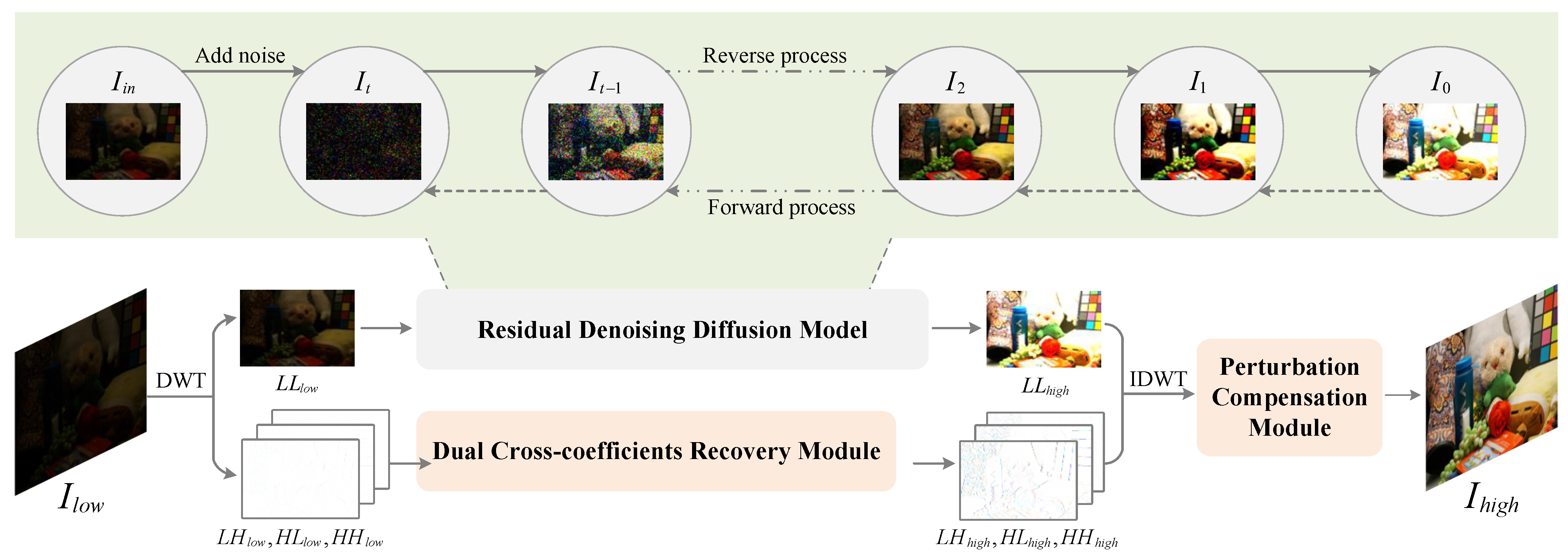
Figure 1. The overall architecture of our proposed LightenResDiff.
Photonics 12 00832 g001
Figure 2. Mean Squared Error (MSE) and visual gap between the four components of low-light and normal-light images after DWT.
Photonics 12 00832 g002
Figure 3. The architecture of our proposed dual DCRM. DSConv stands for depth-wise separable convolution, SA stands for self-attention, and DCA stands for dual cross-attention.
Photonics 12 00832 g003
Figure 4. The architecture of DCA.
Photonics 12 00832 g004
Figure 5. The architecture of PCM.
Photonics 12 00832 g005
Figure 6. Qualitative comparison of our method with competing methods on LOLv1 (rows 1 and 4), LOLv2-real (rows 2 and 5), and LOLv2-syn (rows 3 and 6) test sets. Image details are shown in magnified views.
Photonics 12 00832 g006
Figure 7. Qualitative comparison of our method with competing methods on SID (rows 1 and 3) and LSRW (rows 2 and 4) test sets. Image details are shown in magnified views.
Photonics 12 00832 g007
Figure 8. Visual results on DICM, LIME, MEF, and NPE datasets.
Photonics 12 00832 g008
Figure 9. Comparison with SOTA methods on LOLv1 dataset in terms of PSNR and SSIM. Circle sizes indicate the inference time.
Photonics 12 00832 g009
Figure 10. P-R curves and visual results of object detection in low-light and our method-enhanced images on ExDark.
Photonics 12 00832 g010
Figure 11. Visual results of different noise factors.
Photonics 12 00832 g011
Table 1. Quantitative results on the LOLv1 [6], LOLv2-real [42], and LOLv2-syn [42] test sets. The best/second-best results are highlighted in red and blue.
MethodLOLv1LOLv2-realLOLv2-syn
PSNR↑SSIM↑LPIPS↓PSNR↑SSIM↑LPIPS↓PSNR↑SSIM↑LPIPS↓
NPE [23]16.970.4840.40017.330.4640.39618.120.8530.184
SRIE [24]11.860.4950.35314.450.5240.33218.370.8190.195
LIME [25]17.550.5310.38717.480.5050.42815.860.7610.241
RetinexNet [6]16.770.4620.41717.720.6520.43621.110.8690.195
MIRNet [26]24.140.8300.25020.020.8200.23321.940.8760.209
Zero-DCE [27]14.860.5620.37218.060.5800.35219.650.8880.168
EnlightenGAN [7]17.610.6530.37218.680.6780.36419.760.8770.158
RUAS [29]16.410.5030.36415.350.4950.39516.550.6520.364
Uformer [8]19.000.7410.35418.440.7590.34722.790.9180.142
Restormer [33]20.610.7970.28820.510.8540.23223.760.9040.144
URetinexNet [30]19.840.8240.23721.090.8580.20820.930.8950.192
SCI [31]14.780.5250.36617.300.5400.34517.090.8300.233
LLformer [34]23.650.8160.16922.810.8450.30624.060.9240.121
UHDFour [32]23.090.8210.25921.790.8540.29223.680.8970.179
DiffLL [19]26.340.8450.21728.860.8760.20724.520.9100.146
RDDM [21]21.180.8920.16419.020.8570.21320.610.8920.182
DiffUIR [22]25.270.9030.16120.700.8700.21119.500.8830.204
CoTF [51]24.980.8820.21820.990.8270.35624.760.9360.103
Ours26.490.9080.15724.360.8970.16225.680.9380.097
Table 2. Quantitative results on the SID [43] and LSRW [44] test sets. The best/second-best results are highlighted in red and blue.
MethodSIDLSRW
PSNR↑SSIM↑LPIPS↓PSNR↑SSIM↑LPIPS↓
NPE [23]16.690.3310.88516.190.3840.440
SRIE [24]15.370.3890.83013.360.4150.399
LIME [25]16.500.2190.98217.340.5200.471
RetinexNet [6]15.640.6900.82715.610.4140.454
MIRNet [26]20.840.6050.82716.470.4770.430
Zero-DCE [27]18.050.3140.89615.870.4430.411
EnlightenGAN [7]15.360.4530.75517.110.4630.406
RUAS [29]18.440.5810.91114.270.4610.501
Uformer [8]22.040.7400.44616.590.4940.435
Restormer [33]22.420.6010.64616.300.4530.427
URetinexNet [30]17.970.3000.89718.270.5180.419
SCI [31]16.980.2950.91015.240.4190.404
LLformer [34]23.220.7270.46819.780.5930.326
UHDFour [32]24.710.7410.41717.300.5290.443
DiffLL [19]24.520.7500.37119.280.5520.350
RDDM [21]23.380.6900.37818.790.5610.360
DiffUIR [22]24.120.7480.39817.870.5350.385
CoTF [51]23.760.7190.55718.550.6070.352
Ours24.830.7640.34021.120.6360.460
Table 3. Quantitative comparison on unpaired datasets. The best/second-best results are highlighted in red and blue. BRI. stands for BRISQUE.
MethodDICMMEFLIMENPE
NIQE↓BRI.↓NIQE↓BRI.↓NIQE↓BRI.↓NIQE↓BRI.↓
LIME [25]4.47627.3754.74439.0955.04532.8424.17028.944
Zero-DCE [27]3.95123.3503.50029.3594.37926.0543.82621.835
MIRNet [26]4.02122.1044.20234.4994.37828.6233.81021.157
EnlightenGAN [7]3.83219.1293.55626.7994.24922.6643.87922.864
RUAS [29]7.30646.8825.43542.1205.32234.8807.19848.976
SCI [31]4.51927.9223.60826.7164.46325.1704.12428.887
URetinexNet [30]4.77424.5444.23134.7204.69429.0224.02826.094
Uformer [8]3.84719.6573.93525.2404.30021.8743.51016.239
Restormer [33]3.96419.4743.81525.3224.36522.9313.72916.668
UHDFour [32]4.57526.9264.23129.5384.43020.2634.04915.934
RDDM [21]3.86831.1793.72928.2634.05825.6394.21222.339
Ours3.82930.1993.86122.4943.86618.0494.41213.841
Table 4. Parameters (M), GPU memory costs (G), and average time (seconds) during inference. The best/second-best results are highlighted in red and blue.
MethodParams (M)Mem. (G)Time(s)
Uformer [8]5.294.2230.269
LLformer [34]24.522.9430.310
DiffLL [19]22.081.4230.156
RDDM [21]36.262.8850.390
DiffUIR [22]36.262.9030.289
Ours21.851.3910.087
Table 5. AP@50:95 in low-light detection enhanced by different methods on ExDark [52]. The best/second-best results are highlighted in red and blue.
MethodBicycleBoatBottleBusCarCatChairCupDogMotorPeopleTableAll
RetinexNet [6]0.4970.3480.1240.5450.4310.3040.2720.2370.3210.3050.3080.2520.329
Zero-DCE [27]0.5120.3890.4140.6620.4470.3450.2780.3790.3720.3410.3620.2760.398
URetinexNet [30]0.4890.3590.3740.6170.4220.3040.2600.3660.3390.3010.3280.2740.370
SCI [31]0.4840.3730.4150.6420.4600.3480.2940.4030.3680.3380.3590.2900.398
LLformer [34]0.4930.3780.3960.6420.4510.3440.2880.4140.3940.3530.3590.2850.400
UHDFour [32]0.5260.3690.3780.6310.4360.3540.2760.4060.3760.3470.3510.2760.394
DiffLL [19]0.5030.3480.4190.6300.4430.3740.2670.3780.3860.3360.3440.2600.391
RDDM [21]0.5020.3790.2760.5890.4470.3310.2980.3250.3780.3480.3340.2830.374
Ours0.5130.3940.4370.6760.4560.3620.2830.4060.3800.3570.3600.2900.410
Table 6. Ablation studies on the design effectiveness of our method. None indicates no preprocessing, DWT 2 stands for wavelet transform twice, and ‘w/o’ denotes without.
MethodPSNR↑SSIM↑LPIPS↓
PreprocessingNone21.280.8890.169
DWT 2 26.410.8990.196
Loss Functionw/o L r e s 25.140.9040.158
w/o L r e c 25.130.8820.189
w/o L d w t 25.490.9070.163
w/o MS-SSIM Loss25.760.9080.162
Module Archbaseline + DCRM v 1 24.590.9000.165
baseline + DCRM v 2 25.480.9060.150
baseline + PCM v 1 24.850.8860.186
baseline + PCM v 2 25.140.8860.181
Noise and Step s = 1 , β ¯ T = 1 25.020.9010.175
s = 2 , β ¯ T = 1 25.220.9030.169
s = 5 , β ¯ T = 1 25.310.9000.181
s = 1 , β ¯ T = 0.1 25.670.9040.165
s = 5 , β ¯ T = 0.1 26.470.9050.160
Default Version26.490.9080.157
Disclaimer/Publisher’s Note: The statements, opinions and data contained in all publications are solely those of the individual author(s) and contributor(s) and not of MDPI and/or the editor(s). MDPI and/or the editor(s) disclaim responsibility for any injury to people or property resulting from any ideas, methods, instructions or products referred to in the content.