Wavefront-Corrected Algorithm for Vortex Optical Transmedia Wavefront-Sensorless Sensing Based on U-Net Network

Abstract

Atmospheric and oceanic turbulence can severely degrade the orbital angular momentum (OAM) mode purity of vortex beams in cross-media optical links. Here, we propose a hybrid correction framework that fuses multiscale phase-screen modeling with a lightweight U-Net predictor for phase-distortion—driven solely by measured optical intensity—and augments it with a feed-forward, Gaussian-reference subtraction scheme for iterative compensation. In our experiments, this approach boosts the l = 3 mode purity from 38.4% to 98.1%. Compared to the Gerchberg–Saxton algorithm, the Gaussian-reference feed-forward method achieves far lower computational complexity and greater robustness, making real-time phase recovery feasible for OAM-based communications over heterogeneous channels.

1. Introduction

Vortex optical techniques enable high-capacity underwater data transmission by exploiting orbital angular momentum (OAM) mode multiplexing [1,2]. However, in hybrid atmospheric–oceanic channels, beams suffer successive phase aberrations from atmospheric turbulence [3], high-frequency stochastic modulation by dynamic sea-surface waves [4], and anisotropic perturbations due to ocean turbulence [5]. Conventional adaptive-optics systems [6] can correct distortions within a single medium, but cross-media scenarios present three key challenges. First, the vastly different spectral scales and energy distributions of atmospheric versus oceanic turbulence preclude accurate joint-perturbation modeling with a single phase-screen approach. Second, sea-surface waves introduce phase noise at frequencies of hundreds to thousands of hertz—well beyond typical wavefront-sensor bandwidths—preventing real-time tracking and correction of rapid wavefront fluctuations [7]. Third, anisotropic ocean turbulence induces depth-dependent, spatially varying refractive-index perturbations throughout the water column, resulting in uneven degradation of OAM mode purity that neither standard phase-screen models nor sensorless correction algorithms can fully mitigate [8].

Phase-correction techniques fall into two categories: sensor-based [9] and sensorless methods [10]. Sensor-based approaches use devices such as Shack–Hartmann wavefront sensors [11] and deformable mirrors in closed-loop configurations, but their finite sampling rates and spatial resolution limit their ability to accurately capture small-scale, higher-order aberrations under combined sea-surface and atmospheric turbulence. Sensorless schemes—such as stochastic parallel gradient descent [12], the Gerchberg–Saxton phase-retrieval algorithm [13], and end-to-end machine-learning-based correction schemes [14,15,16]—are robust to dynamic perturbations; however, these iterative techniques suffer from slow convergence in strong turbulence and are prone to becoming trapped in local optima.

Recent advances in deep learning [17] have revolutionized image processing [18], target recognition [19] and wavefront correction [20] through end-to-end feature learning. In optical phase retrieval, simulated aberrated-wavefront datasets enable rapid, sensor-free training [21]; convolutional neural networks [22,23] and generative adversarial networks [24] can map distorted intensity fields to corrected phase profiles with high accuracy in dynamic turbulence [25]. Nonetheless, purely data-driven models often lack robustness and interpretability in cross-media OAM links, where sample scarcity and complex channel physics prevail. Integrating physical models into deep architectures offers a promising pathway to enhanced correction accuracy and better generalization.

To address these gaps, we propose a hybrid correction framework that fuses hierarchical phase-screen and dynamic sea-surface models with a lightweight U-Net incorporating multi-domain, multi-scale input channels (log-intensity, gradient magnitude, frequency-domain spectra, and multi-scale filter responses). Initial phase estimates from the U-Net are refined by subtracting the co-propagated Gaussian reference phase, yielding the residual spiral-phase aberration used to reconstruct the corrected vortex beam. This synergy of physical modeling and data-driven learning enables robust, real-time phase recovery in complex atmospheric–oceanic environments.

Our study delivers three key advances over existing sensorless wavefront recovery methods: (1) for the first time, we bring adaptive-optics-style phase correction into a true cross-media setting—jointly modeling and compensating atmospheric and oceanic turbulence within a single unified framework; (2) instead of relying on bulky or unstable GANs, we build a lightweight U-Net backbone informed by multi-screen physical models and enhance it with a feed-forward Gaussian-reference subtraction correction, achieving faster, more reliable mode-purity restoration with roughly an order-of-magnitude fewer parameters and much lower inference latency; and (3) we introduce a tailored seven-channel preprocessing pipeline—covering log-intensity, gradient magnitude, FFT amplitude, and multi-scale Gaussian features—whose removal in ablation tests degrades performance by over 20%, underscoring its essential role in high-fidelity phase reconstruction under severe turbulence.

2. Theoretical Model

In our streamlined architecture (Figure 1), a spatial light modulator or phase plate first shapes a pure Gaussian beam, which then travels through the hybrid atmospheric–oceanic channel. At the receiver, we capture only the distorted beam intensity. A physics-informed U-Net—fed multi-channel representations of this intensity—predicts the corrupted wavefront phase. Since the original transmitted phase is a uniform Gaussian (zero OAM), we subtract that known reference from the prediction to isolate the residual spiral phase, which encodes the turbulence-induced aberration. Applying this residual spiral phase to an ideal Gaussian amplitude profile lets us reconstruct both the phase and intensity of the corrected vortex beam. This fully sensorless approach focuses entirely on deep-learning-driven phase recovery in mixed-media links.

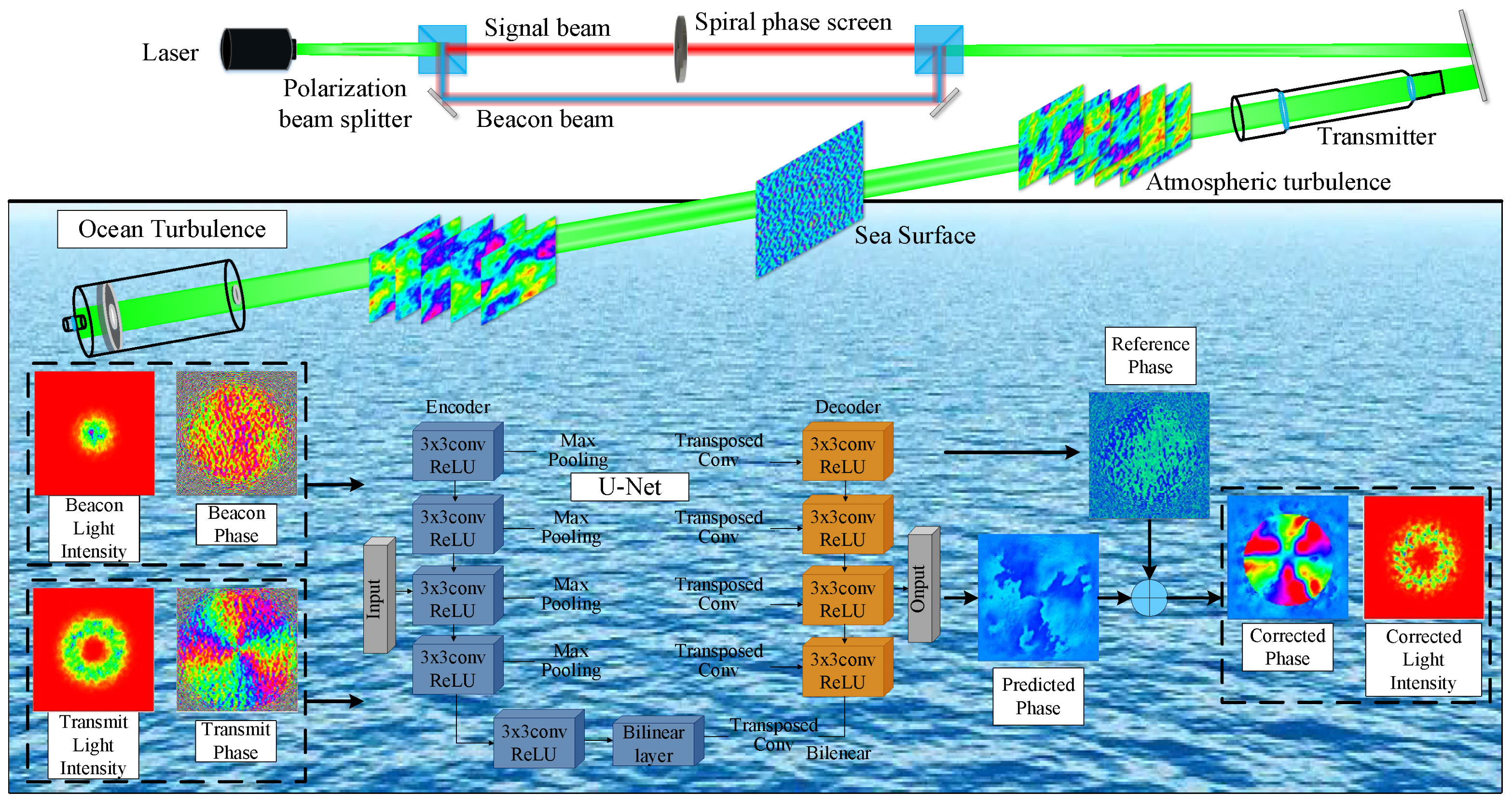
2.1. Modeling of Vortex Optical Transmedium Transport

The atmospheric turbulence model is constructed based on the modified Kolmogorov power spectral model, whose power spectral density function for refractive index undulation can be expressed as follows [26]:

$${\Phi }_n(\kappa )=0.033C_n^2{\kappa }^{-11/3}\left(1+2.35{(\kappa \eta )}^{2/3}\right)\exp \left(-{\kappa }^2/{\kappa }_l^2\right)$$

(1)

where κ is the spatial frequency, $C_n^2$ is the atmospheric refractive index structure constant, and for slant-range transmission, since the angle between the beam and the sea level is not zero, the atmospheric refractive index structure constant $C_n^2$ is a function of the distance h from the sea level height and is integrated and converted to an equivalent value along the slant-range direction [27]. η is the Kolmogorov internal scale, and κ_l = 3.3/η is the high-frequency cutoff wave number. The Fourier transform method is used to generate the high-frequency phase screen, and the complete phase screen is realized by multi-scale low-frequency compensation [28]:

$${\varphi }_{\mathrm{low}}(m,n)={\displaystyle \sum _{p=1}^{N_p}{\displaystyle \sum _{k,l=-3}^2{h}_{kl}^{(p)}}}\cdot 3^{-p}\cdot \exp \left[i2\pi \left({\displaystyle \frac{3^{-p}k\cdot m}{N_x}}+{\displaystyle \frac{3^{-p}l\cdot n}{N_y}}\right)\right]$$

(2)

where m, n are the discrete coordinates of the target phase screen, k, l are the subharmonic frequency indices, N_p = 3 is the number of compensation layers, N_x, N_yare the number of sampling points of the phase screen in the x and y directions, and $h_{kl}^{(p)}$ is the Hermitian symmetric complex Gaussian field, and the final total atmospheric phase screen is as follows:

$${\varphi }_{\mathrm{atm}}(x,y)\hspace{0.33em}=\hspace{0.33em}{\varphi }_{\mathrm{high}}(x,y)\hspace{0.33em}\oplus \hspace{0.33em}{\varphi }_{\mathrm{low}}(x,y)$$

(3)

where ‘⊕’ denotes element-wise (point-wise) addition in the phase domain. The modulation effect of dynamic sea surface waves is modeled using the JONSWAP spectrum with the directional spectrum expression [7]:

$$S(\omega ,\theta )=\alpha g^2{\omega }^{-5}\exp \left(-{\displaystyle \frac{5}{4}}{\left({\displaystyle \frac{{\omega }_p}{\omega }}\right)}^4\right){\gamma }^{\exp \left(-{\displaystyle \frac{{(\omega -{\omega }_p)}^2}{2{\sigma }^2{\omega }_p^2}}\right)}\cdot {\cos }^2\left(\theta -{\theta }_{\mathrm{mean}}\right)$$

(4)

where α = 0.0081, ω is the frequency, ω_p = g/U₁₀ is the peak frequency, σ is the JONSWAP spectral width, γ is the spectral sharpening parameter, θ is the azimuthal angle, and θ_mean is the main wind direction. The sea surface height field h(x,y) is generated by Fourier inversion and mapped to phase modulation [29]:

$${\varphi }_{\mathrm{sea}}\left(x,y\right)=\pi \cdot {\displaystyle \frac{h\left(x,y\right)}{\max \left(\left|h\right|\right)}}$$

(5)

where h(x, y) is the sea surface height field. The ocean turbulence phase screen is generated based on the Nikishov joint temperature-salinity perturbation spectrum with a power spectral density shown as follows [30]:

$${\Phi }_o(\kappa )=0.388\times {10}^{-8}{ϵ}^{-1/3}{\kappa }^{-11/3}{\displaystyle \frac{{\chi }_T}{{\omega }^2}}\left[{\omega }^2{e}^{-A_{t}s(\kappa )}+e^{-A_{s}s(\kappa )}-2\omega e^{-A_{ts}s(\kappa )}\right]$$

(6)

where s(κ) = 8.284(κη)^4/3 + 12.978(κη)², η is the Kolmogorov microscale, ϵ is the turbulence energy dissipation rate, and ϵ is considered as a function of the depth h and integrated in the direction of the slanting course to be the equivalent energy dissipation rate for the slanting course transport. χ_T is the temperature dissipation rate, and κ is the number of spatial waves. ω is the value that determines the contribution of the salinity and the temperature to turbulence, taking η = 1 × 10⁻³, A_T = 1.863 × 10⁻², A_S = 1.9 × 10⁻⁴, A_TS = 9.41 × 10⁻³, δ = 8.248(kη)^3/4 + 12.978(kη)².

According to the derivation of the sea-water refractive-index spectrum by Nikishov, the weighting parameters in Equation (6) are defined as follows [30]:

$$\eta ={\displaystyle \frac{C_n^2}{C_{n,\mathrm{atm}}^2}},\hspace{0.33em}\hspace{0.33em}\hspace{0.33em}{\Lambda }_T={\displaystyle \frac{{\omega }_T}{{\omega }_T+{\omega }_S}},\hspace{0.33em}\hspace{0.33em}\hspace{0.33em}{\Lambda }_S={\displaystyle \frac{{\omega }_S}{{\omega }_T+{\omega }_S}}.$$

(7)

The temperature and salinity contribution weights, ω_T and ω_S, are obtained from the turbulent-dissipation rates [30]:

$${\epsilon }_T=K_T{({\displaystyle \frac{\partial T}{\partial z}})}^2,\hspace{0.33em}\hspace{0.33em}\hspace{0.33em}{\epsilon }_S=K_S{({\displaystyle \frac{\partial S}{\partial z}})}^2,\hspace{0.33em}\hspace{0.33em}\hspace{0.33em}{\omega }_T={\displaystyle \frac{{\epsilon }_T}{{\epsilon }_T+{\epsilon }_S}},\hspace{0.33em}\hspace{0.33em}\hspace{0.33em}{\omega }_S={\displaystyle \frac{{\epsilon }_S}{{\epsilon }_T+{\epsilon }_S}}.$$

(8)

Assuming constant temperature gradient ΔT/H and salinity gradient ΔS/H within a layer of thickness H, these simplify to the following [30]:

$${\omega }_T={\displaystyle \frac{K_T{(\Delta T/H)}^2}{K_T{(\Delta T/H)}^2+K_S{(\Delta S/H)}^2}},\hspace{0.33em}\hspace{0.33em}\hspace{0.33em}{\omega }_S={\displaystyle \frac{K_S{(\Delta S/H)}^2}{K_T{(\Delta T/H)}^2+K_S{(\Delta S/H)}^2}}.$$

(9)

In our simulations, we adopt the following typical values from Nikishov, determined by experimental fitting: K_T = 1.4 × 10⁻⁷ m²/s, K_S = 7.0 × 10⁻¹⁰ m²/s, α = 2.6 × 10⁻⁴ K⁻¹, β = 1.75 × 10⁻⁴ psu⁻¹.

All of the ocean-turbulence parameters used in Equation (6)—including the temperature-dissipation coefficient K_T, the salinity-dissipation coefficient K_S, the refractive-index sensitivity coefficients α and β, and the spectrum shape parameters A_T and A_S—were adopted directly from Nikishov (2000) [30] without further calibration in this work (in their Equations (14)–(17)). No additional empirical fitting was performed in the present study.

The phase screen generation process also uses power spectrum inversion with multiscale layered low-frequency compensation, and the final superposition is as follows:

$${\varphi }_{\mathrm{ocean}}(x,y)\hspace{0.33em}=\hspace{0.33em}{\varphi }_{\mathrm{high}\_\mathrm{ocean}}(x,y)\hspace{0.33em}\oplus \hspace{0.33em}{\varphi }_{\mathrm{low}\_\mathrm{ocean}}(x,y)$$

(10)

The optical field transmission is realized by segmentation of the angular spectral method, and the transmission function corresponding to the propagation distance Δz for each segment is as follows [31]:

$$H(f_x,f_y)=\exp \left(-i\pi \lambda \Delta z\left(f_x^2+f_y^2\right)\right)$$

(11)

where f_x, f_y are the transverse spatial frequency components, λ is the wavelength, and Δz is the propagation distance between two neighboring phase screens. The transmission process iteratively updates the light field by applying the cumulative phase perturbation:

$${\varphi }_{\mathrm{total}}={\varphi }_{\mathrm{atm}}(x,y)\hspace{0.33em}\oplus \hspace{0.33em}{\varphi }_{\mathrm{sea}}(x,y)\hspace{0.33em}\oplus \hspace{0.33em}{\varphi }_{\mathrm{ocean}}(x,y)$$

(12)

(notation only; applied sequentially) In practice, the field is first multiplied by exp[iϕ_atm(x,y)] and propagated over Δz via the atmospheric angular spectral transfer function H_atm, then the resulting field is modulated by exp[iϕ_sea(x,y)] at the sea-surface interface (no angular spectral propagation applied here), and finally multiplied by exp[iϕ_ocean(x,y)] and propagated over Δz via H_ocean to reach the next phase-screen position [32]:

$$u(x,y,z+\Delta z)={\mathcal{F}}^{-1}\left[\mathcal{F}\left(u\cdot e^{i{\varphi }_{\mathrm{s}}}\right)\cdot H\right],\mathrm{s}=\mathrm{a}\mathrm{t}\mathrm{m} \mathrm{o}\mathrm{r} \mathrm{o}\mathrm{c}\mathrm{e}\mathrm{a}\mathrm{n}$$

(13)

where u(x,y,z) is the distribution of the complex amplitude light field at the longitudinal coordinate z, $\mathcal{F}$ and ${\mathcal{F}}^{-1}$ is the Fourier transform and inverse Fourier transform. The parameters of the proposed transmedia transport model are set as follows: wavelength λ = 530 nm, grid resolution N = 128, spatial window L = 0.4 m, an atmospheric transmission distance of 1000 m, an oceanic transmission distance of 10 m, number of atmospheric segments = 100, number of oceanic segments = 5. The framework realizes the high-precision simulation of the atmospheric–oceanic transmedia perturbation through the combination of physical constraints and numerical optimization.

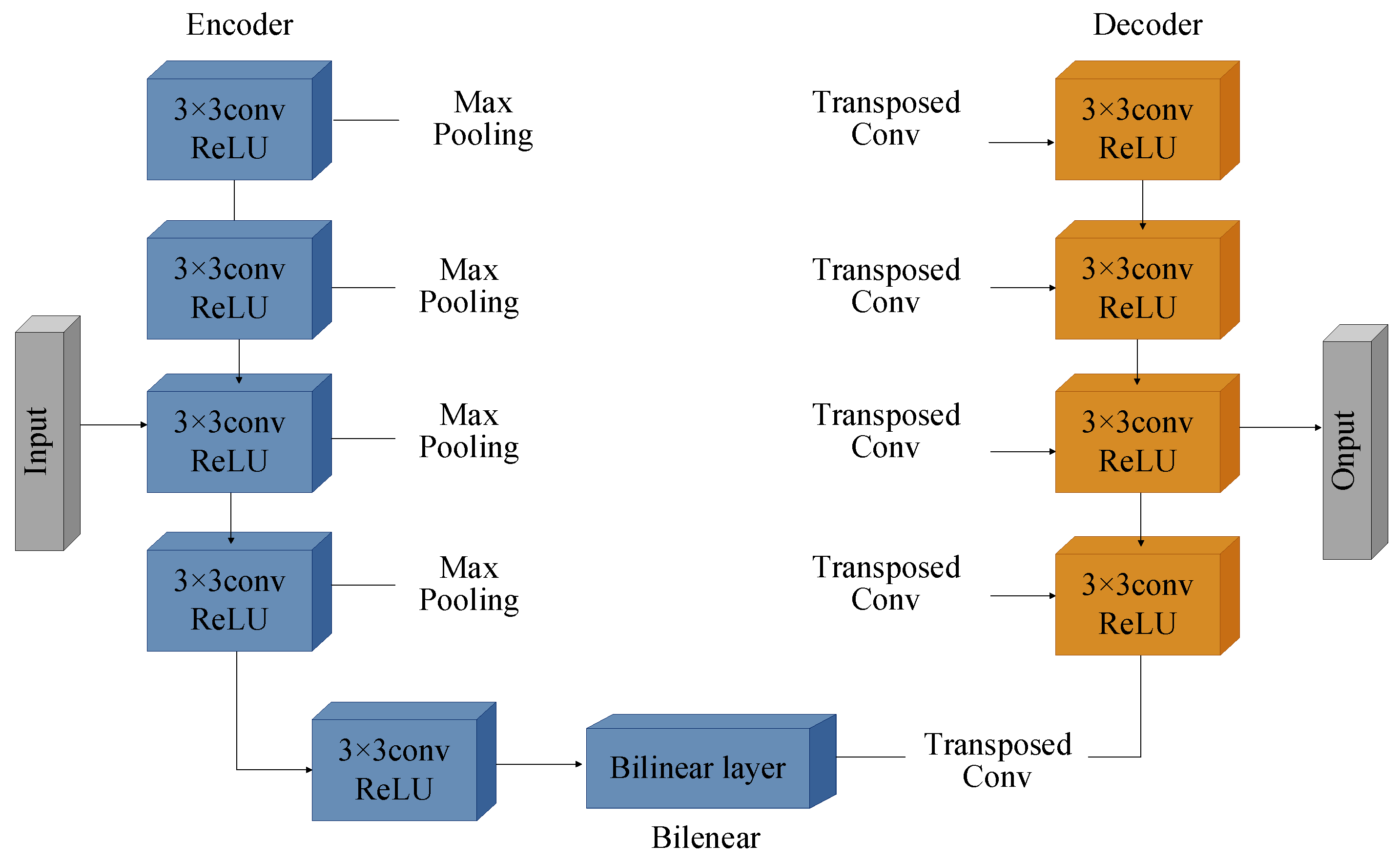
2.2. Phase Prediction Method Based on Improved U-Net

We leverage an enhanced U-Net with multi-channel feature fusion to directly recover vortex-beam wavefront phases from intensity images distorted by cross-media turbulence. By integrating physics-guided feature engineering into a lightweight network design, our model delivers robust phase estimation even under severe turbulent conditions.

The dataset is generated using a hybrid parameterization approach covering different atmospheric turbulence intensities ($C_n^2$ ∈ [10⁻²⁰, 10⁻¹⁵] m^−2/3), ocean turbulence dissipation rates (ϵ ∈ [10⁻¹⁷, 10⁻¹⁵] m^−2/3) and sea surface wind speeds (U₁₀ ∈ [0.1, 0.7] m/s) to ensure that the model is sensitive to the dynamic complexity of the environment. Before training, the input light intensity images and phase labels are uniformly normalized: the light intensity part is normalized by Z-score, and the phase values are linearly mapped from the initial [−π, π] to the [0, 1] interval to stabilize the gradient and accelerate the network convergence. A multi-channel feature-extraction strategy is proposed, in which the input tensor is enriched with physically informed channels spatial intensity gradients, Fourier-domain spectral descriptors and multi-scale filter responses to enable adaptive capture of implicit higher-order OAM mode characteristics and high-frequency phase perturbations induced by atmospheric and oceanic turbulence, thereby substantially enhancing model robustness and phase-recovery accuracy under complex distortion conditions. First, the raw light intensity images are log-transformed to compress the dynamic range, and the luminance differences are eliminated by global normalization [33]:

$$I_{\log }(x,y)={\displaystyle \frac{{\log }_{10}\left(I\left(x,y\right)+\zeta \right)-{\mu }_{\log }}{{\sigma }_{\log }}}$$

(14)

where I(x,y) is the gray value of the original light intensity image at pixel(x,y), ζ = 10⁻⁸ is a small dimensionless constant added to avoid log₁₀(0) singularities, and μ_log and σ_log are the mean and standard deviation of the log-transformed intensities over the training set. Next, the gradient magnitude of the log light intensity is computed to capture the edge information of the phase mutation region [33]:

$$G(x,y)=\sqrt{{\left({\displaystyle \frac{\partial I_{\log }}{\partial x}}\right)}^2+{\left({\displaystyle \frac{\partial I_{\log }}{\partial y}}\right)}^2}$$

(15)

The frequency domain features are further extracted by fast Fourier transform, and the amplitude is log-normalized as follows [34]:

$$F_{\mathrm{norm}}(x,y)={\displaystyle \frac{\log \left(1+|\mathcal{F}(I_{\log })|\right)-{\mu }_F}{{\sigma }_F}}$$

(16)

where μ_F, σ_F are the mean and standard deviation of the log amplitude of the training set spectrum. Finally, I_log is filtered using a multi-scale Gaussian kernel (σ∈ {1, 2, 4, 8}) to extract the turbulence structure at different spatial frequencies:

$$M_{\sigma }\left(x,y\right)=I_{\log }\ast G_{\sigma }$$

(17)

$$G_{\sigma }\left(x,y\right)={\displaystyle \frac{1}{2\pi {\sigma }^2}}\exp \left(-{\displaystyle \frac{x^2+y^2}{2{\sigma }^2}}\right)$$

(18)

where σ is the Gaussian kernel standard deviation and * is the convolution symbol. The four types of features mentioned above are spliced along the channel dimensions to form the input tensor X∈R^H×W×7, where H = 128 and W = 128 are the image dimensions. Figure 2 shows the complete processing flow from input light intensity to multi-channel features.

Our modified U-Net employs a five-level encoder–decoder architecture (Figure 3). In each encoding stage, two consecutive 3 × 3 convolutions with “same” zero padding and ReLU activations are applied, followed by 2 × 2 max-pooling for spatial down-sampling and multiscale feature extraction. At the network bottleneck, depthwise-separable convolutions reduce parameter count without sacrificing representational capacity. In the decoding path, feature maps are up-sampled via 2 × 2 transposed convolutions and concatenated with their corresponding encoder features through skip connections; two additional 3 × 3 convolutions with ReLU activations then progressively restore high-resolution phase information. A final 1 × 1 convolution projects the feature maps to phase estimates ϕ∈[−π, π], which are optimized directly using a regression loss. Training is performed with the Adam optimizer (initial learning rate = 1 × 10⁻⁴, batch size = 32) for up to 500 epochs. The dataset used for phase-prediction was partitioned into 70% training, 15% validation, and 15% test subsets.

To simultaneously optimize the phase global distribution with local details, the loss function L_total is combined with the mean-square error L_MSE and the gradient difference loss L_grad [35]:

$$L_{\mathrm{MSE}}={\displaystyle \frac{1}{N}}{\displaystyle \sum _{i=1}^N\Vert {\varphi }_i-{\widehat{\varphi }}_i{\Vert }_2^2}$$

(19)

$$L_{\mathrm{grad}}={\displaystyle \frac{1}{N}}{\displaystyle \sum _{i=1}^N\Vert \nabla {\varphi }_i-\nabla {\widehat{\varphi }}_i{\Vert }_1}$$

(20)

where N is the number of small batch samples, ϕ_i is the column vector of all pixels in the ith true phase map, ${\widehat{\varphi }}_i$ denotes the column vector of the ith network predicted phase map, and ∇ϕ denotes the phase gradient. The total loss function is the weighted sum of the two [35]:

$$L_{\mathrm{total}}={\lambda }_1{L}_{\mathrm{MSE}}+{\lambda }_2{L}_{\mathrm{grad}}$$

(21)

The loss weights λ₁ = 1.0 and λ₂ = 0.5 were selected via grid search. As shown in Figure 4, the training loss curve exhibits three characteristic phases. During the initial epochs, the total loss decreases by approximately two orders of magnitude, reflecting rapid capture of low-frequency dominant phase perturbations through the multi-scale feature fusion. Between epochs 50 and 300, the loss plateaus around 8.5 ± 2.3 with periodic oscillations, indicating near-convergence on mid-frequency components and continued exploration of local minima. Beyond epoch 300, the loss resumes an exponential decay, ultimately reaching its global minimum by epoch 500.

3. Results and Discussion

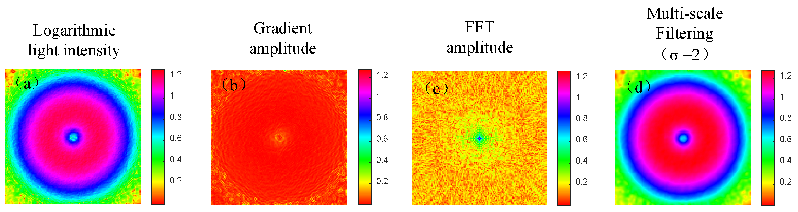
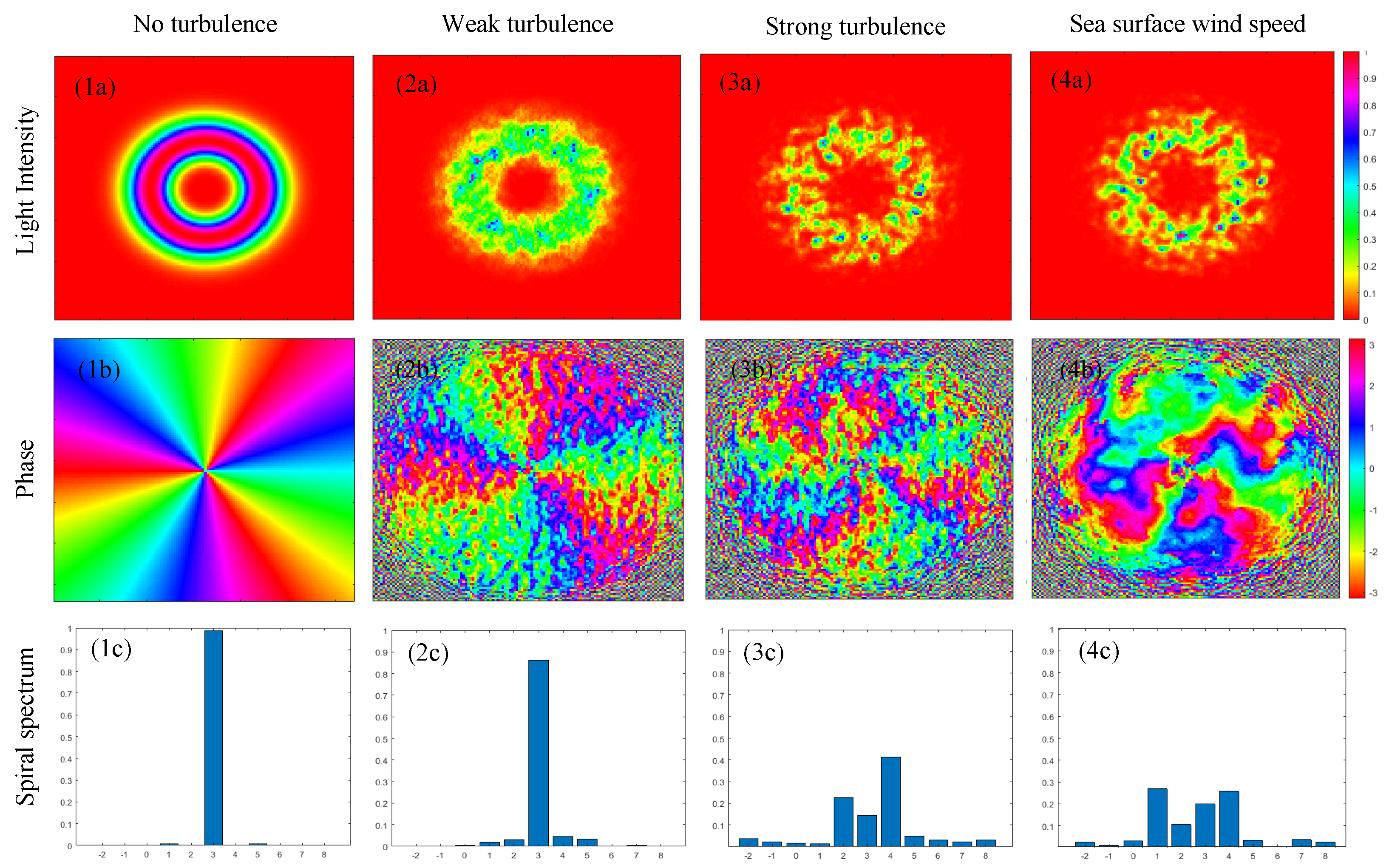
3.1. Transmission Characterization

Figure 5 presents, for an l = 3 vortex beam, the spatial intensity profiles, phase maps, and helical-mode spectra in the unperturbed state and after propagation through various hybrid atmospheric–oceanic channels, as simulated by our hierarchical phase-screen and dynamic sea-surface modulation models.

For a vortex beam of wavelength λ = 530 nm propagating without turbulence, the intensity exhibits a clean annular profile with normalized peak = 1 and the phase map shows the characteristic helical gradient (−π to π). The OAM spectrum concentrates 98.5% of the power in the target mode (l = 3), with the remaining 1.5% leakage attributable to spectral truncation (l = −3 to 9). Under weak turbulence ($C_n^2$ = 1 × 10⁻¹⁶ m^−2/3, ϵ = 1 × 10⁻¹⁶ m²/s³, U₁₀ = 0.2 m/s), the ring structure persists with slight edge scattering; localized phase–gradient breaks arise from low-frequency atmospheric perturbations; and the l = 3 power share drops to 86.1%, while l = 2 and l = 4 components increase to 3.1% and 4.4%, respectively. Under strong turbulence ($C_n^2$ = 1 × 10⁻¹⁵ m^−2/3, ϵ = 1 × 10⁻¹⁵ m²/s³, U₁₀ = 0.2 m/s), the intensity becomes fully decoherent and randomly scattered, and the phase is severely disrupted by combined high-frequency atmospheric and anisotropic oceanic aberrations; the l = 3 share falls to 41.2%, with side-mode contributions of l = 2 (22.4%), l = 4 (14.5%) and l = 5 (4.7%). Further increasing the sea-surface wind speed to U₁₀ = 0.7 m/s under strong turbulence exacerbates high-frequency phase noise, asymmetrically spreads the intensity distribution, reduces l = 3 power to 19.8%, and elevates sidelobe modes to l = 1 (26.9%), l = 2 (10.6%) and l = 4 (25.7%).

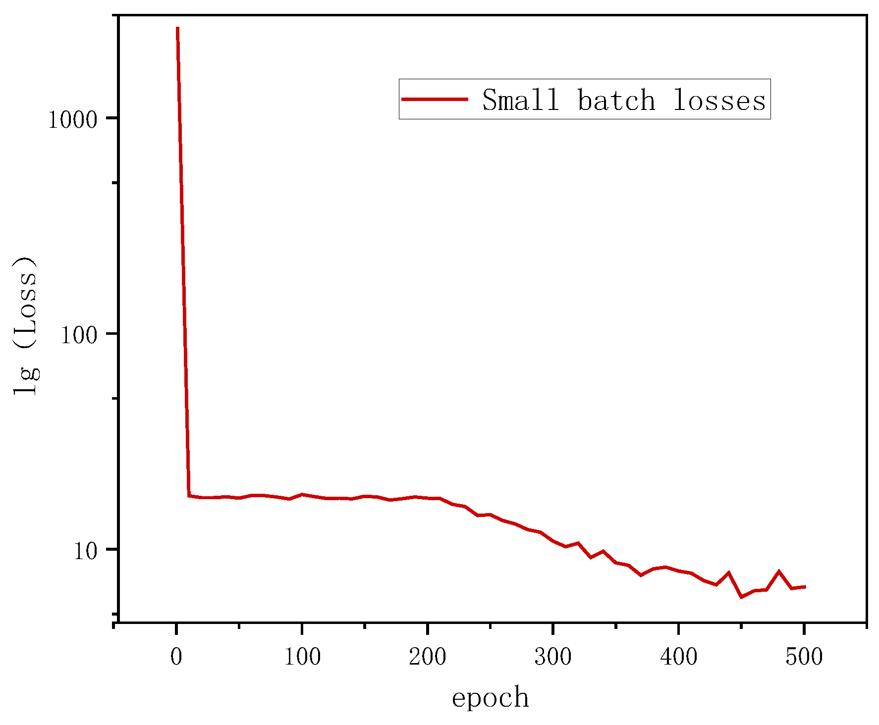
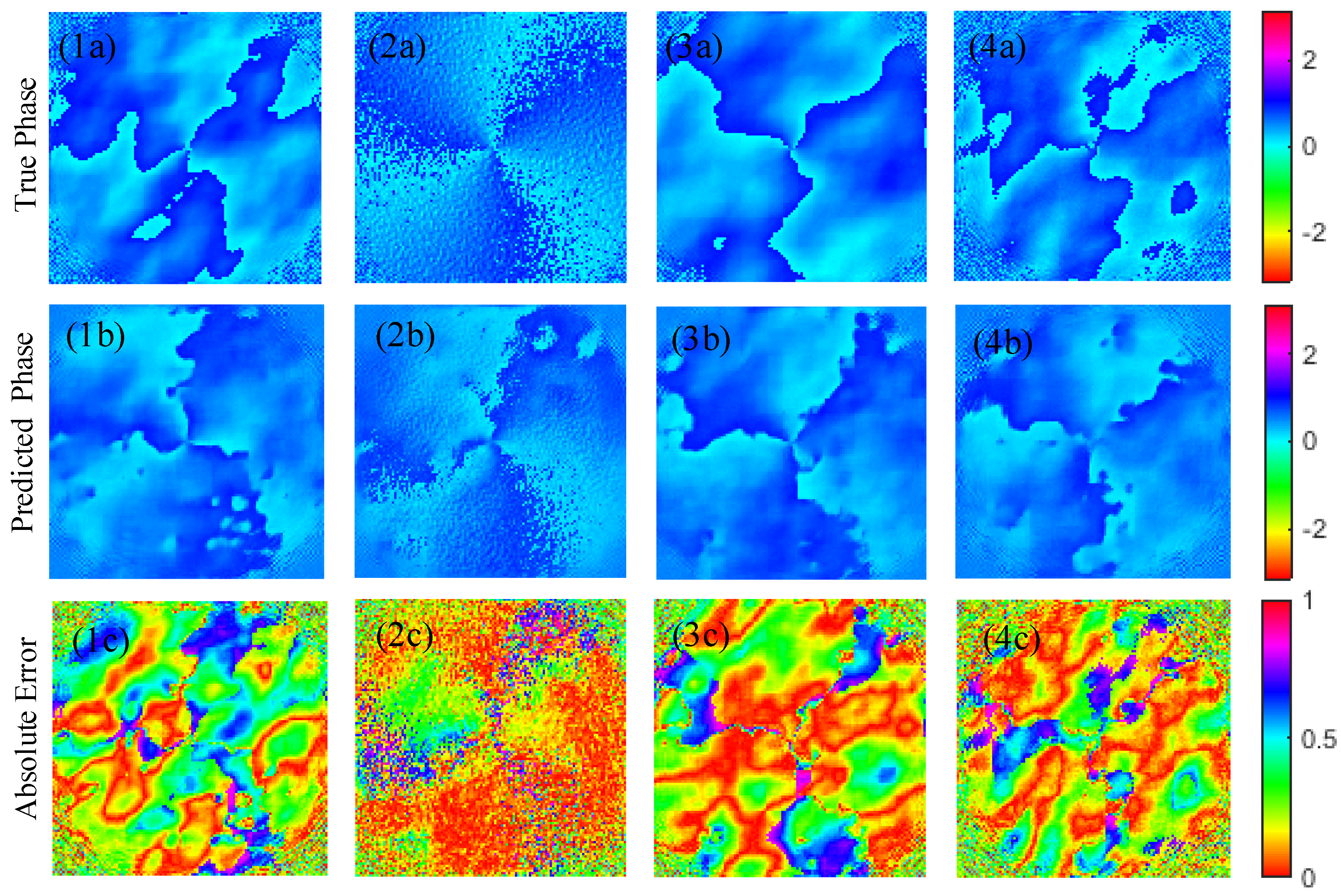
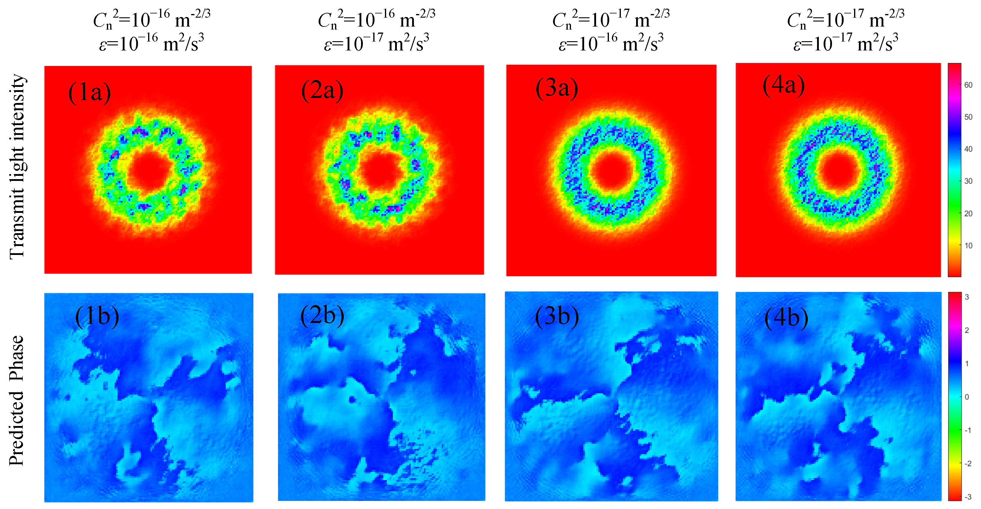
3.2. U-Net Phase Prediction Model

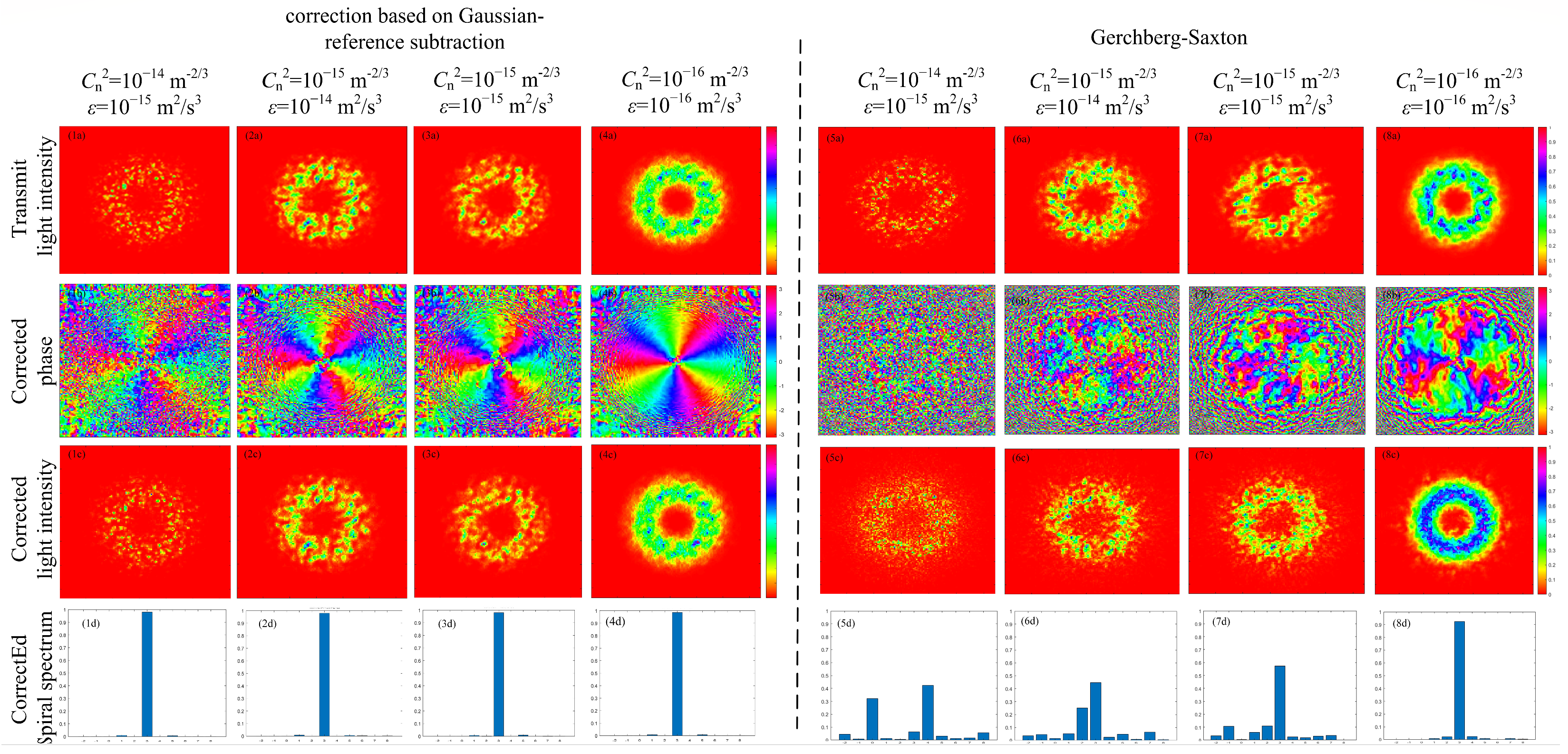
A hybrid parameterization method as in Section 2.2 is used to divide the training set and validation set in a ratio of 4:1. The input light intensity is preprocessed using the image processing method described in Section 2.2, and the final seven-channel input tensor is constructed.

In the performance validation process, the performance of the prediction model is quantified using pixel-level root-mean-square error (RMSE) on the training and validation sets, which is defined as follows:

$$\mathrm{RMSE}=\sqrt{{\displaystyle \frac{1}{N\cdot H\cdot W}}{\displaystyle \sum _{i=1}^N{\displaystyle \sum _{x=1}^H{\displaystyle \sum _{y=1}^W{\left[{\varphi }_{\mathrm{true},i}\left(x,y\right)-{\varphi }_{\mathrm{pred},\mathrm{i}}\left(x,y\right)\right]}^2}}}}$$

(22)

where N is the number of images in the validation set (or training set), ϕ_true is the true phase, and ϕ_pred is the predicted phase. The root-mean-square error (RMSE) decreased from 72.07 and 69.43 rad in the untrained state to 4.03 and 7.16 rad after training, respectively. Randomly selected validation examples further demonstrate the model’s strong generalization performance. Figure 6 presents the ground-truth and predicted phase maps alongside their absolute-error distributions. The error maps show that the network accurately reconstructs the vortex wavefront structure over most regions, with residual aberrations confined to localized zones under strong turbulence. These results confirm the framework’s robust recovery capability in complex perturbation conditions, while also highlighting the need for improved reconstruction of fine-scale phase details.

Figure 7 compares the distorted intensity profiles and U-Net–predicted phase maps for l = 3 vortex beams under four turbulence conditions. In panel (a), as $C_n^2$ and ϵ increase, the characteristic annular intensity becomes progressively blurred. In panel (b), the U-Net successfully reconstructs the primary helical phase structure; however, local aberrations—especially near the ring edges and singularity core—persist. With stronger turbulence, the continuity of the spiral fringe degrades, and absolute phase errors amplify in these regions. These results demonstrate the model’s ability to recover bulk wavefront features in complex perturbations while indicating that finer-scale phase reconstruction remains an avenue for further improvement.

In order to place the performance of our U-Net phase-prediction model in a broader context, we additionally evaluated a lightweight LSTM-based network under the same training and validation conditions. The LSTM architecture—while conceptually capable of capturing spatial dependencies via its recurrent units—achieved a validation RMSE of 7.10 rad, which is effectively on par with the U-Net’s 7.16 rad, yet demanded roughly five times the number of parameters and exhibited an inference latency of approximately 50 ms per frame compared to the U-Net’s 10 ms. This substantial increase in computational complexity, without any meaningful accuracy gain, indicates that the LSTM approach does not offer a practical advantage for real-time cross-media phase recovery.

Moreover, to isolate the impact of our physics-informed preprocessing pipeline, we conducted a controlled ablation in which we removed all multi-channel feature extraction and fed only the raw intensity image into the U-Net, keeping the network architecture and training hyperparameters unchanged. Under these conditions, the validation RMSE rose to 8.94 rad—an approximate 25% degradation in performance. This result highlights the critical importance of our carefully designed preprocessing steps in enabling robust, high-fidelity phase reconstruction in complex turbulent channels.

3.3. Closed-Loop

A feed-forward correction based on Gaussian-reference subtraction is used and analyzed in comparison with the classical Gerchberg–Saxton phase recovery algorithm [13]. Under turbulent disturbance conditions, the feed-forward correction based on Gaussian-reference subtraction method can effectively reduce the prediction error and gradually restore the target phase structure.

In the corrected spiral spectrum, the power share of the target mode (l = 3) is increased from 38.4% to 98.1%, and the power of the side-phase mode l = 1 is reduced to 0.6%. This result shows that the feed-forward correction based on Gaussian-reference subtraction method not only improves the energy concentration of the target mode by optimizing the phase recovery process, but also effectively reduces the crosstalk between modes and enhances the transmission quality of the vortex beam. Under weak turbulence conditions, the spiral spectrum target power of the aberrated optical field is 92.4%, which is improved to 98.7% after correction, and the parabolic mode l = 1 power is reduced from 18.3% to 0.8%. Under strong turbulence conditions, the power share of the target mode (l = 3) is enhanced from 3.2% to 97.3%, as shown in Figure 8(a1–d4). To demonstrate the robustness and reproducibility of this approach, we conducted 1000 independent simulations under identical strong-turbulence conditions, each driven by a distinct random phase screen. Across all trials, the uncorrected target-mode (l = 3) power share averaged 38.4% with a standard deviation of 3.1%, whereas after reference-subtraction correction it rose to 98.1% with a standard deviation of 1.2%. The results confirmed that the observed gain is neither anecdotal nor confined to a particular realization, but is instead a consistent, statistically significant effect of our correction framework. These results underscore that the proposed one-step Gaussian-reference subtraction not only simplifies the correction process by eliminating iterative loops and prior mode knowledge, but also delivers reliable and repeatable enhancement of the vortex mode’s energy concentration under severe cross-media turbulence.

The Gerchberg–Saxton algorithm employs an alternating-projection approach for phase retrieval, with correction performance hinging on the initial phase estimate. Over 500 iterations, it elevates the target-mode power from 49.4% to 57.3% while reducing the l = 4 sidelobe from 7.3% to 2.4%. Under weak turbulence, the algorithm boosts l = 3 power from 92.3% to 94.6%, maintaining all sidelobe contributions below 1%. However, in strong-turbulence conditions, it achieves only a modest increase in target power—from 1% to 6.4%—as shown in Figure 8(a5–d8).

Under weak turbulence, both Gerchberg–Saxton and our feed-forward correction based on Gaussian-reference subtraction method effectively concentrate energy in the target OAM mode and suppress sidelobes, yielding comparable accuracy. In contrast, under severe turbulence with pronounced sea-surface dynamics, Gerchberg–Saxton’s reliance on its initial guess often leads to entrapment in local optima and limited mode recovery. By leveraging the U-Net’s initial phase prediction and incorporating an error-feedback loop, the feed-forward correction based on Gaussian-reference subtraction scheme iteratively refines the phase estimate, enhancing target-mode power even in extreme conditions. These findings demonstrate that feed-forward correction based on the Gaussian-reference subtraction method, grounded in deep-network priors and closed-loop optimization, offers superior adaptability and robustness across diverse cross-media perturbation environments, underscoring its practical value for real-time optical communication systems.

From a computational-complexity standpoint, the Gerchberg–Saxton algorithm incurs O(N·logN) operations per iteration—where N = 128 × 128 = 16,384 pixels, and the number of iteration rounds is usually as high as a few hundred, for a total workload of roughly 1.15 × 10⁸ operations. In contrast, our Gaussian-reference subtraction scheme consists of a single U-Net forward pass of complexity O(D·N) (D = 40 effective layers), followed by one element-wise subtraction of two N-pixel phase maps—an additional O(N) cost. The total cost thus remains on the order of O(D·N), amounting to approximately 1.47 × 10⁶ operations. Consequently, Gaussian-reference subtraction achieves markedly higher computational efficiency and parallelism, making it far better suited to real-time cross-media optical communication scenarios while retaining comparable correction accuracy.

4. Conclusions and Outlook

In this work, we address phase aberrations of vortex beams in hybrid atmospheric–oceanic channels by introducing a hybrid correction framework that synergizes hierarchical phase-screen modeling, a lightweight U-Net with multi-channel feature fusion, and a feed-forward correction based on Gaussian-reference subtraction. Our results demonstrate a substantial improvement in wavefront recovery accuracy under complex perturbation conditions. Future studies will adapt and extend this framework to compiled-code optical communication systems, with vortex beam modulation as the principal application focus. Although our current implementation focuses on high-fidelity simulation, future work will address the practical realization of this pipeline on hardware. We aim to demonstrate real-time phase recovery through live optical measurements and closed-loop correction in a laboratory setting.

References

1. Allen, L.; Beijersbergen, M.W.; Spreeuw, R.J.C.; Woerdman, J.P. Orbital angular momentum of light and the transformation of Laguerre-Gaussian laser modes. Phys. Rev. A 1992, 45, 8185. [Google Scholar] [CrossRef]
2. Cheng, M.; Jiang, W.; Guo, L.; Li, J.; Forbes, A. Metrology with a twist: Probing and sensing with vortex light. Light Sci. Appl. 2025, 14, 4. [Google Scholar] [CrossRef]
3. Li, S.; Chen, S.; Gao, C.; Willner, A.E.; Wang, J. Atmospheric turbulence compensation in orbital angular momentum communications: Advances and perspectives. Opt. Commun. 2018, 408, 68–81. [Google Scholar] [CrossRef]
4. Hasselmann, D.E.; Dunckel, M.; Ewing, J.A. Directional wave spectra observed during JONSWAP 1973. J. Phys. Oceanogr. 1980, 10, 1264–1280. [Google Scholar] [CrossRef]
5. Wang, X.; Ma, Y.; Yuan, Q.; Chen, W.; Wang, L.; Zhao, S. Properties of focused Laguerre-Gaussian beam propagating in anisotropic ocean turbulence. Chin. Phys. B 2024, 33, 024208. [Google Scholar] [CrossRef]
6. Zhan, H.; Wang, L.; Peng, Q.; Wang, W.; Zhao, S. Progress in adaptive optics wavefront correction technology of vortex beam (Invited). Infrared Laser Eng. 2021, 50, 20210428. [Google Scholar]
7. Brüning, C.; Alpers, W.; Hasselmann, K. Monte-Carlo simulation studies of the nonlinear imaging of a two dimensional surface wave field by a synthetic aperture radar. Int. J. Remote. Sens. 1990, 11, 1695–1727. [Google Scholar] [CrossRef]
8. Xu, Y.; Shi, H.; Zhang, Y. Effects of anisotropic oceanic turbulence on the power of the bandwidth-limited OAM mode of partially coherent modified Bessel correlated vortex beams. J. Opt. Soc. Am. A 2018, 35, 1839–1845. [Google Scholar] [CrossRef]
9. Aghajani, A.; Kashani, F.D.; Yousefi, M. Laboratory study of aberration calculation in underwater turbulence using Shack-Hartmann wavefront sensor and Zernike polynomials. Opt. Express 2024, 32, 15978–15992. [Google Scholar] [CrossRef]
10. Yang, H.; Zang, X.; Zhang, Z.; Liu, J. Wavefront correction system based on RUN optimization algorithm. Acta Photon. Sin. 2023, 52, 1111004. [Google Scholar]
11. Zhao, S.M.; Leach, J.; Gong, L.Y.; Ding, J.; Zheng, B.Y. Aberration corrections for free-space optical communications in atmosphere turbulence using orbital angular momentum states. Opt. Express 2011, 20, 452–461. [Google Scholar] [CrossRef] [PubMed]
12. Yang, H.; Su, H.; Zhang, Z. Wavefront correction based on KL modes by SPGD control algorithm. Chin. J. Lasers 2023, 50, 1405001. [Google Scholar]
13. Basu, D.; Chejarla, S.; Maji, S.; Bhattacharya, S.; Srinivasan, B. An adaptive optical technique for structured beam generation based on phase retrieval using modified Gerchberg–Saxton algorithm. Opt. Laser Technol. 2024, 170, 110244. [Google Scholar] [CrossRef]
14. Nishizaki, Y.; Valdivia, M.; Horisaki, R.; Kitaguchi, K.; Saito, M.; Tanida, J.; Vera, E. Deep learning wavefront sensing. Opt. Express 2019, 27, 240–251. [Google Scholar] [CrossRef]
15. Lu, C.; Tian, Q.; Zhu, L.; Gao, R.; Yao, H.; Tian, F.; Zhang, Q.; Xin, X. Mitigating the ambiguity problem in the CNN-based wavefront correction. Opt. Lett. 2022, 47, 3251–3254. [Google Scholar] [CrossRef]
16. Wu, Y.; Guo, Y.; Bao, H.; Rao, C. Sub-Millisecond Phase Retrieval for Phase-Diversity Wavefront Sensor. Sensors 2020, 20, 4877. [Google Scholar] [CrossRef]
17. Liu, W.; Luo, J.; Yang, Y.; Wang, W.; Deng, J.; Yu, L. Automatic lung segmentation in chest X-ray images using improved U-Net. Sci. Rep. 2022, 12, 8649. [Google Scholar] [CrossRef]
18. Fan, C.; Chen, Z.; Lin, H.; Wang, X. TCGFusion: A network for PET-MRI fusion based on GAN and transformer. Multimed. Tools Appl. 2024, 83, 37505–37522. [Google Scholar] [CrossRef]
19. Zhao, Z.Q.; Zheng, P.; Xu, S.; Wu, X. Object detection with deep learning: A review. IEEE Trans. Neural Netw. Learn. Syst. 2019, 30, 3212–3232. [Google Scholar] [CrossRef]
20. Guo, H.; Tang, W.; Wang, Z.; Yuan, L.; Li, Y.; He, D.; Wang, Q.; Huang, Y. Liquid crystal wavefront correction based on improved machine learning for free-space optical communication. Appl. Opt. 2023, 62, 9470–9475. [Google Scholar] [CrossRef]
21. Tian, Q.; Lu, C.; Liu, B.; Zhu, L.; Pan, X.; Zhang, Q.; Yang, L.; Tian, F.; Xin, X. DNN-based aberration correction in a wavefront sensorless adaptive optics system. Opt. Express 2019, 27, 10765–10776. [Google Scholar] [CrossRef]
22. Ma, H.; Liu, H.; Qiao, Y.; Li, X.; Zhang, W. Numerical study of adaptive optics compensation based on Convolutional Neural Networks. Opt. Commun. 2019, 433, 283–289. [Google Scholar] [CrossRef]
23. Fan, W.-Q.; Gao, F.-L.; Xue, F.-C.; Guo, J.-J.; Xiao, Y.; Gu, Y.-J. Experimental recognition of vortex beams in oceanic turbulence combining the Gerchberg–Saxton algorithm and convolutional neural network. Appl. Opt. 2024, 63, 982–989. [Google Scholar] [CrossRef] [PubMed]
24. Zhan, H.; Wang, L.; Wang, W. Generative adversarial network based adaptive optics scheme for vortex beam in oceanic turbulence. J. Light. Technol. 2022, 40, 4129–4135. [Google Scholar] [CrossRef]
25. Liu, J.; Du, Q.; Liu, F.; Wang, K.; Yu, J.; Wei, D. Vortex beam phase correction based on deep phase estimation network. Acta Opt. Sin. 2023, 43, 0601013. [Google Scholar]
26. Andrews, L.C.; Phillips, R.L. Laser Beam Propagation Through Random Media; SPIE Press: Bellingham, WA, USA, 2003. [Google Scholar]
27. Yang, S.; Li, M.; Ke, C.; Ding, D.; Ke, X. Coherent demultiplexing of vortex beam multiplexing transmission. Acta Opt. Sin. 2023, 43, 2006003. [Google Scholar]
28. Liu, T.; Zhu, C.; Sun, C.; Zhang, J.; Lei, Y.; Zhang, R. Improved subharmonic method for simulation of atmospheric turbulence phase screen. Acta Photon. Sin. 2019, 48, 0201002. [Google Scholar]
29. Su, D.; Wu, S.; Liu, L.; Liu, L. Ocean wave spectrum modeling-based sea surface polarization simulation. Laser Optoelectron. Prog. 2021, 58, 1411001. [Google Scholar]
30. Nikishov, V.I. Spectrum of turbulent fluctuations of the sea-water refraction index. Int. J. Fluid Mech. Res. 2000, 27, 82–98. [Google Scholar] [CrossRef]
31. Yin, K.; Huang, Z.; Lin, W.; Xing, T. Digital simulation of diffraction optical elements based on diffraction angular spectrum theory. Opto-Electron. Eng. 2012, 39, 125–128. [Google Scholar]
32. Fan, Z.; Song, Q.; Li, J.; Tankam, P. The study of color digital holography free from the zero-order diffraction interruption. Acta Phys. Sin. 2011, 60, 034204. [Google Scholar] [CrossRef]
33. Fan, R.; Hao, J.; Chen, R.; Wang, J.; Lin, Y.; Jin, J.; Yang, R.; Zheng, X.; Wang, K.; Lin, D.; et al. Phase retrieval based on deep learning with bandpass filtering in holographic data storage. Opt. Express 2024, 32, 4498–4510. [Google Scholar] [CrossRef]
34. Li, R.; Pedrini, G.; Huang, Z.; Reichelt, S.; Cao, L. Physics-enhanced neural network for phase retrieval from two diffraction patterns. Opt. Express 2022, 30, 32680–32692. [Google Scholar] [CrossRef]
35. Cao, Y.; Zhang, Z.; Peng, X. Wavefront distortion restoration method based on residual attention network. Acta Photon. Sin. 2022, 51, 1206002. [Google Scholar]
Figure 1. Overall system structure.
Photonics 12 00780 g001
Figure 2. Multi-channel feature processing. (a) Log light intensity. (b) Gradient magnitude. (c) FFT magnitude. (d) Multi-scale filtering.
Photonics 12 00780 g002
Figure 3. U-Net network structure.
Photonics 12 00780 g003
Figure 4. Training loss curve.
Photonics 12 00780 g004
Figure 5. Variation in light field after turbulent transport: (1a4a) light intensity; (1b4b) phase; (1c4c) spiral spectrum.
Photonics 12 00780 g005
Figure 6. Verification set test: (1a4a) true phase;. (1b4b) predicted phase; (1c4c) absolute error.
Photonics 12 00780 g006
Figure 7. U-Net network predicted phase. (1a4a) Light intensity after transmission. (1b4b) Predicted phase.
Photonics 12 00780 g007
Figure 8. Comparison of calibration methods: (1a8a) transmitted light intensity; (1b8b) calibrated phase; (1c8c) calibrated light intensity; (1d8d) calibrated spiral spectrum.
Photonics 12 00780 g008
Disclaimer/Publisher’s Note: The statements, opinions and data contained in all publications are solely those of the individual author(s) and contributor(s) and not of MDPI and/or the editor(s). MDPI and/or the editor(s) disclaim responsibility for any injury to people or property resulting from any ideas, methods, instructions or products referred to in the content.