Abstract
Optical solitons have emerged as a highly active research domain in nonlinear fiber optics, driving significant advancements and enabling a wide range of practical applications. This study investigates the dynamics of dark solitons in systems governed by the resonant nonlinear Schrödinger equation (RNLSE). For the RNLSE with third-order (3OD) and fourth-order (4OD) dispersions, the dark soliton solution of the equation in the (1+1)-dimensional case is derived using the F-expansion method, and the analytical study is extended to the (2+1)-dimensional case via the self-similar method. Subsequently, the nonlinear equation incorporating perturbation terms is further studied, with particular attention given to the dark soliton solutions in both one and two dimensions. The soliton dynamics are illustrated through graphical representations to elucidate their propagation characteristics. Finally, modulation instability analysis is conducted to evaluate the stability of the nonlinear system. These theoretical findings provide a solid foundation for experimental investigations of dark solitons within the systems governed by the RNLSE model.
1. Introduction
As an important class of nonlinear physical phenomena, solitons exhibit unique mathematical properties and physical behaviors. Solitons have been discovered and studied in many branches of physics, including optics [1]. Solitons have found widespread applications across various domains, including plasma physics [2], nonlinear optics [3], fluid dynamics [4], and fiber laser technologies [5]. In 1973, the use of solitons in optical fibers for optical communications was proposed by Hasegawa [6]. Their stable propagation characteristics make them well-suited for long-distance and high-capacity data transmission [7]. In particular, dark solitons, as an important type of soliton, have advanced properties that have made them increasingly prominent in the field of optical communication [8]. Additionally, soliton dynamics are increasingly being explored in emerging areas such as optical computing, quantum communication, and photonic neural networks [9].
The physical phenomena described by nonlinear partial differential equations (NLPDEs) are relevant to many areas of sciences [10,11], such as nonlinear fiber optics, plasma physics, engineering sciences, fluid mechanics, and geochemistry. The study of the solitons in NLPDEs has been the focus of considerable scientific attention. The nonlinear Schrödinger equations (NLSE) describe wave propagation in optical fibers with nonlinear impacts [12] and provide a theoretical basis for understanding the wave dynamic behavior in complex systems. Among various NLSEs, the resonant nonlinear Schrödinger equation (RNLSE) is formulated to account for resonance effects, which are essential for a more precise characterization of the nonlinear dynamics of solitons [13,14,15]. Unlike prior studies limited to the (1+1)-dimensional ((1+1)D) case [13,15] or unperturbed models [14], our research presents a systematic study of dark soliton dynamics in the (2+1)-dimensional RNLSE, incorporating higher-order dispersion and perturbation terms (PTs) and utilizing self-similarity for dimensional extension.
Typically, group velocity dispersion (GVD) and self-phase modulation balance each other, allowing optical solitons to propagate stably over long distances: for example, in optical fibers. However, in certain cases, GVD may be negligible, and the dispersion effects are primarily compensated by third-order (3OD) and fourth-order (4OD) dispersion terms. Therefore, the NLSE with 3OD and 4OD is also referred to as the cubic-quartic nonlinear Schrödinger equation (CQ-NLSE) [16,17]. Many researchers have made significant contributions to the development of the CQ-NLSE. Y. X. Li et al. employed a method based on the complete discrimination system for polynomials to derive solutions to the CQ-NLSE [18]. This research focuses on the wave structures and chaotic behavior of the standard CQ-NLSE, without considering the resonance term and perturbation effects. Emad H. M. Zahran et al. utilized the extended simple equation method to obtain soliton solutions for the CQ-NLSE [19]. However, their model does not include resonance terms and is limited to a specific nonlinear form. Salman A. Alqahtani et al. obtained soliton solutions for the perturbed CQ-NLSE with cubic–quintic–septic–nonic nonlinearities, using Kudryashov’s method and an innovative mapping technique [20]. However, they solved for various soliton forms only in a single dimension. By comparison, our work investigates the dark soliton dynamics in the (2+1)-dimension of the RNLSE for the first time. J. Ahmad et al. proposed an improved modified extended tanh-expansion method for solving the time-fractional coupled NLSE, which describes pulse propagation in dual-mode optical fibers [21]. However, their research did not cover PTs or stability analysis. To the best of our knowledge, there have been several studies on the NLSE with 3OD and 4OD dispersions. However, research on the RNLSE incorporating both 3OD and 4OD dispersions and PTs is very limited. Based on the proposed model, this paper investigates the dynamics of dark solitons in resonant perturbation systems, offering a novel analytical perspective for exploring dark soliton dynamics in complex systems.
This article is organized as follows. Section 2 introduces the basic equation model and provides an overview of the F-expansion method [22,23] applied to the RNLSE. Section 3 presents a detailed derivation of the dark soliton solution for the (1+1)D RNLSE incorporating 3OD and 4OD dispersions using the F-expansion method. This analysis is then extended to the (2+1)-dimensional ((2+1)D) case via the self-similar method [24], with graphical illustrations provided to depict the soliton dynamics. Section 4 investigates the RNLSE incorporating 3OD and 4OD dispersions with PTs, obtaining the dark soliton solutions in both (1+1) and (2+1) dimensions. Section 5 conducts the modulation instability analysis [25] for the (1+1)D equations. The final section provides concluding remarks.
2. RNLSE with 3OD and 4OD Dispersions and the F-Expansion Method
The RNLSE with 3OD and 4OD dispersions is formulated as [26]:
where denotes the complex-valued wave function, and corresponds to the linear evolution term. and are the coefficients of 3OD and 4OD dispersion, respectively. is the Kerr nonlinear coefficient, arising from the dependence of light intensity on the refractive index of the medium. represents the coefficient of the resonant term (also known as the Bohm potential). This term plays a significant role in the study of chiral solitons, particularly in terms of the quantum Hall effect, where it contributes to the nonlinear dynamics and the formation of soliton structures in quantum systems. The coefficients , , and are real constants .
The RNLSE with 3OD and 4OD dispersions in presence of PTs extends to:
where δ denotes the inter-modal dispersion, λ represents the self-steepening perturbation coefficient for short pulses, and μ corresponds to the higher-order dispersion coefficient. m represents the order of nonlinearity, which describes the complete nonlinearity strength of the system. The typical value of m is m ≥ 1.
To solve the above equations, the F-expansion method is applied and the following differential equation [27] is examined:
where represents a polynomial involving and its partial derivatives of various orders, while denotes the unknown function to be solved, utilizing the wave transformation with , where and are real constants. It is assumed that can be represented as a finite power series of in the following form:
where is a constant, and represents the highest-order power index. The power index of the highest-order term can be determined by balancing the highest-order nonlinear term with the highest-order derivative term in the ordinary differential Equation. is defined as:
where the coefficients ,,,, … ,, constitute undetermined parameters, the exact values of which will be ascertained in subsequent computational stages of the solution process. The polynomial expression for is obtained by substituting the Equations (4) and (5) into Equation (3). The power index in Equation (4) is determined by setting all coefficients corresponding to different powers of in the polynomial to zero. These coefficients are then determined by solving the resulting system of equations. The exact solution of Equation (3) is ultimately obtained by substituting both the solution for and the determined coefficients from Equation (4).
3. Dark Soliton Solution for RNLSE with 3OD and 4OD Dispersions in the F-Expansion Method
The (1+1)- and (2+1)D dark soliton solutions are calculated via the F-expansion method. First, the (1+1)D RNLSE incorporating 3OD and 4OD dispersions with Kerr nonlinearity is given by:
The traveling wave ansatz is employed for the wave function , expressed as:
Equation (7) includes the phase term , which describes the linear propagation of the carrier in the optical medium. k is the wave number and w is the angular frequency. The envelope term describes the shape of the pulse. The variable is defined as:
which is the coordinate system representing motion at a speed of q/p. , , , are constant parameters to be determined. The modulus of is represented as . Using the above formulas, all partial derivatives in Equation (6) can be expressed as:
By substituting Equation (9) into Equation (6) and separating the imaginary and real parts, we obtain the following system of Equations:
By integrating both sides of Equation (10a), as shown in Equation (11a), we can then applying the boundary condition, where , and . We set the integration constant C1 = 0 in Equation (11b):
We can deduce and obtain:
Then, by substituting the above Equation (12a) to Equation (11a), and considering that for any value of , the Equation (11a) is equal to zero, we can obtain:
To solve for using the F-expansion method, we employ the following equation:
The is provided as [27]:
Then, the second derivatives of can be represented as [28]:
Subsequently, the derivatives of are taken with respect to both sides of Equation (15a):
Eliminating the on both sides of Equation (15b), allows us to obtain:
Similarly, and can be obtained as follows:
Substituting Equation (15) into Equation (11b), extracting and and simplifying the equation, we obtain:
To ensure that the equation holds identically, the terms before and should be equal to zero, that is:
By solving Equation (17), the coefficients can be written as:
When , the right-hand side of Equation (14) becomes a perfect square and its exact analytical solution can be obtained. In this scenario, possesses an exact analytical solution. Then, we can reach the analytic solution [29]:
By substituting Equation (19) into Equation (7), the analytical solution of dark soliton can be derived as:
Substituting the coefficients of Equations (18) and (12) into Equation (20), we obtain the exact solution of :
By applying Euler’s formula , the real and imaginary parts of Equation (20) are obtained. Figure 1 shows the waveform plots of the dark soliton solution of Equation (21) with appropriate coefficients under static conditions t = 0, while Figure 2 shows the corresponding contour plots.
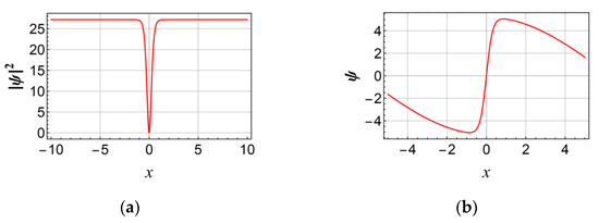
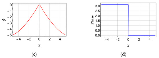
Figure 1.
Waveform plots of dark soliton for the (1+1)D RNLSE incorporating 3OD and 4OD dispersions with Kerr nonlinearity with the parameters , , , , . when for (a) modulus, (b) real part, (c) imaginary part, and (d) phase.
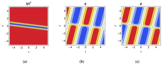
Figure 2.
Contour plots of dark soliton for (1+1)D RNLSE incorporating 3OD and 4OD dispersions with Kerr nonlinearity with the parameters , , , , , and under time diffusion for (a) modulus, (b) real part, and (c) imaginary part.
Subsequently, RNLSE incorporating 3OD and 4OD dispersions with Kerr nonlinearity is investigated in the (2+1)D case. The equation is expressed as:
By considering the self-similar method, the (2+1)D traveling wave ansatz can be expressed as:
where the is expressed in the following (2+1)D form:
where , , , , and are undetermined coefficients. We calculate the partial derivatives involved in Equation (22) and substitute them into Equation (22). Then, we separate the real and imaginary parts. The F-expansion method is reapplied to derive the expressions. Finally, by substituting the obtained expressions into Equation (20), the solution can be formulated as:
where , .
Figure 3 shows the waveform plots of the dark soliton solution of Equation (25) under appropriate coefficients and static conditions of , while Figure 4 shows corresponding contour plots.
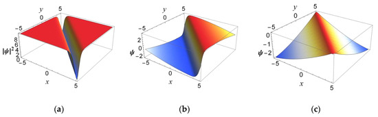
Figure 3.
Waveform plots of dark soliton for (2+1)D RNLSE incorporating 3OD and 4OD dispersions with Kerr nonlinearity with the parameters , , , , , , , and when for (a) modulus, (b) real part, and (c) imaginary part.
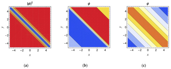
Figure 4.
Contour plots of dark soliton for (2+1)D RNLSE incorporating 3OD and 4OD dispersions with Kerr nonlinearity with the parameters , , , , , , , and when for (a) modulus, (b) real part, and (c) imaginary part.
4. Dark Soliton Solution for RNLSE with 3OD and 4OD Dispersions with PTs
In order to understand the RNLSE with 3OD and 4OD dispersions in depth, the (1+1)D RNLSE incorporating 3OD and 4OD dispersions with PTs is investigated. The equation is formulated as:
The parameters δ, λ, m, and μ shown in Equation (26) have the same definitions as those in Equation (2). Like the process for deriving the soliton solutions of (1+1)D RNLSE incorporating 3OD and 4OD dispersions without PTs shown in Section 3, the dark soliton solution for the model with PTs can be obtained as:
where . The detailed derivation process of Equation (27) is given in Appendix A. Figure 5 presents the dark soliton solution from Equation (27) under static conditions and appropriate coefficients, along with its contour plot under time diffusion. Moreover, by comparing the two (1+1)D models, which are the Equation (27) with PTs and Equation (21) without PTs, the amplitude coefficient C in Equation (27) explicitly depends on the inter-modal dispersion δ and self-steepening coefficient λ of PTs. In Equation (27), the term in the denominator in C replaces β in Equation (21), indicating that the self-steepening coefficient λ directly counteracts the Kerr nonlinearity β. On the other hand, the term before the variable t in Equation (27) gains an additional term δ compared with the Equation (21). This signifies that inter-modal dispersion δ directly alters the soliton propagation speed, independent of the dispersion coefficients α1, α2. This can also be clearly seen from the comparison of Figure 2a and Figure 5a; the deviation of the dark soliton in the x-direction is different within the same time range.
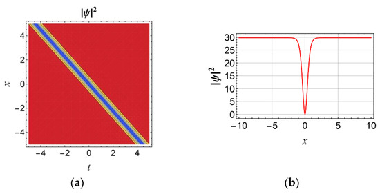
Figure 5.
Plots of dark soliton for the (1+1)D RNLSE incorporating 3OD and 4OD dispersions with Kerr nonlinearity in presence of PTs with parameters , , , , , , , and (a) when for modulus and (b) contour plot under time diffusion.
For the (2+1)D equation, the traveling wave ansatz from Equation (23) is applied and the F-expansion method is implemented following the standard procedure. Then, we derive the dark soliton solution for the (2+1)D RNLSE incorporating 3OD and 4OD dispersions and PTs, expressed as:
where , .
Figure 6 shows the dark soliton solution of Equation (28) under appropriate coefficients when t = 0. Combined with the comparison of the two (2+1)D models, which are Equation (28) with PTs and Equation (25) without PTs, this shows that, similar to the (1+1)D case, the amplitude coefficient D in Equation (25) incorporates PTs δ and λ. Moreover, the Kerr nonlinearity coefficient β is replaced by β+λk1 in the denominator of Equation (28). This shows that the self-steepening coefficient λ interacts with the wave number k1, modifying the effective nonlinearity governing the soliton’s amplitude. Additionally, the soliton propagation speed component gains an additive term δ. This inter-modal dispersion term δ directly increases the overall propagation speed in the (x+p2/p1y) direction, independent of the dispersion coefficients and wave numbers.
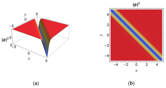
Figure 6.
Plots of dark soliton for in the (2+1)D RNLSE incorporating 3OD and 4OD dispersions with Kerr nonlinearity in the presence of PTs with parameters , , , , , , , , , and . (a) When for the modulus, (b) contour plot.
5. Modulation Instability for RNLSE with 3OD and 4OD Dispersions
Modulation instability (MI) is a fundamental phenomenon in nonlinear wave systems where a steady-state solution becomes unstable under small perturbations, leading to the exponential growth of sideband frequencies. MI analysis is implemented to investigate the (1+1)D RNLSE, incorporating 3OD and 4OD dispersions with Kerr nonlinearity and its PTs-included counterpart.
First, we give the steady-state solution of Equation (6). is defined as:
where represents the initial incident optical power. denotes the wave number and represents the frequency, all of which are real constants. By substituting Equation (29) into Equation (6), we obtain:
The perturbation is introduced and the perturbed solution is formulated as:
Then, the partial derivatives involved in Equation (31) can be formulated as:
By substituting Equations (31) and (32) into Equation (6) and applying linear stability analysis, we can derive:
where * denotes the complex conjugate. In addition, can be formulated as:
where and are perturbed power. and are the perturbed wave number and frequency, which are all real constants. By substituting Equation (34) into Equation (33) and organizing the coefficients and , we obtain:
The parameters in Equation (35) are calculated and expressed as:
When the determinant of the coefficient matrix is equal to zero, and in Equation (36) are non-zero solutions, that is:
The dispersion relation is obtained by solving the determinant and is expressed by:
For Equation (38), , is a real number, and Equation (38) is stable. Otherwise, when , is an imaginary number, and Equation (38) is unstable. By using the same approach to Equation (25), we derive its dispersion relation as follows:
where the expansion of is given by:
For Equation (39), if , is a real constant, and the Equation (39) is stable. If , is an imaginary number, and the Equation (39) becomes unstable. Besides, the MI gain spectrum quantifies the exponential growth rate imposed by the interplay of nonlinearity and dispersion on specific perturbation frequencies riding on an intense continuous-wave background. The MI gain spectrum quantifies the instability strength as a function of the perturbation wavenumber and can be derived as:
Figure 7 shows the MI gain spectrum of the RNLSE with and without PTs. It can be seen that the shapes of the gain spectra are similar for the two cases. This is because, based on Equation (40), the product of the high power of and the dispersion coefficient or , like , terms, dominate at large . It is suspected that these terms contribute to stabilizing the high-frequency perturbations so that the MI gain is small for the large absolute value of . Moreover, the peak of the MI gain spectrum for the RNLSE with PTs is lower than that without PTs, as shown in Figure 7. As shown in Equation (40), compared with the model without PTs, the value of can be reduced depending on the different values of parameters δ, λ, μ, which will compress the unstable regions and lead to a decrease in the peak gain. Qualitatively, the generation of MI mainly depends on a certain balance between nonlinear effects and dispersion effect [30]. If the perturbed parameter μ related to the high-order dispersion is a negative number, this means that the total dispersion of the model will be reduced. In this case, the peak gain will also decrease in order to reduce the nonlinear effect to make a new balance with the reduced dispersion.
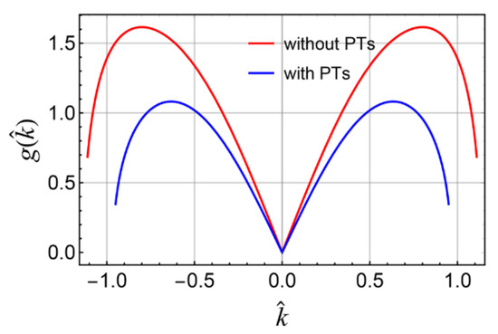
Figure 7.
MI gain spectrum when , , , , , , , , , .
6. Conclusions
In this study, the RNLSE model incorporating 3OD and 4OD dispersions with Kerr nonlinearity are investigated. We derive dark soliton solutions for both (1+1)D and (2+1)D cases using the F-expansion and self-similar methods, extending the analysis to the models with PTs. By comparing the (1+1)D and (2+1)D models and graphical results, it is found that the parameters δ and λ in PTs alter the soliton amplitude by modifying the Kerr nonlinearity coefficient β. Moreover, inter-modal dispersion δ induces a direct shift in the soliton propagation speed. MI analysis reveals significant suppression of the MI growth rate induced by PTs. The theoretical results provide a foundation for the research on solitons in systems governed by the RNLSE model and further experimental investigation.
Author Contributions
Conceptualization, W.Z. and Y.W. (Ying Wang); methodology, W.Z.; software, Z.W.; validation, Z.W., Y.W. (Yuan Wang) and Z.W.; formal analysis, Y.W. (Yuan Wang); investigation, W.Z.; resources, Y.W. (Ying Wang); data curation, W.Z.; writing—original draft preparation, W.Z.; writing—review and editing, Y.W. (Yuan Wang); visualization, Y.W. (Yuan Wang); supervision, Y.W. (Yuan Wang); project administration, Z.W. and Y.W. (Ying Wang); funding acquisition, Z.W. and Y.W. (Ying Wang). All authors have read and agreed to the published version of the manuscript.
Funding
This research was funded by National Natural Science Foundation of China, grant number 11547024 and National Natural Science Foundation of China, grant number 62301236.
Data Availability Statement
The original contributions presented in this study are included in the article. Further inquiries can be directed to the corresponding author(s).
Conflicts of Interest
The authors declare no conflict of interest.
Appendix A
This appendix gives the detailed derivation procedure of the (1+1)D RNLSE incorporating 3OD and 4OD dispersions with PTs. The equation is formulated as:
The parameters δ, λ, m, μ shown in Equation (A1) have the same definitions as those defined in Equation (2). Based on the previous steps, the traveling wave ansatz defined in Equation (7) is applied to the (1+1)D equation. Substituting the ansatz into Equation (A1), all partial derivatives involved in Equation (A1) can be expressed as:
Due to the integrability condition, m needs to be equal to 1 [31], which consequently leads to the following expression:
By substituting Equations (A2) and (A3) into Equation (A1) and subsequently separating the imaginary and real parts, we obtain:
Simultaneously, the F-expansion method from Equation (13) is applied. Substituting Equation (14) into Equation (A4), we can get the coefficients of each term:
By solving the system of equations in Equation (A5), we obtain:
Consequently, the exact solution can be expressed as:
where .
References
- Taylor, J.R. Optical Solitons-Theory and Experiment, 3rd ed.; Cambridge University Press: Cambridge, UK, 2004; pp. 1–14. [Google Scholar]
- Kumar, S.; Mohan, B. Lump, soliton, and interaction solutions to a generalized two-mode higher-order nonlinear evolution equation in plasma physics. Nonlinear Dyn. 2022, 110, 693–704. [Google Scholar] [CrossRef]
- Kudryashov, N.A. Mathematical model of propagation pulse in optical fiber with power nonlinearities. Optik 2020, 212, 164750. [Google Scholar] [CrossRef]
- Helal, M.A. Soliton solution of some nonlinear partial differential equations and its applications in fluid mechanics. Chaos Soliton Fract. 2002, 13, 1917–1929. [Google Scholar] [CrossRef]
- Tang, D.; Guo, J.; Song, Y.; Zhang, H.; Zhao, L.; Shen, D. Dark soliton fiber lasers. Opt. Express 2014, 22, 19831–19837. [Google Scholar] [CrossRef]
- Hasegawa, A.; Tappert, F. Transmission of stationary nonlinear optical pulses in dispersive dielectric fibers. I. Anomalous dispersion. Appl. Phys. Lett. 1973, 23, 142–144. [Google Scholar] [CrossRef]
- Hasegawa, A. Soliton-based optical communications: An overview. IEEE J. Sel. Top. Quant. 2000, 6, 1161–2000. [Google Scholar] [CrossRef]
- Kivshar, Y.S. Dark solitons in nonlinear optics. IEEE J. Quantum Elect. 1993, 29, 250–264. [Google Scholar] [CrossRef]
- Herr, T. Solitons and Dynamics of frequency Comb Formation in Optical Microresonators. Ph.D. Thesis, École Polytechnique Fédérale de Lausanne, Lausanne, Switzerland, 2013. [Google Scholar]
- Ray, S.S. Nonlinear Differential equations in Physics Novel Methods for Finding Solutions; Springer: Berlin/Heidelberg, Germany, 2020; pp. 1–2. [Google Scholar]
- Abbas Haider, J.; Alhuthali, A.M.S. Exploring novel applications of stochastic differential equations: Unraveling dynamics in plasma physics with the Tanh-Coth method. Results Phys. 2024, 60, 107684. [Google Scholar] [CrossRef]
- Peng, X.; Zhao, Y.-W. Data-driven solitons and parameter discovery to the (2+1)-dimensional NLSE in optical fiber communications. Nonlinear Dyn. 2023, 112, 1291–1306. [Google Scholar] [CrossRef]
- Akram, G.; Sadaf, M. Soliton solutions of the resonant nonlinear Schrödinger equation using modified auxiliary equation method with three different nonlinearities. Math. Comput. Simul. 2023, 206, 1–20. [Google Scholar] [CrossRef]
- Bulut, H.; Sulaiman, T.A. Optical solitons to the resonant nonlinear Schrödinger equation with both spatio-temporal and inter-modal dispersions under Kerr law nonlinearity. Optik 2018, 163, 49–55. [Google Scholar] [CrossRef]
- Rezazadeh, H.; Abazari, R. New optical solitons of conformable resonant nonlinear Schrödinger’s equation. Open Phys. 2020, 18, 761–769. [Google Scholar] [CrossRef]
- Biswas, A. Cubic–quartic optical solitons in Kerr and power law media. Optik 2017, 144, 357–362. [Google Scholar] [CrossRef]
- Bansal, A.; Biswas, A. Lie symmetry analysis for cubic–quartic nonlinear Schrödinger’s equation. Optik 2018, 169, 12–15. [Google Scholar] [CrossRef]
- Li, Y.; Kai, Y. Wave structures and the chaotic behaviors of the cubic-quartic nonlinear Schrödinger equation for parabolic law in birefringent fibers. Nonlinear Dyn. 2023, 111, 8701–8712. [Google Scholar] [CrossRef]
- Zahran, E.H.M.; Bekir, A. New private types for the cubic-quartic optical solitons in birefringent fibers in its four forms of nonlinear refractive index. Opt. Quantum Electron. 2021, 53, 680. [Google Scholar] [CrossRef]
- AlQahtani, S.A.; Alngar, M.E.M. Soliton solutions of perturbed NLSE-CQ model in polarization-preserving fibers with cubic–quintic–septic–nonic nonlinearities. J. Opt. 2023, 53, 3789–3796. [Google Scholar] [CrossRef]
- Ahmad, J. Novel resonant multi-soliton solutions of time fractional coupled nonlinear Schrödinger equation in optical fiber via an analytical method. Results Phys. 2023, 52, 106761. [Google Scholar] [CrossRef]
- Wang, Y.; Wang, W. Solitons in One-Dimensional Bose–Einstein Condensate with Higher-Order Interactions. Commun. Theor. Phys. 2017, 68, 623–626. [Google Scholar] [CrossRef]
- Wang, Y.; Cheng, Q. Sonic horizon dynamics for quantum systems with cubic-quintic-septic nonlinearity. AIP Adv. 2019, 9, 075206. [Google Scholar] [CrossRef]
- Fei, J.X.; Zheng, C.L. Exact projective excitations of a generalized (3+ 1)-dimensional gross-Pitaevskii system with varying parameters. Chin. J. Phys. 2013, 51, 200–208. [Google Scholar]
- Tariq, K.U.; Inc, M.; Kazmi, S.M.R. Modulation instability, stability analysis and soliton solutions to the resonance nonlinear Schrödinger model with Kerr law nonlinearity. Opt. Quantum Electron. 2023, 55, 838. [Google Scholar] [CrossRef]
- Gao, W.; Ismael, H.F. Optical Soliton Solutions of the Cubic-Quartic Nonlinear Schrödinger and Resonant Nonlinear Schrödinger equation with the Parabolic Law. Appl. Sci. 2019, 10, 219. [Google Scholar] [CrossRef]
- Wang, Y.; Zhou, Y. Exact soliton solutions of the generalized Gross-Pitaevskii equation based on expansion method. AIP Adv. 2014, 4, 067131. [Google Scholar] [CrossRef]
- Zhao, Y.; Chen, Y. Bright Soliton Solution of (1+1)-Dimensional Quantum System with Power-Law Dependent Nonlinearity. Adv. Math. Phys. 2019, 2019, 8264848. [Google Scholar] [CrossRef]
- Chen, C.; Gao, G. Dark soliton dynamics for quantum systems with higher-order dispersion and higher-order nonlinearity. Mod. Phys. Lett. B 2021, 35, 17. [Google Scholar] [CrossRef]
- Abdullaev, F.K.; Bouketir, A.; Messikh, A.; Umarov, B.A. Modulational instability and discrete breathers in the discrete cubic–quintic nonlinear Schrödinger equation. Phys. D Nonlinear Phenom. 2007, 232, 54–61. [Google Scholar] [CrossRef]
- Gepreel, K.A. Exact soliton solutions for nonlinear perturbed Schrödinger equations with nonlinear optical media. Appl. Sci. 2020, 10, 8929. [Google Scholar] [CrossRef]
Disclaimer/Publisher’s Note: The statements, opinions and data contained in all publications are solely those of the individual author(s) and contributor(s) and not of MDPI and/or the editor(s). MDPI and/or the editor(s) disclaim responsibility for any injury to people or property resulting from any ideas, methods, instructions or products referred to in the content. |
© 2025 by the authors. Licensee MDPI, Basel, Switzerland. This article is an open access article distributed under the terms and conditions of the Creative Commons Attribution (CC BY) license (https://creativecommons.org/licenses/by/4.0/).