A Distortion Image Correction Method for Wide-Angle Cameras Based on Track Visual Detection

Abstract

Regarding the distortion correction problem of large field of view wide-angle cameras commonly used in railway visual inspection systems, this paper proposes a novel online calibration method for non-specially made cooperative calibration objects. Based on the radial distortion divisor model, first, the spatial coordinates of natural spatial landmark points are constructed according to the known track gauge value between two parallel rails and the spacing value between sleepers. By using the image coordinate relationships corresponding to these spatial coordinates, the coordinates of the distortion center point are solved according to the radial distortion fundamental matrix. Then, a constraint equation is constructed based on the collinear constraint of vanishing points in railway images, and the Levenberg–Marquardt algorithm is used to found the radial distortion coefficients. Moreover, the distortion coefficients and the coordinates of the distortion center are re-optimized according to the least squares method (LSM) between points and the fitted straight line. Finally, based on the above, the distortion correction is carried out for the distorted railway images captured by the camera. The experimental results show that the above method can efficiently and accurately perform online distortion correction for large field of view wide-angle cameras used in railway inspection without the participation of specially made cooperative calibration objects. The whole method is simple and easy to implement, with high correction accuracy, and is suitable for the rapid distortion correction of camera images in railway online visual inspection.

1. Introduction

Given the current advantages of machine vision inspection in terms of speed, cost, and visualization [1,2,3], it has received extensive attention and research in the field of track equipment inspection [4,5]. With the aid of a wide-angle camera with a large field of view, it is possible to very quickly perform overview scanning of the railway equipment to be inspected and then detect potential local fault points from it. However, due to the serious distortion problems in the images captured by the wide-angle camera, how to efficiently and accurately calibrate the camera parameters of the wide-angle camera with a large field of view and correct the distorted images has become a crucial problem to be solved urgently [6,7].

In the domain of large field of view wide-angle-lens cameras, several calibration methods have been developed. Traditional calibration methods rely on calibration objects with known dimensions, such as checkerboards [8]. By capturing images of the calibration object from diverse angles and positions, the camera’s internal and external parameters can be calculated [9]. Active vision calibration methods, on the other hand, eliminate the need for calibration objects, but require the camera to operate under specific motion conditions. The camera parameters are deduced by analyzing the camera’s motion trajectory and image changes [10]. Self-calibration methods utilize natural geometric features within the images, such as vanishing points or parallel lines, and employ algorithms to compute the camera parameters [11]. Moreover, there are improved methods. In the context of large field of view camera calibration, non-precise calibration plates are adopted while considering the influence of lens distortion. The calibration is achieved through establishing the calibration plate coordinate system, capturing calibration plate images, data processing, and global optimization [12].

To accurately calibrate and correct the large-distortion cameras used in railway visual inspection, this paper is based on the radial distortion division model. First, the spatial coordinates of natural spatial landmark points are constructed according to the known track gauge value between two parallel rails and the spacing value between sleepers. By utilizing the relationship between these spatial coordinates and their corresponding image coordinates, the coordinates of the distortion center point are solved based on the radial distortion fundamental matrix. Then, a constraint equation is constructed according to the collinear constraint of vanishing points. Moreover, the distortion coefficients and the coordinates of the distortion center are re-optimized according to the principle of minimizing the deviation error between points and the fitted straight line. Finally, based on the above, the distortion correction is carried out for the distorted railway images captured by the camera. The experimental results show that the above method can efficiently and accurately perform online distortion correction for large field of view wide-angle cameras used in railway inspection without the participation of specially made cooperative calibration objects. The whole method is simple and easy to implement, with high correction accuracy, and is suitable for the rapid distortion correction of camera images in railway online visual inspection.

2. Camera Imaging Model

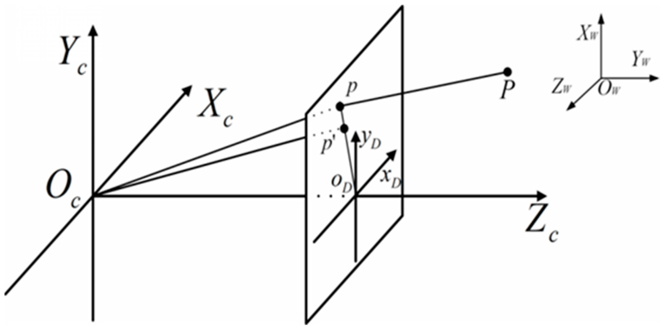
The process of projecting a point in a three-dimensional scene onto the two-dimensional image plane of a camera can be described using the pinhole imaging model [13], and the relevant demonstration is shown in Figure 1.

In Figure 1, O_W-X_WY_WZ_W represents the three-dimensional world coordinate system where the actual object points are located, O_D-X_DY_D represents the two-dimensional graphic coordinate system of the camera imaging plane, and O_C-X_CY_CZ_C represents the three-dimensional camera coordinate system. Among them, O_C and O_D represent the camera’s optical center and image center, respectively, and O_CO_D is the focal length f of the camera. The X_C axis and the Y_C axis are parallel to the x_D axis and the y_D axis of the image coordinate system, respectively, and the Z_C axis is perpendicular to the image plane. Under the ideal pinhole imaging model, using homogeneous coordinates uniformly, the projection of a spatial object point P(X_w, Y_w, Z_w, 1)^T on the image plane is the image point p(x_u, y_u, 1)^T. However, due to the existence of radial distortion in cameras, the actual imaging point will shift to the point p′(x_d, y_d, 1)^T.

2.1. Coordinate Transformation Relationship

A point P(X_w, Y_w, Z_w, 1)^T in the three-dimensional space is projected onto the two-dimensional image plane through pinhole imaging to form an image point p(x_u, y_u, 1)^T. The corresponding transformation relationship from the three-dimensional world coordinate system to the two-dimensional image coordinate system included in this process can be described using Equation (1):

$$\lambda p=A\left[\begin{array}{cc}R& t\end{array}\right]P,\mathrm{with} A=\left[\begin{array}{ccc}{f}_u& s& u_0\\ 0& f_v& v_0\\ 0& 0& 1\end{array}\right], R=\left[\begin{array}{ccc}{r}_1& r_2& r_3\end{array}\right]=\left[\begin{array}{ccc}{r}_{11}& r_{12}& r_{13}\\ r_{21}& r_{22}& r_{23}\\ r_{31}& r_{32}& r_{33}\end{array}\right], t=\left[\begin{array}{c}{t}_x\\ t_y\\ t_z\end{array}\right]$$

(1)

In the above equation, λ represents an arbitrary scale factor; (R, t) are called the external parameters, where R represents the rotation relationship between the two coordinate systems, r_i represents the i-th column of the rotation matrix R, and t represents the translation relationship between the two coordinate systems; A represents the camera’s internal parameter matrix, (u₀, v₀) are the principal point coordinates; f_u and f_v are the effective focal lengths (in pixels); and s is the parameter describing the skewness degree between the two image axes x and y.

Since a planar calibration model is adopted during the calibration process, it is assumed that the model plane Z_W = 0. Finally, Equation (1) can be transformed into the form represented using Equation (2):

$$\lambda \left[\begin{array}{c}{x}_u\\ y_u\\ 1\end{array}\right]=A\left[\begin{array}{cccc}{r}_1& r_2& r_3& t\end{array}\right]\left[\begin{array}{c}{X}_W\\ Y_W\\ 0\\ 1\end{array}\right]=A\left[\begin{array}{ccc}{r}_1& r_2& t\end{array}\right]\left[\begin{array}{c}{X}_W\\ Y_W\\ 1\end{array}\right]$$

(2)

Therefore, a homography matrix H can be used to relate the world coordinates of the landmark points to their image coordinates. The relationship between them is shown in Equation (3) as follows:

$$\lambda p=HP,with H=A\left[\begin{array}{ccc}{r}_1& r_2& t\end{array}\right]$$

(3)

2.2. Representation Method of Radial Distortion

Since there will be deviations during the processing and assembly of the camera lens, the camera imaging system will have corresponding imaging distortion. Regarding the camera distortion, Fitzgibbon proposed a division model (DM) to describe this distortion process [14], which can be expressed using Equation (4):

$$p-e={\displaystyle \frac{\left(p^{\prime }-e\right)}{1+k_1{r}_d^2+k_2{r}_d^4+\cdots }}$$

(4)

Among them, k₁ and k₂ are the radial distortion coefficients, e = (e_u0, e_v0, 1)^T represents the homography coordinates of the distortion center, and r_d is the pixel radius from the pixel point p′(x_d, y_d, 1)^T to the distortion center e(e_u0, e_v0, 1)^T.

Moreover, e can also be expressed as in Equation (5):

$$\left\{\begin{array}{c}{x}_u-e_{u0}={\displaystyle \frac{\left(x_d-e_{u0}\right)}{1+k_1{r}_d^2+k_2{r}_d^4+\cdots }}\\ y_u-e_{v0}={\displaystyle \frac{\left(y_d-e_{v0}\right)}{1+k_1{r}_d^2+k_2{r}_d^4+\cdots }}\end{array}\right.$$

(5)

3. Distortion Correction Method

The whole process of image distortion correction can roughly be divided into three steps. Firstly, the distortion center is accurately estimated using epipole constraints. Then, based on the radial distortion division model, the distortion coefficient is calculated using the vanishing point correspondence between the images formed by the parallel lines of the orbit. In the third step, the 3σ rule is used to screen and optimize the distortion parameters, and finally perform distortion image correction.

3.1. Estimation of Distortion Center

For the distorted images captured by the camera, most previous studies analyzed the images by taking the image center as the distortion center. However, some studies have found that due to the deviations during the processing and assembly of the lens, the distortion center will also deviate from the image center [15]. Therefore, the accurate solution of the distortion center is particularly crucial for the high-precision correction of distorted images.

In this paper, we adopt the method proposed in reference [16] to accurately solve the distortion center of the camera. For Equation (4), if we let $Ci=1+k_1{r}_{id}^2+k_2{r}_{id}^4+\cdots$, then Equation (4) can be rewritten as Equation (6):

$${p_i}^{\prime }=e+C_i\left(p_i-e\right)$$

(6)

For Equation (6), multiply both sides of the equation on the left by [p_i′]^T[e]_× ([e]_×, which represents the 3 × 3 skew-symmetric matrix of [e], $\left({\left[e\right]}_{\times }=\left[\begin{array}{ccc}0& -1& e_{v0}\\ 1& 0& -e_{u0}\\ -e_{v0}& e_{u0}& 0\end{array}\right]\right)$. According to p_i = HP_i, C_i must not be equal to 0 (a value of 0 would imply no distortion in the image, which is impossible), and Equation (7) can be obtained:

$$0=C_i{\left[{p_i}^{\prime }\right]}^T\left({\left[e\right]}_{\times }H\right)P_i={\left[{p_i}^{\prime }\right]}^T\left({\left[e\right]}_{\times }H\right)P$$

(7)

By writing F_r = [e]_×H, which is called the radial distortion fundamental matrix, Equation (7) can be written as Equation (8):

$${\left[{p_i}^{\prime }\right]}^T{F}_r{P}_i=0$$

(8)

If a series of corresponding relationships between three-dimensional coordinate points and image points are known (the number of corresponding points is ≥8), the distortion center can be extracted through the left epipole of the fundamental matrix F_r [17], and the relevant relationship can be expressed using Equation (9):

$$e^T{F}_r=e^T{\left[e\right]}_{\times }H=0$$

(9)

3.2. Estimation of Distortion Parameters

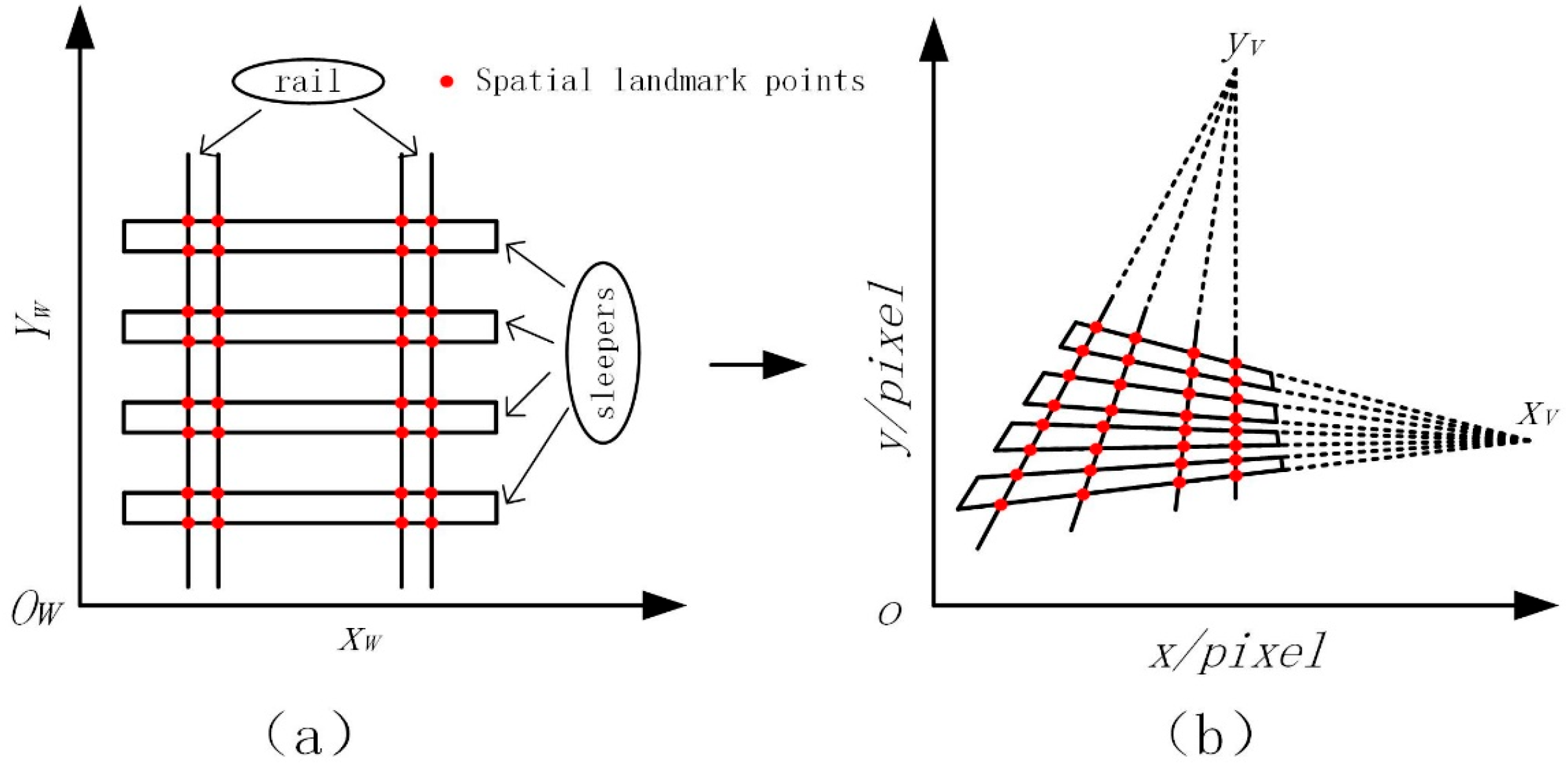
In the ideal pinhole imaging model, if there are parallel straight lines in space and these straight lines are not parallel to the image plane, without considering lens distortion, the extended lines of the projections of these parallel straight lines on the image plane will intersect at a point, and this point is the vanishing point corresponding to the parallel straight lines in space [18]. For the straight railway tracks, there are parallel relationships between sleepers and between the two rails. After the projection imaging of these parallel straight lines, there will be corresponding vanishing points. The imaging situation of the vanishing points in the railway track images is shown in Figure 2.

Figure 2a is a schematic diagram of the railway track on the spatial plane. For the sake of convenience, it is assumed that Z_w = 0. Figure 2b is a schematic diagram of the railway track after non-parallel overhead perspective projection. X_V and Y_V are the vanishing points corresponding to the horizontal and vertical directions of the track plane, respectively.

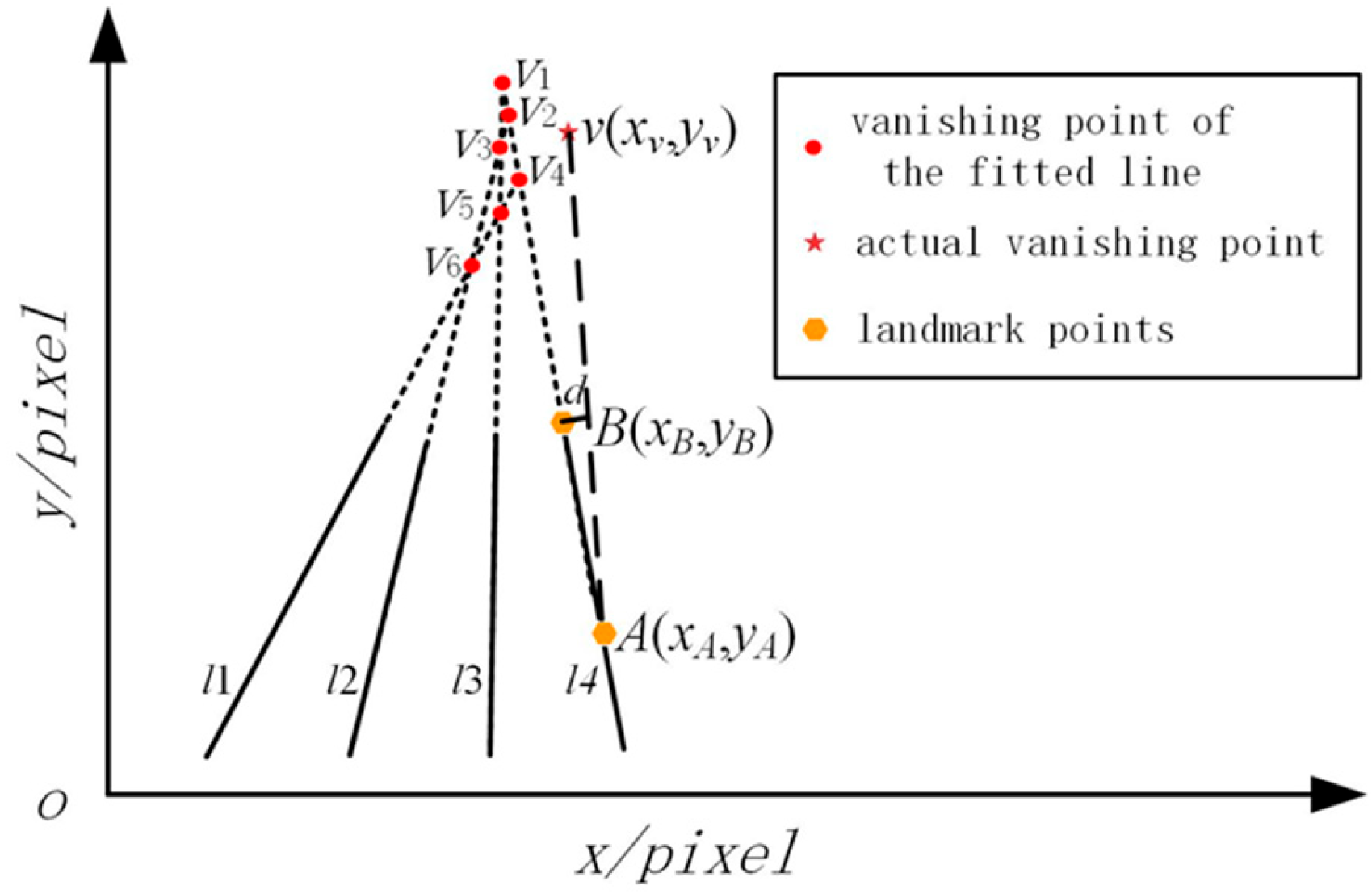
In the ideal undistorted case, the projected vanishing points of parallel line clusters in space should intersect at the same point. However, due to the influence of distortion, the vanishing points of these parallel line clusters after line fitting may exhibit multiple points. Therefore, the distortion coefficients of the distorted image can be solved based on the collinearity constraint between the vanishing points. The situation of the vanishing points formed by the projected distortion between the straight lines of parallel railway rails is shown in Figure 3.

As shown in Figure 3, four spatial parallel lines, l₁, l₂, l₃, and l_4, between railway rails are selected. The intersection points (i.e., vanishing points) formed by each pair of their projected lines are v₁, v₂, v₃, v₄, v₅, and v₆. Assume that the actual vanishing point coordinates of parallel lines in this direction under no camera distortion are v(x_v, y_v). Take any two landmark points, A(x_A, y_A) and B(x_B, y_B) on line l₄, and the mathematical expression of the line l_Av connecting points A and v can be represented using Equation (10):

$$y={\displaystyle \frac{y_v-y_A}{x_v-x_A}}x+y_A-{\displaystyle \frac{y_v-y_A}{x_v-x_A}}{x}_A$$

(10)

At this point, the distance between point B and the line l_Av can be expressed using Equation (11):

$$\left\{\begin{array}{l}d={\displaystyle \frac{\left|\left(x_B-x_A\right)\left(y_v-y_A\right)-\left(y_B-y_A\right)\left(x_v-x_A\right)\right|}{S_{Av}}}\equiv 0\hfill \\ S_{Av}=\sqrt{{\left(x_v-x_A\right)}^2+{\left(y_v-y_A\right)}^2}\hfill \end{array}\right.$$

(11)

In the equation, S_Av represents the length of the line segment Av. If there is no distortion in the camera, the three points A, B, and v will lie on the same straight line in the image plane, and the distance d will be zero at this time. Suppose the pixel coordinates of the projection points formed by points A and B in the distorted image are (x_A′, y_A′) and (x_B′, y_B′), respectively, and r_A′ and r_B′ are the distortion radii from the distorted points (x_A′, y_A′) and (x_B′, y_B′) to the distortion center e(e_u0, e_v0). If there are j = 1, 2, …, m straight lines, and each line has i = 1, 2, …, n pairs of landmark points, the coordinates of the ideal vanishing point formed by these parallel lines are denoted as v(x_v, y_v). Using a second-order radial distortion model, substituting Equation (10) into Equation (11) yields the distance from point B′ to the line l_A′v, as shown in Equation (12):

$$\left\{\begin{array}{l}{F}_{ij}=\left|{\displaystyle \frac{\left[\left(\frac{x_{B^{\prime }}-e_{u0}}{c_B}-\frac{x_{A^{\prime }}-e_{u0}}{c_A}\right)\left(y_v-\frac{y_{A^{\prime }}-e_{v0}}{c_A}-e_{v0}\right)-\left(\frac{y_{B^{\prime }}-e_{v0}}{c_B}-\frac{y_{A^{\prime }}-e_{v0}}{c_A}\right)\left(x_v-\frac{x_{A^{\prime }}-e_{u0}}{c_A}-e_{u0}\right)\right]}{\sqrt{{\left(x_v-\left(\frac{x_{A^{\prime }}-e_{u0}}{c_A}+e_{u0}\right)\right)}^2+{\left(y_v-\left(\frac{y_{A^{\prime }}-e_{v0}}{c_A}+e_{v0}\right)\right)}^2}}}\right|\hfill \\ \begin{array}{l}{r}_{A^{\prime }}=\sqrt{{\left(x_{A^{\prime }}-e_{u0}\right)}^2+{\left(y_{A^{\prime }}-e_{v0}\right)}^2},r_{B^{\prime }}=\sqrt{{\left(x_{B^{\prime }}-e_{u0}\right)}^2+{\left(y_{B^{\prime }}-e_{v0}\right)}^2}\\ c_A=1+k_1{\left(r_{A^{\prime }}\right)}^2+k_2{\left(r_{A^{\prime }}\right)}^4\\ c_B=1+k_1{\left(r_{B^{\prime }}\right)}^2+k_2{\left(r_{B^{\prime }}\right)}^4\end{array}\hfill \end{array}\right.$$

(12)

The value of F_ij should be close to 0. Therefore, the objective function can be constructed as shown in Equation (13):

$$F={\displaystyle \sum _{j=1}^m{\displaystyle \sum _{i=1}^n{F}_{ij}}}$$

(13)

Equation (13) is a nonlinear equation involving four parameters: x_v, y_v, k₁, and k₂. The distortion center e(e_u0, e_v0) has been obtained through previous calculations. At this stage, the intersection point (x_v, y_v) of any two lines and k₁ = k₂ = 0 are selected as the initial iteration values for parameter solving. The Levenberg–Marquardt algorithm is then used to iteratively optimize this equation. After iterative optimization, the numerical solutions for the four parameters (x_v, y_v, k₁, and k₂) can be obtained [19].

3.3. Optimization Using the 3σ Rule

After solving for the image distortion center e and distortion parameters k₁ and k₂, distortion correction can be performed on the railway distorted images captured by the camera. However, due to various random interferences in the image acquisition process and errors in the image landmark extraction method, not all acquired landmark points are highly accurate, and some even contain gross errors. If all landmark points are involved in the correction, it will inevitably lead to large correction errors. Therefore, it is necessary to screen and optimize the landmark points to obtain optimal parameters.

The 3σ rule can be used to eliminate bad data points in a set of data points containing random errors [20]. The process is to first calculate and process the data to obtain the standard deviation, and then determine an interval according to a certain probability. It is considered that any error exceeding this interval is a gross error, and the corresponding data can be eliminated.

A set of independent data {x₁, x₂, …, x_n} is obtained through equal-precision measurements. Calculate their arithmetic mean x and the residual errors v_i = x_i − x (i = 1, 2, …, n), and then calculate the standard deviation σ. If the residual error v_b (1 ≤ b ≤ n) of a certain measurement value x_b satisfies Equation (14),

$$\left|v_b\right|=\left|x_b-x\right|>3\sigma$$

(14)

Then x_b is considered a bad value containing a gross error, and should be eliminated.

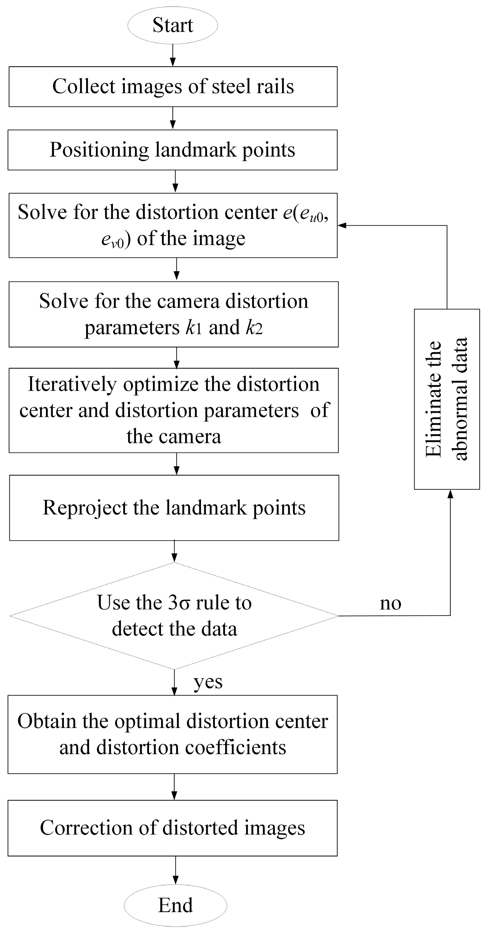
Therefore, after calculating the distortion center e and distortion parameters k₁ and k₂, the first step is to perform distortion correction on all landmark points involved in parameter calculation to obtain their corrected image positions. Next, calculate the distance between each landmark point and its corresponding fitted line, and then use the 3σ rule to filter out bad points with excessively large distances. After removing these identified bad points, re-calculate the correction parameters. Repeat the above screening process until all landmark points satisfy the 3σ rule. The final obtained distortion center e and distortion parameters k₁ and k₂ are the optimal parameters. The whole parameter solution process is shown in Figure 4.

4. Experiments

In order to verify the reliability of the distortion correction method proposed in this paper, this method is applied to perform distortion correction on some computer-simulated image data with large distortion and actual distorted image data. By conducting a distance error analysis between the corrected coordinates of the landmark points obtained through this method and the coordinates set in the simulation, and simultaneously comparing it with some other distortion correction methods, the correction accuracy of this method is tested. In addition, the correction effect of the method in this paper is practically verified by performing distortion correction on the distorted railway track images captured by the large field of view wide-angle camera.

4.1. Computer Simulation Images

The imaging model of the camera is simulated by a computer to obtain standard distortion-free image data points. The image size of the simulated camera set here is 1280 × 1024 pixels, and the principal point (u₀, v₀) of the image is located at the pixel coordinates (640, 512). The normalized focal lengths f_u and f_u are 850 and 850, respectively, and the skew parameter s is set to 0. The distortion center e(e_u0, e_v0) of the image is set to be in the same position as the coordinates of the principal point. The radial distortion coefficients are k₁ = −6 × 10⁻⁷ pixel⁻² and k₂ = −2 × 10⁻¹³ pixel⁻⁴.

For railway tracks, taking the 60 kg/m standard rail as a reference, the track gauge is set to 1435 mm, the rail base width is 150 mm, the sleeper width is 120 mm, and the spacing between sleepers is 250 mm. Four intersection points formed by the cross between the rail base and the sleepers are defined as a set of marker points, creating a simulated track image with two parallel rails and three parallel, equally spaced sleepers. To simulate track images at different projection angles, three sets of rotation matrices R are selected: R₁ = [20, 0, 0]^T, R₂ = [15, 5, 0]^T, and R₃ = [20, 5, 5]^T; and three sets of translation coordinates T: T₁ = [−100, −60, 220]^T, T₂ = [100, 60, 220]^T, and T₃ = [−100, −60, −220]^T. Additionally, Gaussian noise with a mean of 0 and a standard deviation of 0.5 is added to the simulated images to better approximate the actual imaging process. 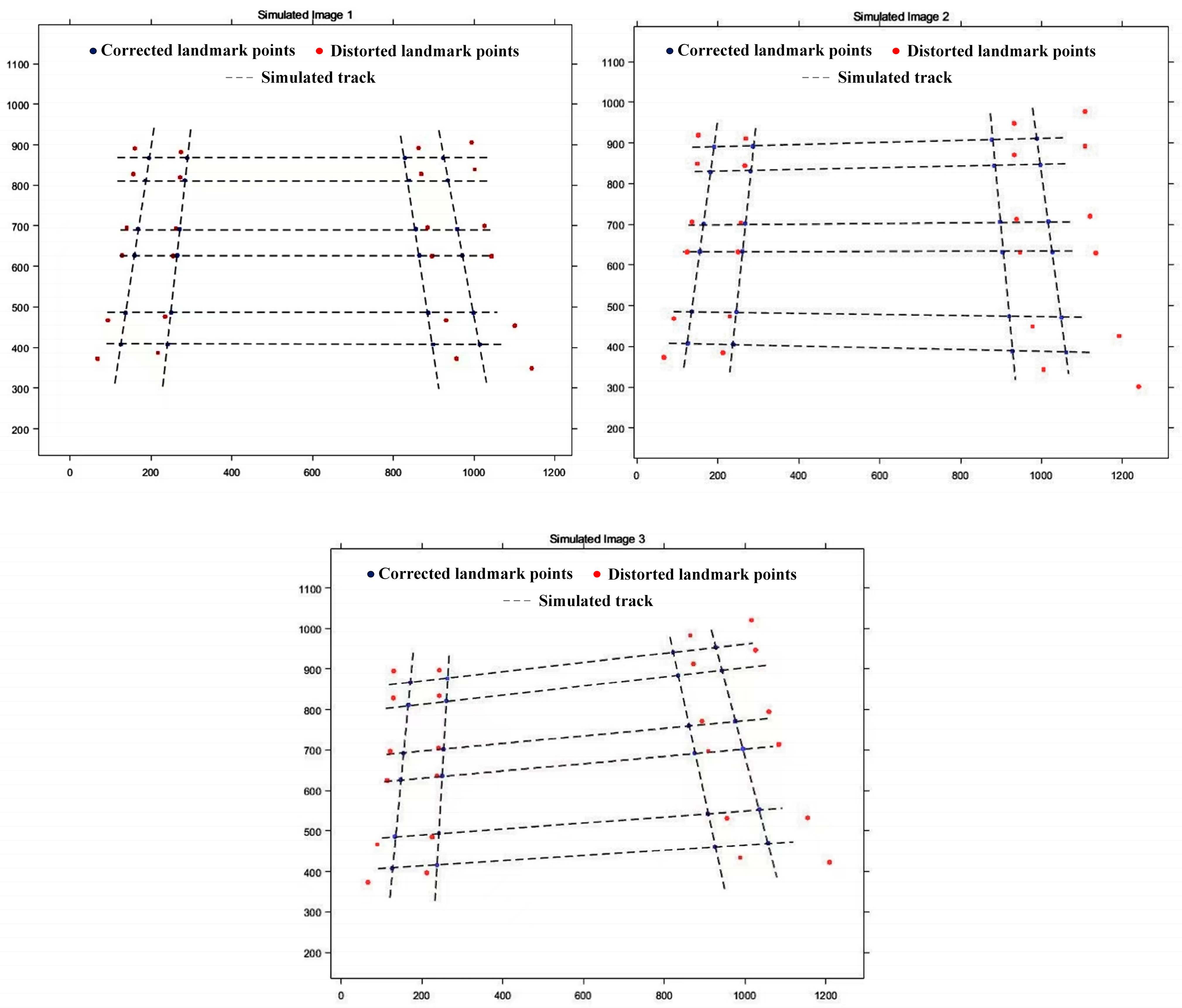Figure 5 shows the relevant simulated images and their correction effects, where the black dashed lines represent the simulated track, with the intersection points of horizontal and vertical lines being undistorted marker points; red marker points indicate distorted marker points after simulation; and blue marker points represent marker points corrected using the method in this paper.

From Figure 5, it can be observed that the corrected marker positions are very close to the simulated marker positions. To verify the effectiveness of the method in this paper, the distortion centers and distortion parameters of three simulated test images were solved using both the method proposed herein and the method in Reference [16]. Additionally, the mean squared re-projection error (E_msre) after correction for the three simulated test images was calculated, with the calculation equation for E_msre shown in Equation (15):

$$E_{msre}=\sqrt{{\displaystyle \frac{1}{n}}{\displaystyle \sum _{i=1}^n\left[{\left(x_{id}-x_{iu}\right)}^2+{\left(y_{id}-y_{iu}\right)}^2\right]}}$$

(15)

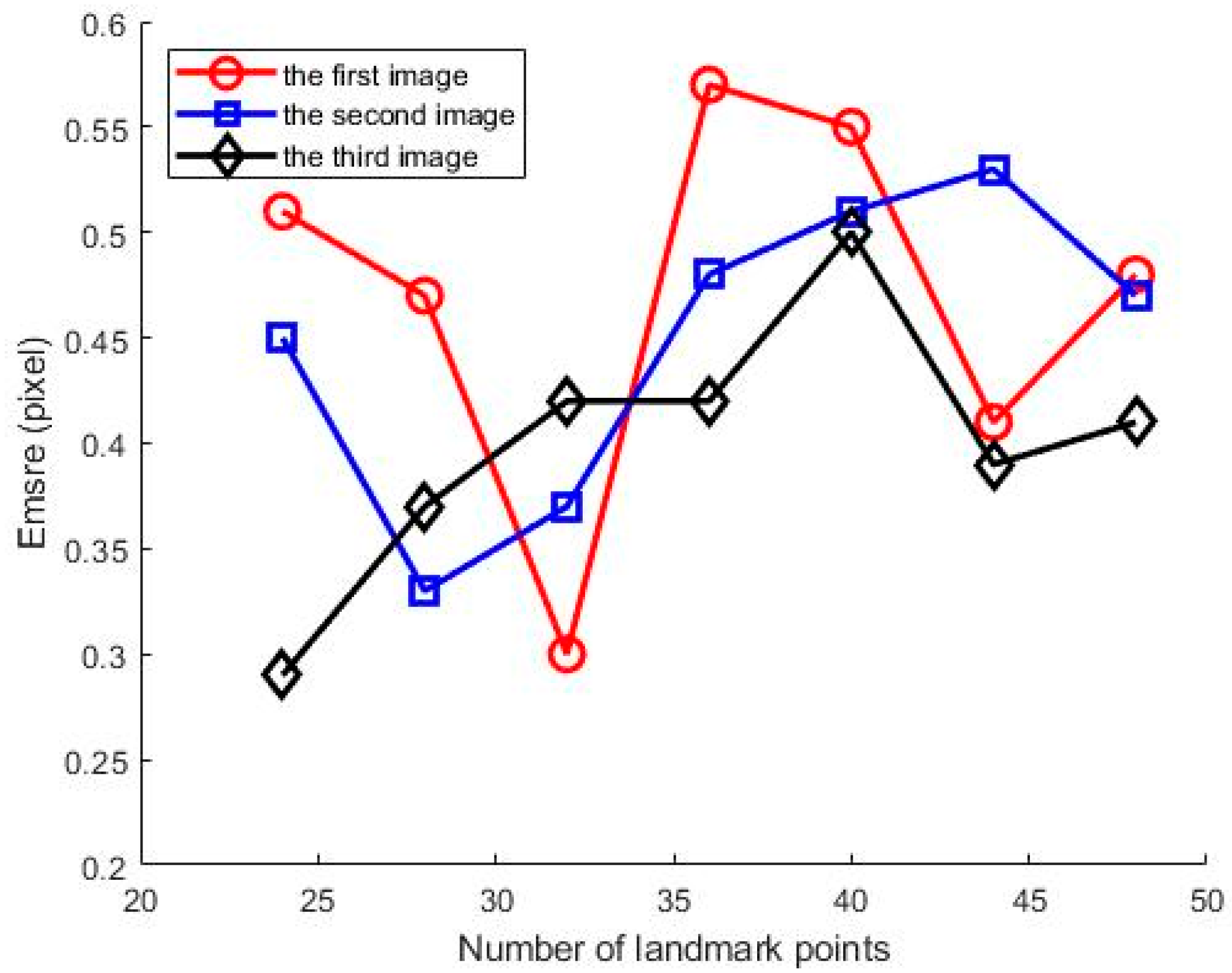
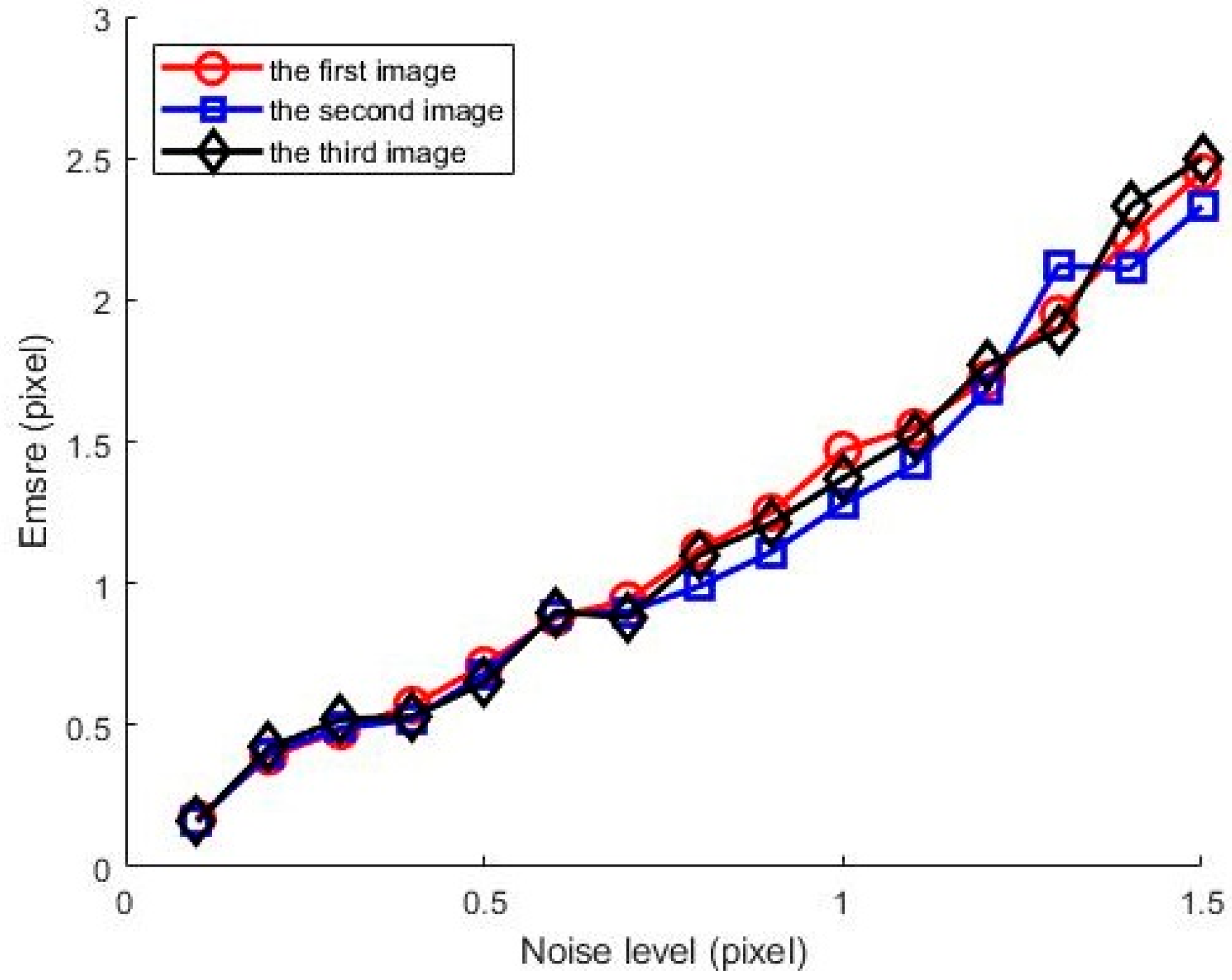
In order to statistically analyze the sensitivity impact of the number of participating landmark points and data noise on correction accuracy, we separately counted the correction accuracy in three simulated images under two scenarios: the number of landmark points ranging from 24 to 48, with an interval of 4, and noise levels from 0.1 to 1.5 pixels, with an interval of 0.1 pixel. For each scenario, 20 independent trials were conducted, and the average values were taken. The results are shown in Figure 6 and Figure 7, respectively.

From Figure 6, it can be seen that the number of landmark points involved in calibration does not have a significant impact on E_msre, with an accuracy of 0.4 ± 0.2 pixels. This indicates that the number of landmark points has little effect on calibration accuracy, while the coordinate extraction accuracy of landmark points has a greater impact on calibration accuracy. On the other hand, it can be observed from Figure 7 that the E_msre increases linearly with the noise level.

The comparison results of the distortion correction for the three simulated images are shown in Table 1.

Table 1. Correction results of simulated images.

	Parameter	k1	k2	eu0	eu0	Emsre
Method
Simulated image		−6 × 10−7 pixel−2	−2 × 10−13 pixel−4	640	512	--
Reference [16]	Image 1	−6.17 × 10−7 pixel−2	−1.92 × 10−13 pixel−4	641.53	511.68	0.1769
	Image 2	−6.13 × 10−7 pixel−2	−2.02 × 10−13 pixel−4	639.88	511.74	0.1886
	Image 3	−5.94 × 10−7 pixel−2	−2.02 × 10−13 pixel−4	639.27	511.75	0.1771
Proposed	Image 1	−6.20 × 10−7 pixel−2	−1.89 × 10−13 pixel−4	640.88	512.09	0.1882
	Image 2	−6.20 × 10−7 pixel−2	−2.11 × 10−13 pixel−4	639.67	512.43	0.1767
	Image 3	−5.87 × 10−7 pixel−2	−1.95 × 10−13 pixel−4	640.79	511.73	0.1759

Table 1. Correction results of simulated images.

	Parameter	k1	k2	eu0	eu0	Emsre
Method
Simulated image		−6 × 10−7 pixel−2	−2 × 10−13 pixel−4	640	512	--
Reference [16]	Image 1	−6.17 × 10−7 pixel−2	−1.92 × 10−13 pixel−4	641.53	511.68	0.1769
	Image 2	−6.13 × 10−7 pixel−2	−2.02 × 10−13 pixel−4	639.88	511.74	0.1886
	Image 3	−5.94 × 10−7 pixel−2	−2.02 × 10−13 pixel−4	639.27	511.75	0.1771
Proposed	Image 1	−6.20 × 10−7 pixel−2	−1.89 × 10−13 pixel−4	640.88	512.09	0.1882
	Image 2	−6.20 × 10−7 pixel−2	−2.11 × 10−13 pixel−4	639.67	512.43	0.1767
	Image 3	−5.87 × 10−7 pixel−2	−1.95 × 10−13 pixel−4	640.79	511.73	0.1759

It can be found from Figure 5 and Table 1 that the correction method in this paper can effectively correct the distorted track images, and that the correction error is roughly comparable to that of the method in Reference [16].

4.2. Actual Images

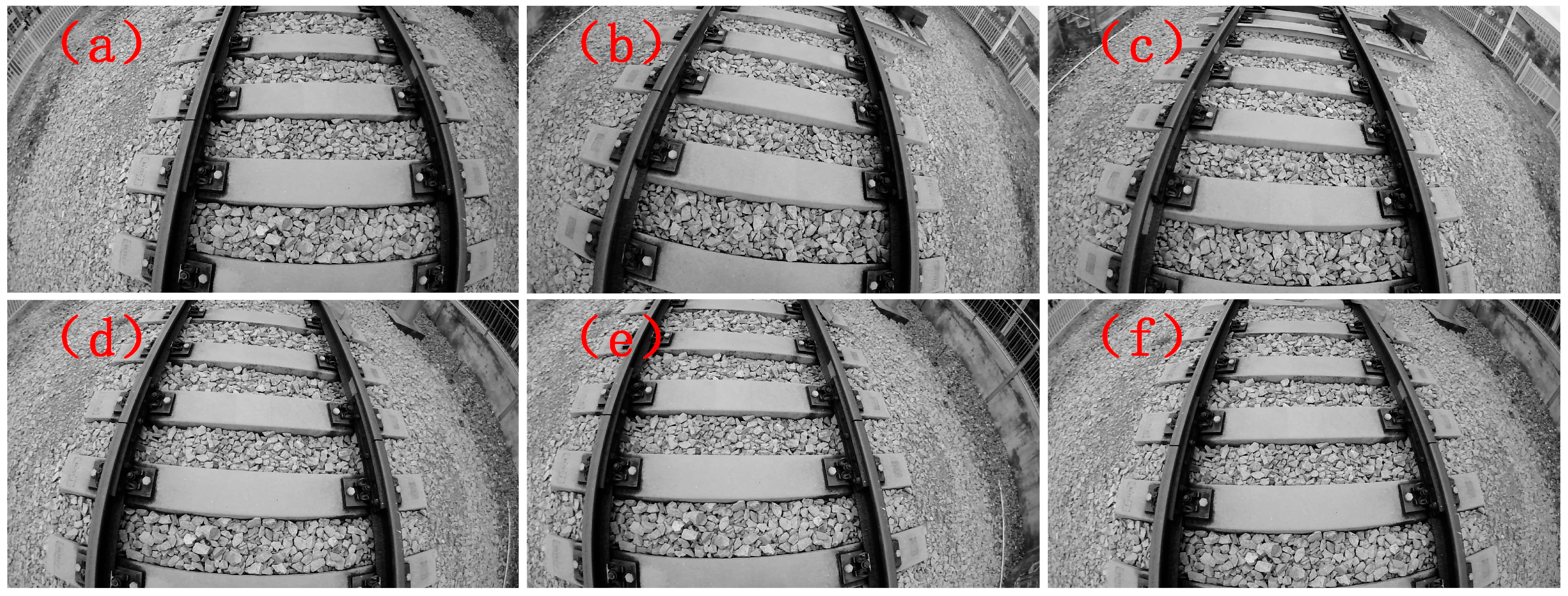
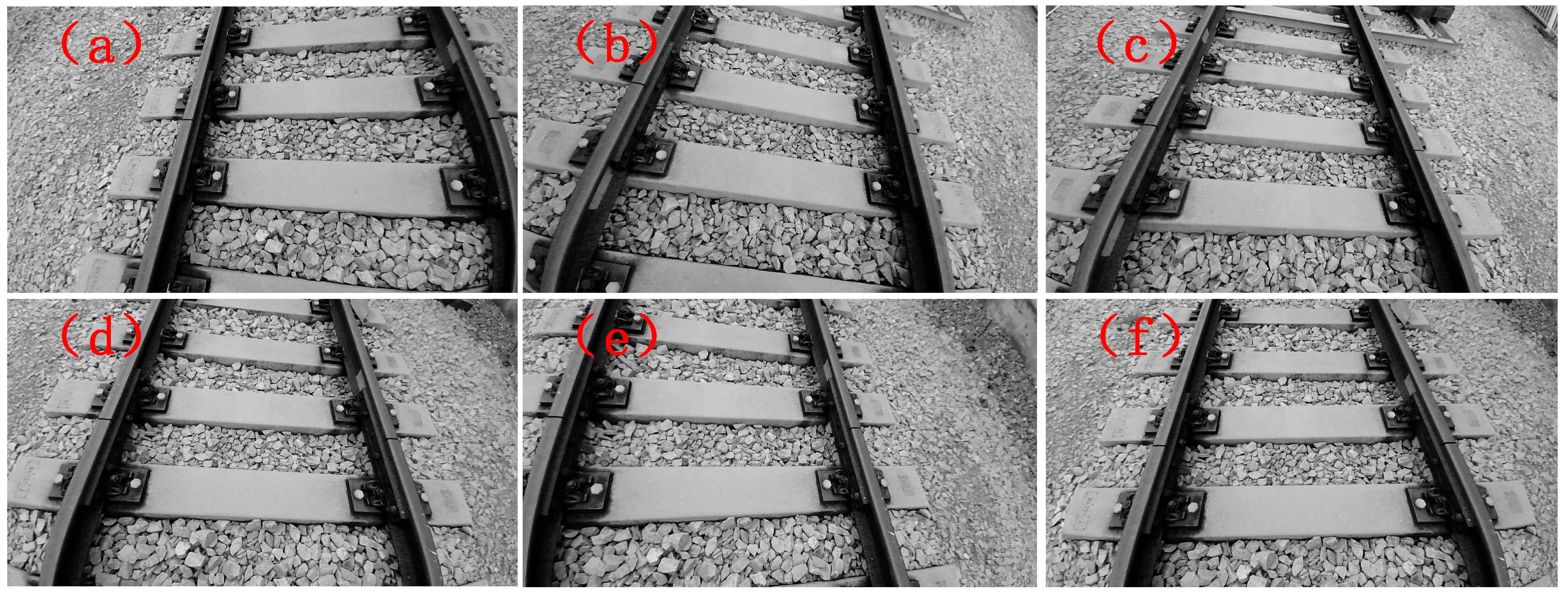
To further verify the effectiveness of the proposed method in practical applications, a field correction experiment was conducted using an HBVCAM-4M2214HD camera (Huiber Vision Technology Co., Ltd., Shenzhen, China) equipped with a 3.6 mm lens. Six distorted track images at different angles were collected, and distortion correction was performed on these images using the method in this paper, the method in Reference [16], and Zhang’s calibration method [21]. The relevant distorted images are shown in Figure 8.

The images corrected using the method in this paper are shown in Figure 9.

The average values of the correction effects of the three methods were statistically analyzed, and the results are shown in Table 2. It should be noted that, on the one hand, Zhang’s calibration method does not consider the distortion center e(e_u0, e_v0), while the method in this paper and the method in Reference [16] calculate the distortion center. On the other hand, Zhang’s calibration method uses a polynomial model to describe lens distortion, whereas the methods in this paper and Reference [16] are based on the division model, resulting in different expressions for the obtained distortion coefficients.

Table 2. Correction results of actual images.

	Parameter	k1	k2	eu0	ev0	Emsre
Method
Zhang’s calibration		−0.33 mm−2	0.11 mm−4	--	--	0.1775
Reference [16]		−4.77 × 10−7 pixel−2	−1.64 × 10−13 pixel−4	924.03	521.49	0.1791
Proposed		−4.88 × 10−7 pixel−2	−1.71 × 10−13 pixel−4	925.10	522.56	0.1777

Table 2. Correction results of actual images.

	Parameter	k1	k2	eu0	ev0	Emsre
Method
Zhang’s calibration		−0.33 mm−2	0.11 mm−4	--	--	0.1775
Reference [16]		−4.77 × 10−7 pixel−2	−1.64 × 10−13 pixel−4	924.03	521.49	0.1791
Proposed		−4.88 × 10−7 pixel−2	−1.71 × 10−13 pixel−4	925.10	522.56	0.1777

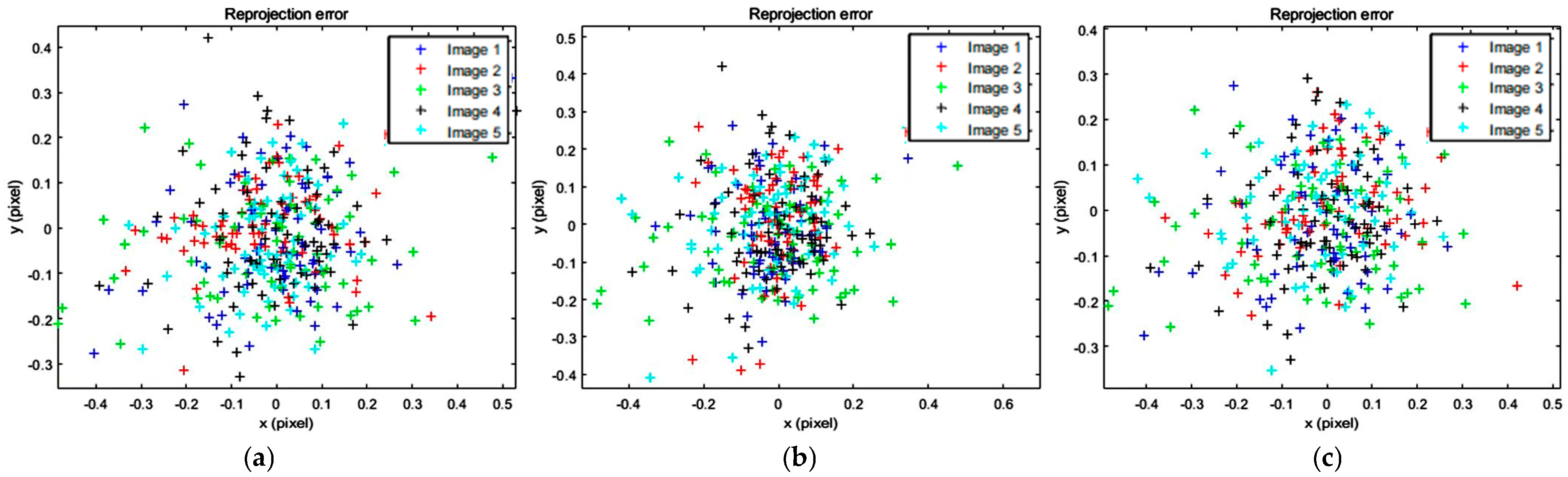
The re-projection error distribution of each landmark point in the five images after being corrected using three methods is shown in Figure 10.

It can be seen from the calculations in Table 2 that for the five test images, the average value of the mean square re-projection error after correction using the method in this paper is reduced by 0.0014 pixels compared with that of the method in Reference [16], which is equivalent to an improvement of 0.78% in the accuracy of the calibration error. It can also be found from Figure 10 that compared with Zhang’s calibration method and the calibration method in Reference [16], the distribution points of the correction errors obtained using the method in this paper are more concentrated near the central point. This indicates that the method in this paper can avoid the off-center effect caused by individual error data points and can better serve subsequent image processing.

From the correction experimental results of both simulated image data and actual image data, it can be seen that the method proposed in this paper can accurately perform distortion correction on the track distortion images captured by wide-angle cameras with large fields of view, and can serve well the application scenarios of track visual inspection.

5. Conclusions

In this paper, a novel online distortion correction method for railway inspection cameras is proposed. This method overcomes the reliance of traditional approaches on specially made calibration objects. It leverages natural railway landmarks—track gauges and sleeper spacings—decoupling distortion center and radial coefficient estimation for more stable results. The distortion center is accurately solved via the radial distortion fundamental matrix, critical for correction precision. Experimental results on simulated and real railway data validate the method’s robustness and effectiveness. It avoids complex early nonlinear optimization, using the Levenberg–Marquardt algorithm and least squares method for efficient parameter estimation and refinement. Without artificial calibration markers, the method simplifies workflows while maintaining high accuracy, adapting well to dynamic railway environments. This provides a practical solution for real-time distortion correction in railway camera systems, enhancing the reliability of visual inspection data for railway infrastructure monitoring.

6. Discussion

For the detection of railway track diseases, wide-angle cameras with large fields of view can be used to quickly acquire, collect, and analyze image information. However, for captured images with significant distortion, targeted methods are required for high-precision distortion correction of the camera. Without the use of special calibration objects, this paper considers the spatial characteristics of railway track distribution. First, the distortion center and distortion parameters are obtained based on the division model of radial distortion. Then, marker points with gross errors are eliminated according to the 3σ criterion, and parameter calculation is performed again. This process is repeated until no marker points with gross errors participate in the correction, ultimately obtaining the optimal correction parameters. Compared with Zhang’s calibration method, this paper separately considers and calibrates the camera’s distortion center. Additionally, since the entire calibration process is decoupled, it can effectively avoid the mutual influence of various parameters during calibration. In follow-up work, image analysis of the railway track’s visual measurement system can be considered based on this foundation.

References

- Zhu, G.; Li, Y.; Zhang, S.; Duan, X.; Huang, Z.; Yao, Z.; Wang, R.; Wang, Z. Neural Networks with Linear Adaptive Batch Normalization and Swarm Intelligence Calibration for Real-Time Gaze Estimation on Smartphones. Int. J. Intell. Syst. 2024, 2024, 2644725. [Google Scholar] [CrossRef]
- Huang, J. Automated Logistics Packaging Inspection Based on Deep Learning and Computer Vision: A Two-Dimensional Flow Model Approach. Trait. Signal 2025, 42, 933–941. [Google Scholar] [CrossRef]
- Park, J.S.; Park, H.S. Automated reconstruction model of a cross-sectional drawing from stereo photographs based on deep learning. Comput. Aided Civ. Infrastruct. Eng. 2024, 39, 383–405. [Google Scholar] [CrossRef]
- Cui, W.; Liu, W.; Guo, R.; Wan, D.; Yu, X.; Ding, L. Geometrical quality inspection in 3D concrete printing using AI-assisted computer vision. Mater. Struct. 2025, 58, 68. [Google Scholar] [CrossRef]
- Chen, C.; Qin, H.; Qin, Y.; Bai, Y. Real-Time Railway Obstacle Detection Based on Multitask Perception Learning. IEEE Trans. Intell. Transp. Syst. 2025, 26, 7142–7155. [Google Scholar] [CrossRef]
- Teague, S.; Chahl, J. Bootstrap geometric ground calibration method for wide angle star sensors. J. Opt. Soc. Am. A Opt. Image Sci. Vis. 2024, 41, 654–663. [Google Scholar] [CrossRef] [PubMed]
- Lin, H.Y.; Li, Y.Q.; Lin, D.T. System Implementation of Multiple License Plate Detection and Correction on Wide-Angle Images Using an Instance Segmentation Network Model. IEEE Trans. Consum. Electron. 2024, 70, 4425–4434. [Google Scholar] [CrossRef]
- Gennery, D.B. Generalized Camera Calibration Including Fish-Eye Lenses. Int. J. Comput. Vis. 2006, 68, 239–266. [Google Scholar] [CrossRef]
- Wang, Y.; Ye, F.; Chen, X.; Xi, J. Universal underwater camera calibration method based on a forward multilayer refractive model. Meas. Sci. Technol. 2025, 36, 035005. [Google Scholar] [CrossRef]
- Zhang, Y.; Wang, Y.; Wu, T.; Yang, J.; An, W. Fixed Relative Pose Prior for Camera Array Self-Calibration. IEEE Trans. Circuits Syst. Video Technol. 2025, 35, 981–985. [Google Scholar] [CrossRef]
- Zhao, Y.; Zhao, L.; Yang, F.; Li, W.; Sun, Y. Extrinsic Calibration of High Resolution LiDAR and Camera Based on Vanishing Points. IEEE Trans. Instrum. Meas. 2024, 73, 8506712. [Google Scholar] [CrossRef]
- Datta, A.; Kim, J.S.; Kanade, T. Accurate Camera Calibration using Iterative Refinement of Control Points. In Proceedings of the 2009 IEEE 12th International Conference on Computer Vision Workshops (ICCV Workshops), Kyoto, Japan, 27 September–4 October 2009. [Google Scholar] [CrossRef]
- Feng, B.; Liu, Z.; Zhang, H.; Fan, H. Research on the Measurement System and Remote Calibration Technology of a Dual Linear Array Camera. Meas. Sci. Rev. 2024, 24, 105–112. [Google Scholar] [CrossRef]
- Fitzgibbon, A.W. Simultaneous linear estimation of multiple view geometry and lens distortion. In Proceedings of the 2001 IEEE Computer Society Conference on Computer Vision and Pattern Recognition (CVPR 2001), Kauai, HI, USA, 8–14 December 2001; Volume 1, pp. I-125–I-132. [Google Scholar]
- Hartley, R.; Kang, S.B. Parameter-free radial distortion correction with center of distortion estimation. IEEE Trans. Pattern Anal. Mach. Intell. 2007, 29, 1309–1321. [Google Scholar] [CrossRef] [PubMed]
- Hong, Y.; Ren, G.; Liu, E. Non-iterative method for camera calibration. Opt. Express 2015, 23, 23992–24003. [Google Scholar] [CrossRef] [PubMed]
- Yan, K.; Tian, H.; Liu, E.; Zhao, R.; Hong, Y.; Dan, Z. A decoupled calibration method for camera intrinsic parameters and distortion coefficients. Math. Probl. Eng. 2016, 2016, 1392832. [Google Scholar] [CrossRef]
- Liu, D.; Liu, X.J.; Wang, M.Z. Automatic approach of lens radial distortion correction based on vanishing points. J. Image Graph. 2014, 19, 407–413. [Google Scholar]
- Song, L.; Sheng, G. A two-step smoothing Levenberg-Marquardt algorithm for real-time pricing in smart grid. AIMS Math. 2024, 9, 4762–4780. [Google Scholar] [CrossRef]
- Xu, C.; Nie, W.; Liu, F.; Li, H.; Peng, H.; Liu, Y.; Mwabaima, F.I. Improvement and optimization of coal dust concentration detection technology: Based on the 3σ criterion and the kalman filtering composite algorithm. Flow Meas. Instrum. 2024, 97, 102598. [Google Scholar] [CrossRef]
- Zhang, Z. A flexible new technique for camera calibration. IEEE Trans. Pattern Anal. Mach. Intell. 2000, 22, 1330–1334. [Google Scholar] [CrossRef]