Arbitrary Polarization Retarders and Polarization Controllers, Constructed from Sequences of Half-Wave and Quarter-Wave Plates

Abstract

We present a theoretical study of various designs for arbitrary polarization retarders, created using sequences of half-wave and quarter-wave plates arranged at specific rotation angles. When combined with arbitrary polarization rotators, these retarders form a flexible device capable of implementing transformations between any pair of polarization states. Some configurations discussed are known from existing literature, while others appear to be new and, to the best of our knowledge, have not been reported before. The devices allow for continuous tuning of both retardance and rotation by adjusting the relative angles between the wave plates in the sequence.

1. Introduction

Polarization is a key characteristic of light that plays a crucial role in numerous optical phenomena [1,2,3,4,5]. The ability to analyze and manipulate the polarization state enables a wide range of practical uses. Techniques that rely on polarization are extensively applied in diverse disciplines, including stress analysis, ellipsometry, physical and chemical research, biological imaging, and astronomy [6,7,8]. Furthermore, precise polarization control is indispensable in modern optical devices used in display systems and optical communication technologies [9].

Among the essential components used to control the polarization state of light are retarders and rotators [1,2,3,4,5]. Retarders—commonly referred to as wave plates—work by introducing a specific phase shift between orthogonal polarization components as light propagates through them. This phase difference alters the polarization state, allowing, for example, the transformation of linearly polarized light into elliptical or circular polarization and the reverse [1,2,3,4,5].

Retarders are typically classified according to their effect on the polarization state and the magnitude of the induced phase shift. The two most widely used types are quarter-wave and half-wave plates. A quarter-wave plate introduces a relative phase delay of one-quarter of the wavelength between orthogonal polarization components, which makes it suitable for converting linear polarization into circular polarization and vice versa. In contrast, a half-wave plate induces a half-wavelength phase shift and is often employed to rotate the plane of linear polarization.

A polarization rotator is an optical device that turns the direction of linear polarization by a predetermined angle, regardless of the initial orientation of the input polarization. One widely used type is the Faraday rotator, which operates based on magnetically induced circular birefringence, known as the Faraday effect [10]. Due to their non-reciprocal nature—meaning they behave differently when the direction of light propagation is reversed—Faraday rotators are often employed in optical isolators when combined with polarizers and analyzers [11]. Despite their utility, these devices tend to be large and costly, and their performance is highly sensitive to dispersion and temperature variations affecting the Verdet constant.

An alternative approach to polarization rotation involves the use of optically active materials, such as quartz, which naturally exhibit circular birefringence. These elements, which are readily available commercially, operate in a reciprocal manner and produce a fixed rotation angle determined by the thickness of the crystal. However, they are limited by the inherent dispersion of optical activity, which affects their performance across different wavelengths.

A different method utilizes twisted nematic liquid crystal cells [12,13], which function similarly to the technology used in liquid crystal displays. When the cell is sufficiently thick, the polarization state of light can adiabatically follow the spatially varying orientation of the liquid crystal molecules. This mechanism is nearly wavelength-independent, enabling the fabrication of broadband polarization components. Nonetheless, these devices typically lack tunability of the rotation angle and may experience performance degradation due to thermal effects at elevated optical powers.

It is well established that two half-wave plates, when oriented such that their optical axes differ by an angle of $\pi /2+\alpha$, function together as a polarization rotator that rotates the input polarization by $2\alpha$ [14,15,16,17]. Another, less commonly known, configuration achieving the same effect consists of a half-wave plate positioned between two quarter-wave plates, specifically in the sequence Q($\alpha$)H(0)Q($-\alpha$), where Q($\alpha$) and H(0) denote a quarter-wave plate and a half-wave plate oriented at angles $\alpha$ and 0, respectively. This arrangement also results in a net polarization rotation of $2\alpha$ [14].

In this work, we present multiple configurations composed of half-wave and quarter-wave plates that function as arbitrary retarders. The underlying approach is based on placing a polarization rotator between two orthogonally aligned quarter-wave plates [16,18]. Building on the established principle that any polarization transformation can be realized through a suitable combination of a retarder and a rotator [19], we construct several designs for arbitrary polarization controllers. Some of these configurations are already known, while others, to the best of our knowledge, are introduced here for the first time.

2. Tunable Arbitrary Polarization Rotators

The theoretical framework used in this work is based on Jones calculus, a matrix formalism introduced by R. C. Jones [20], which provides a powerful and compact method to describe the transformation of polarized light through birefringent optical components. In this formalism, the polarization state of light is represented as a two-component complex vector, and optical elements, such as wave plates and rotators, are modeled by $2\times 2$ complex matrices acting on these vectors. This approach allows for an elegant and efficient analysis of cascaded optical systems involving retarders and rotators. A polarization rotator that rotates the polarization state by an angle $\theta$ is represented by the following Jones matrix:

$$\mathbf{R}\left(\theta \right)=\left[\begin{array}{cc}cos\theta & sin\theta \\ -sin\theta & cos\theta \end{array}\right],$$

(1)

whereas a retarder is characterized by the following Jones matrix:

$$\mathbf{J}\left(\phi \right)=\left[\begin{array}{cc}{e}^{i\phi /2}& 0\\ 0& e^{-i\phi /2}\end{array}\right].$$

(2)

In this expression, $\phi$ denotes the phase delay introduced between orthogonal polarization components. The most commonly employed retarders are the quarter-wave plate ($\phi =\pi /2$) and the half-wave plate ($\phi =\pi$) [6,7]. When the coordinate system is rotated by an angle $\theta$ relative to the principal axes (slow and fast) of the wave plate, the corresponding retarder is described by the following:

$${\mathbf{J}}_{\theta }\left(\phi \right)=\mathbf{R}(-\theta )\mathbf{J}\left(\phi \right)\mathbf{R}\left(\theta \right).$$

(3)

A general polarization rotator can be realized using a pair of half-wave plates [14,15,16,17], arranged such that the angle between their fast axes is $\pi /2+\alpha /2$:

$${\mathbf{J}}_{\alpha /2+\pi /2}\left(\pi \right){\mathbf{J}}_0\left(\pi \right)=\left[\begin{array}{cc}cos\alpha & sin\alpha \\ -sin\alpha & cos\alpha \end{array}\right].$$

(4)

The last condition is based on the mathematical principle that a rotation matrix is always produced when two reflection matrices (Jones matrices of half-wave plates) are combined. An alternative method to implement an arbitrary polarization rotator involves placing a half-wave plate between two quarter-wave plates, arranged as follows [14]:

$${\mathbf{J}}_{\alpha /2}(\pi /2){\mathbf{J}}_{\pi /2}\left(\pi \right){\mathbf{J}}_{-\alpha /2}(\pi /2)=\left[\begin{array}{cc}cos\alpha & sin\alpha \\ -sin\alpha & cos\alpha \end{array}\right].$$

(5)

These two arrangements give us an arbitrary polarization rotator, which is very easily tunable with just one rotation of a wave plate (in case of Equation (4)) or two rotations of wave plates (in case of Equation (5)).

3. Tunable Arbitrary Polarization Retarders

In this section, we describe how to build a tunable arbitrary retarder by employing the polarization rotators introduced earlier in Equations (4) and (5). As demonstrated in earlier works [16,18], placing a rotator between two orthogonally aligned quarter-wave plates yields a retarder whose phase delay equals twice the rotation angle of the embedded rotator. This internal rotator can either be formed by a pair of half-wave plates (Equation (4)) or by a half-wave plate flanked by two quarter-wave plates (Equation (5)). Using this principle, we can construct the following two types of arbitrary retarders:

$$\begin{array}{ccc}\hfill {\mathbf{J}}_0\left(\alpha \right)& =& {\mathbf{J}}_{{\displaystyle \frac{\pi }{4}}}(\pi /2){\mathbf{J}}_{\alpha /4+\pi /2}\left(\pi \right){\mathbf{J}}_0\left(\pi \right){\mathbf{J}}_{-{\displaystyle \frac{\pi }{4}}}(\pi /2),\hfill \end{array}$$

(6a)

$$\begin{array}{ccc}\hfill {\mathbf{J}}_0\left(\alpha \right)& =& {\mathbf{J}}_{{\displaystyle \frac{\pi }{4}}}(\pi /2){\mathbf{J}}_{\alpha /4}(\pi /2){\mathbf{J}}_{\pi /2}\left(\pi \right){\mathbf{J}}_{-\alpha /4}(\pi /2){\mathbf{J}}_{-{\displaystyle \frac{\pi }{4}}}(\pi /2).\hfill \end{array}$$

(6b)

Indeed, Equation (6a) was used recently by Messaadi et al. [16] to construct a retardation-tunable and broadband linear polarization retarder. To our knowledge, Equation (6b) has not been used, though it involves more wave plates in the series compared to Equation (6a). Both Equation (6) can be simplified further, as we will now demonstrate.

One can easily verify that a rotator rotated at angle ${\theta }_1$ or ${\theta }_2$ serves as the same rotator, which implies that Equation (6) can be rewritten as follows:

$$\begin{array}{ccc}\hfill {\mathbf{J}}_0\left(\alpha \right)& =& {\mathbf{J}}_{{\displaystyle \frac{\pi }{4}}}(\pi /2){\mathbf{J}}_{\alpha /4+\pi /2+{\theta }_1}\left(\pi \right){\mathbf{J}}_{{\theta }_1}\left(\pi \right){\mathbf{J}}_{-{\displaystyle \frac{\pi }{4}}}(\pi /2),\hfill \end{array}$$

(7a)

$$\begin{array}{ccc}\hfill {\mathbf{J}}_0\left(\alpha \right)& =& {\mathbf{J}}_{{\displaystyle \frac{\pi }{4}}}(\pi /2){\mathbf{J}}_{\alpha /4+{\theta }_2}(\pi /2){\mathbf{J}}_{\pi /2+{\theta }_2}\left(\pi \right){\mathbf{J}}_{-\alpha /4+{\theta }_2}(\pi /2){\mathbf{J}}_{-{\displaystyle \frac{\pi }{4}}}(\pi /2).\hfill \end{array}$$

(7b)

By fixing the free parameters ${\theta }_1=\pi /4$ and ${\theta }_2=\pi /4+\alpha /4$, and using the identities ${\mathbf{J}}_{{\displaystyle \frac{\pi }{4}}}\left(\pi \right){\mathbf{J}}_{-{\displaystyle \frac{\pi }{4}}}(\pi /2)={\mathbf{J}}_{{\displaystyle \frac{\pi }{4}}}(\pi /2)$ and ${\mathbf{J}}_{{\displaystyle \frac{\pi }{4}}}(\pi /2){\mathbf{J}}_{-{\displaystyle \frac{\pi }{4}}}(\pi /2)=\widehat{1}$, we obtain the final form of the arbitrary configurable retarders:

$$\begin{array}{ccc}\hfill {\mathbf{J}}_0\left(\alpha \right)& =& {\mathbf{J}}_{{\displaystyle \frac{\pi }{4}}}(\pi /2){\mathbf{J}}_{\alpha /4+3\pi /4}\left(\pi \right){\mathbf{J}}_{{\displaystyle \frac{\pi }{4}}}(\pi /2),\hfill \end{array}$$

(8a)

$$\begin{array}{ccc}\hfill {\mathbf{J}}_0\left(\alpha \right)& =& {\mathbf{J}}_{{\displaystyle \frac{\pi }{4}}}(\pi /2){\mathbf{J}}_{\alpha /2+\pi /4}(\pi /2){\mathbf{J}}_{3\pi /4+\alpha /4}\left(\pi \right).\hfill \end{array}$$

(8b)

Indeed, the retarder from Equation (8a) is known as Evans’s retarder (phase shifter) [7,21], while, to our knowledge, the retarder from Equation (8b) has not been described in the literature. Note that Equation (8) involves fewer wave plates compared to Equation (6); therefore, they are more practical.

4. Tunable Arbitrary Polarization Controllers

Now, to build arbitrary polarization controllers, we use the idea that any polarization change may be achieved by using a retarder and rotator in tandem [19]. The last fact implies the multiplication of Equations (4) and (5) with Equation (8), but the order of multiplication is important due to the fact that the multiplication of matrices does not commute; therefore, we can have two different multiplications:

$$\begin{array}{ccc}\hfill {\mathbf{J}}^R(\beta ,\alpha )& =& \mathbf{R}\left(\beta \right){\mathbf{J}}_0\left(\alpha \right),\hfill \end{array}$$

(9)

$$\begin{array}{ccc}\hfill {\mathbf{J}}^L(\beta ,\alpha )& =& {\mathbf{J}}_0\left(\alpha \right)\mathbf{R}\left(\beta \right).\hfill \end{array}$$

(10)

Here, ${\mathbf{J}}^R(\beta ,\alpha )$ states for an arbitrary polarization controller that is achieved if we first act with the retarder and then with the rotator, while ${\mathbf{J}}^L(\beta ,\alpha )$ states for the arbitrary polarization controller is achieved if we first act with the rotator and then with the retarder. $\mathbf{R}\left(\beta \right)$ represents the polarization rotator that rotates at angle $\beta$, represented by Equations (4) and (5), and ${\mathbf{J}}_0\left(\alpha \right)$ is the arbitrary retarder rotated at angle 0 with retardation $\alpha$, represented as Equation (8).

The polarization controllers introduced in Equations (9) and (10) are intended to perform transformations from arbitrary input polarization states to targeted output states. However, a more detailed analysis shows that the sequence in which the optical elements are arranged plays a critical role. For example, when the input is circularly polarized and a rotator is applied first, the polarization remains unchanged, limiting the set of attainable output states in such cases.

To overcome this limitation, it is necessary to reverse the order of components—applying the retarder before the rotator. Although the optical elements themselves remain the same, changing their sequence affects the resulting transformation.

This requirement justifies the distinction between two forms of polarization controllers: ${\mathbf{J}}^R(\beta ,\alpha )$, where the retarder comes first; and ${\mathbf{J}}^L(\beta ,\alpha )$, where the rotator is applied initially. Since matrix multiplication in Jones calculus is non-commutative, these two configurations generally produce different results, and their effectiveness depends strongly on the polarization characteristics of the input light.

Therefore, we have the following eight combinations for arbitrary polarization controllers:

$$\begin{array}{ccc}\hfill {\mathbf{J}}^R(\beta ,\alpha )& =& {\mathbf{J}}_{\beta /2+\pi /2+{\delta }_1}\left(\pi \right){\mathbf{J}}_{{\delta }_1}\left(\pi \right){\mathbf{J}}_{{\displaystyle \frac{\pi }{4}}}(\pi /2){\mathbf{J}}_{\alpha /4+3\pi /4}\left(\pi \right){\mathbf{J}}_{{\displaystyle \frac{\pi }{4}}}(\pi /2),\hfill \end{array}$$

(11a)

$$\begin{array}{ccc}\hfill {\mathbf{J}}^R(\beta ,\alpha )& =& {\mathbf{J}}_{\beta /2+\pi /2+{\delta }_2}\left(\pi \right){\mathbf{J}}_{{\delta }_2}\left(\pi \right){\mathbf{J}}_{{\displaystyle \frac{\pi }{4}}}(\pi /2){\mathbf{J}}_{\alpha /2+\pi /4}(\pi /2){\mathbf{J}}_{3\pi /4+\alpha /4}\left(\pi \right),\hfill \end{array}$$

(11b)

$$\begin{array}{ccc}\hfill {\mathbf{J}}^R(\beta ,\alpha )& =& {\mathbf{J}}_{\beta /2+{\delta }_3}(\pi /2){\mathbf{J}}_{\pi /2+{\delta }_3}\left(\pi \right){\mathbf{J}}_{-\beta /2+{\delta }_3}(\pi /2){\mathbf{J}}_{{\displaystyle \frac{\pi }{4}}}(\pi /2){\mathbf{J}}_{\alpha /4+3\pi /4}\left(\pi \right){\mathbf{J}}_{{\displaystyle \frac{\pi }{4}}}(\pi /2),\hfill \end{array}$$

(11c)

$$\begin{array}{ccc}\hfill {\mathbf{J}}^R(\beta ,\alpha )& =& {\mathbf{J}}_{\beta /2+{\delta }_4}(\pi /2){\mathbf{J}}_{\pi /2+{\delta }_4}\left(\pi \right){\mathbf{J}}_{-\beta /2+{\delta }_4}(\pi /2){\mathbf{J}}_{{\displaystyle \frac{\pi }{4}}}(\pi /2){\mathbf{J}}_{\alpha /2+\pi /4}(\pi /2){\mathbf{J}}_{3\pi /4+\alpha /4}\left(\pi \right),\hfill \end{array}$$

(11d)

$$\begin{array}{ccc}\hfill {\mathbf{J}}^L(\beta ,\alpha )& =& {\mathbf{J}}_{{\displaystyle \frac{\pi }{4}}}(\pi /2){\mathbf{J}}_{\alpha /4+3\pi /4}\left(\pi \right){\mathbf{J}}_{{\displaystyle \frac{\pi }{4}}}(\pi /2){\mathbf{J}}_{\beta /2+\pi /2+{\delta }_5}\left(\pi \right){\mathbf{J}}_{{\delta }_5}\left(\pi \right),\hfill \end{array}$$

(11e)

$$\begin{array}{ccc}\hfill {\mathbf{J}}^L(\beta ,\alpha )& =& {\mathbf{J}}_{{\displaystyle \frac{\pi }{4}}}(\pi /2){\mathbf{J}}_{\alpha /2+\pi /4}(\pi /2){\mathbf{J}}_{3\pi /4+\alpha /4}\left(\pi \right){\mathbf{J}}_{\beta /2+\pi /2+{\delta }_6}\left(\pi \right){\mathbf{J}}_{{\delta }_6}\left(\pi \right),\hfill \end{array}$$

(11f)

$$\begin{array}{ccc}\hfill {\mathbf{J}}^L(\beta ,\alpha )& =& {\mathbf{J}}_{{\displaystyle \frac{\pi }{4}}}(\pi /2){\mathbf{J}}_{\alpha /4+3\pi /4}\left(\pi \right){\mathbf{J}}_{{\displaystyle \frac{\pi }{4}}}(\pi /2){\mathbf{J}}_{\beta /2+{\delta }_7}(\pi /2){\mathbf{J}}_{\pi /2+{\delta }_7}\left(\pi \right){\mathbf{J}}_{-\beta /2+{\delta }_7}(\pi /2),\hfill \end{array}$$

(11g)

$$\begin{array}{ccc}\hfill {\mathbf{J}}^L(\beta ,\alpha )& =& {\mathbf{J}}_{{\displaystyle \frac{\pi }{4}}}(\pi /2){\mathbf{J}}_{\alpha /2+\pi /4}(\pi /2){\mathbf{J}}_{3\pi /4+\alpha /4}\left(\pi \right){\mathbf{J}}_{\beta /2+{\delta }_8}(\pi /2){\mathbf{J}}_{\pi /2+{\delta }_8}\left(\pi \right){\mathbf{J}}_{-\beta /2+{\delta }_8}(\pi /2).\hfill \end{array}$$

(11h)

where we again use the fact that the rotator rotated at different angles (${\delta }_1,{\delta }_2,{\delta }_3,{\delta }_4,{\delta }_5,{\delta }_6,{\delta }_7$, and ${\delta }_8$) serves as the same rotator. Once again, we fix the free parameters as ${\delta }_1={\delta }_2=-\pi /4,{\delta }_3={\delta }_4=\beta /2-\pi /4,{\delta }_5=-3\pi /4-\beta /2,{\delta }_6=3\pi /4+\alpha /4-\beta /2,{\delta }_7=-\pi /4-\beta /2,{\delta }_8=\pi /4+\alpha /4-\beta /2$, and after some simplifications, we obtain the following:

$$\begin{array}{ccc}\hfill {\mathbf{J}}^R(\beta ,\alpha )& =& {\mathbf{J}}_{\beta /2+\pi /4}\left(\pi \right){\mathbf{J}}_{-{\displaystyle \frac{\pi }{4}}}(\pi /2){\mathbf{J}}_{\alpha /4+3\pi /4}\left(\pi \right){\mathbf{J}}_{{\displaystyle \frac{\pi }{4}}}(\pi /2),\hfill \end{array}$$

(12a)

$$\begin{array}{ccc}\hfill {\mathbf{J}}^R(\beta ,\alpha )& =& {\mathbf{J}}_{\beta /2+\pi /4}\left(\pi \right){\mathbf{J}}_{-{\displaystyle \frac{\pi }{4}}}(\pi /2){\mathbf{J}}_{\alpha /2+\pi /4}(\pi /2){\mathbf{J}}_{3\pi /4+\alpha /4}\left(\pi \right),\hfill \end{array}$$

(12b)

$$\begin{array}{ccc}\hfill {\mathbf{J}}^R(\beta ,\alpha )& =& {\mathbf{J}}_{\beta -\pi /4}(\pi /2){\mathbf{J}}_{\pi /4+\beta /2}\left(\pi \right){\mathbf{J}}_{\alpha /4+3\pi /4}\left(\pi \right){\mathbf{J}}_{{\displaystyle \frac{\pi }{4}}}(\pi /2),\hfill \end{array}$$

(12c)

$$\begin{array}{ccc}\hfill {\mathbf{J}}^R(\beta ,\alpha )& =& {\mathbf{J}}_{\beta -\pi /4}(\pi /2){\mathbf{J}}_{\pi /4+\beta /2}\left(\pi \right){\mathbf{J}}_{\alpha /2+\pi /4}(\pi /2){\mathbf{J}}_{3\pi /4+\alpha /4}\left(\pi \right),\hfill \end{array}$$

(12d)

$$\begin{array}{ccc}\hfill {\mathbf{J}}^L(\beta ,\alpha )& =& {\mathbf{J}}_{{\displaystyle \frac{\pi }{4}}}(\pi /2){\mathbf{J}}_{\alpha /4+3\pi /4}\left(\pi \right){\mathbf{J}}_{-{\displaystyle \frac{\pi }{4}}}(\pi /2){\mathbf{J}}_{-3\pi /4-\beta /2}\left(\pi \right),\hfill \end{array}$$

(12e)

$$\begin{array}{ccc}\hfill {\mathbf{J}}^L(\beta ,\alpha )& =& {\mathbf{J}}_{{\displaystyle \frac{\pi }{4}}}(\pi /2){\mathbf{J}}_{\alpha /2+\pi /4}(\pi /2){\mathbf{J}}_{3\pi /4+\alpha /4-\beta /2}\left(\pi \right),\hfill \end{array}$$

(12f)

$$\begin{array}{ccc}\hfill {\mathbf{J}}^L(\beta ,\alpha )& =& {\mathbf{J}}_{{\displaystyle \frac{\pi }{4}}}(\pi /2){\mathbf{J}}_{\alpha /4+3\pi /4}\left(\pi \right){\mathbf{J}}_{\pi /4-\beta /2}\left(\pi \right){\mathbf{J}}_{-\beta -\pi /4}(\pi /2),\hfill \end{array}$$

(12g)

$$\begin{array}{ccc}\hfill {\mathbf{J}}^L(\beta ,\alpha )& =& {\mathbf{J}}_{{\displaystyle \frac{\pi }{4}}}(\pi /2){\mathbf{J}}_{\alpha /2+\pi /4}(\pi /2){\mathbf{J}}_{3\pi /4+\alpha /4}(\pi /2){\mathbf{J}}_{3\pi /4+\alpha /4-\beta /2}\left(\pi \right){\mathbf{J}}_{\pi /4-\beta +\alpha /4}(\pi /2).\hfill \end{array}$$

(12h)

Removing the identical polarization controllers from the last equations, we obtain our final realization of polarization controllers:

$$\begin{array}{ccc}\hfill {\mathbf{J}}^R(\beta ,\alpha )& =& {\mathbf{J}}_{\beta /2+\pi /4}\left(\pi \right){\mathbf{J}}_{-{\displaystyle \frac{\pi }{4}}}(\pi /2){\mathbf{J}}_{\alpha /4+3\pi /4}\left(\pi \right){\mathbf{J}}_{{\displaystyle \frac{\pi }{4}}}(\pi /2),\hfill \end{array}$$

(13a)

$$\begin{array}{ccc}\hfill {\mathbf{J}}^R(\beta ,\alpha )& =& {\mathbf{J}}_{\beta /2+\pi /4}\left(\pi \right){\mathbf{J}}_{-{\displaystyle \frac{\pi }{4}}}(\pi /2){\mathbf{J}}_{\alpha /2+\pi /4}(\pi /2){\mathbf{J}}_{3\pi /4+\alpha /4}\left(\pi \right),\hfill \end{array}$$

(13b)

$$\begin{array}{ccc}\hfill {\mathbf{J}}^R(\beta ,\alpha )& =& {\mathbf{J}}_{\beta -\pi /4}(\pi /2){\mathbf{J}}_{\pi /4+\beta /2}\left(\pi \right){\mathbf{J}}_{\alpha /4+3\pi /4}\left(\pi \right){\mathbf{J}}_{{\displaystyle \frac{\pi }{4}}}(\pi /2),\hfill \end{array}$$

(13c)

$$\begin{array}{ccc}\hfill {\mathbf{J}}^L(\beta ,\alpha )& =& {\mathbf{J}}_{{\displaystyle \frac{\pi }{4}}}(\pi /2){\mathbf{J}}_{\alpha /2+\pi /4}(\pi /2){\mathbf{J}}_{3\pi /4+\alpha /4-\beta /2}\left(\pi \right),\hfill \end{array}$$

(13d)

$$\begin{array}{ccc}\hfill {\mathbf{J}}^L(\beta ,\alpha )& =& {\mathbf{J}}_{{\displaystyle \frac{\pi }{4}}}(\pi /2){\mathbf{J}}_{\alpha /2+\pi /4}(\pi /2){\mathbf{J}}_{3\pi /4+\alpha /4}(\pi /2){\mathbf{J}}_{3\pi /4+\alpha /4-\beta /2}\left(\pi \right){\mathbf{J}}_{\pi /4-\beta +\alpha /4}(\pi /2).\hfill \end{array}$$

(13e)

We note that Equation (13e) contains five wave plates and thus is less practical compared to other cases. The case of Equation (13d) contains only three wave plates, and it is the simplest one; however, this case was already suggested by Simon and Mukunda [22]. Also, Equation (13a) was suggested by Simon and Mukunda [23]. However, to our knowledge, the cases in Equation (13b,c) are not presented in the literature, so those are novel suggestions for polarization controllers.

It is worth noting that the configurations presented in Equation (13b,c) utilize four wave plates—two half-wave plates and two quarter-wave plates—similar to the constructions introduced by Simon and Mukunda in Ref. [23]. However, the sequence and orientation of the wave plates in our schemes differ from those in Ref. [23]. Therefore, while our constructions are not necessarily more efficient or minimal in terms of optical components, they offer alternative implementations of arbitrary polarization controllers.

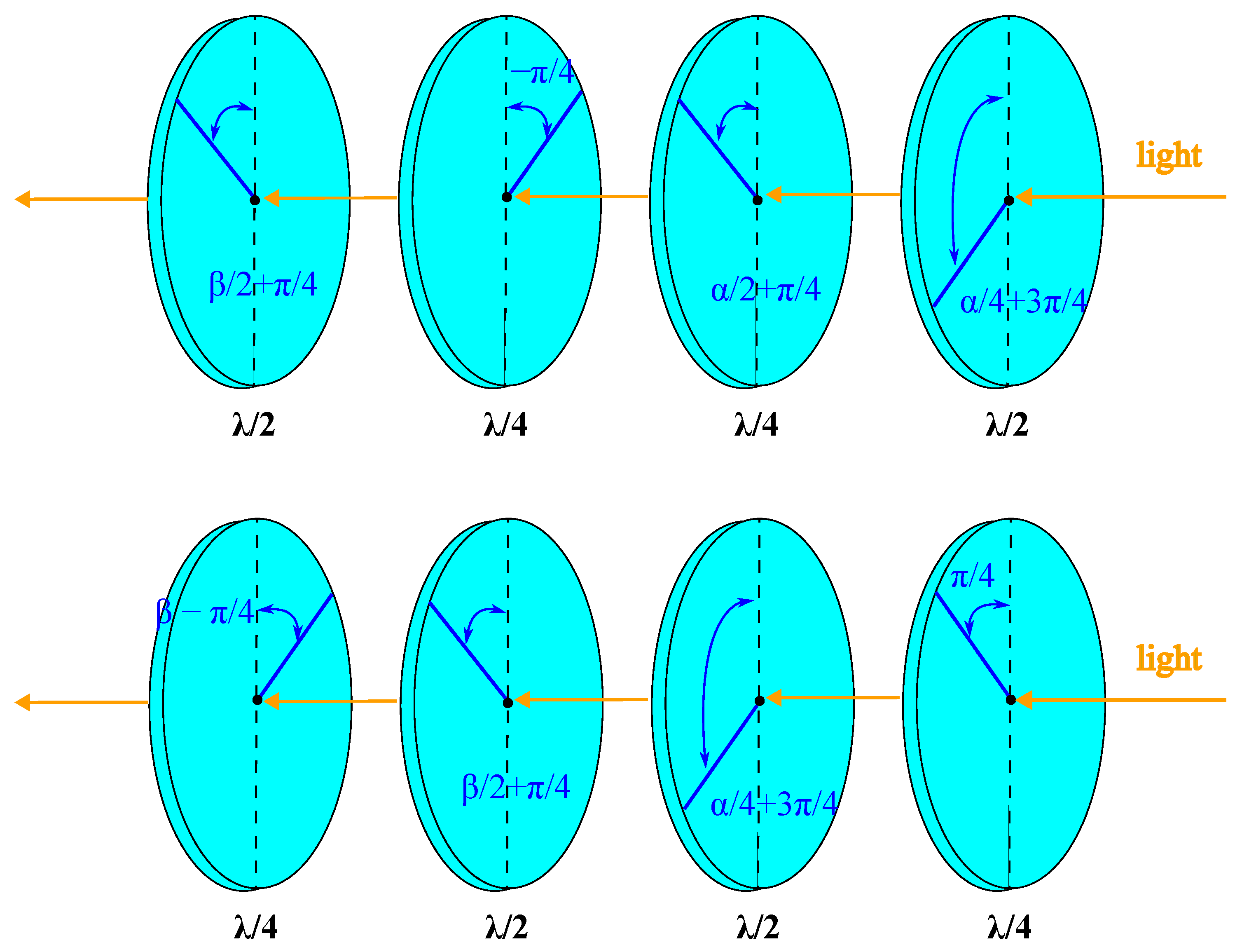
Figure 1 provides a schematic illustration of the polarization controllers corresponding to Equation (13b,c), implemented using two half-wave plates and two quarter-wave plates.

5. Misalignment Robustness Simulation of the Polarization Controller

To evaluate the practical robustness of our polarization controller design, we performed a numerical Monte Carlo simulation incorporating small random angular misalignments of the wave plates. These misalignments represent realistic mechanical uncertainties that occur during alignment or operation of the controller.

The specific controller configuration studied corresponds to Equation (13b), consisting of four wave plates in the following sequence:

$${\mathbf{J}}^R(\beta ,\alpha )={\mathbf{J}}_{{\theta }_4}\left(\pi \right){\mathbf{J}}_{{\theta }_3}(\pi /2){\mathbf{J}}_{{\theta }_2}(\pi /2){\mathbf{J}}_{{\theta }_1}\left(\pi \right),$$

(14)

where the orientation angles of the plates are as follows:

$$\begin{array}{cc}\hfill {\theta }_1& =\frac{3\pi }{4}+\frac{\alpha }{4},{\theta }_2=\frac{\alpha }{2}+\frac{\pi }{4},\hfill \end{array}$$

(15)

$$\begin{array}{cc}\hfill {\theta }_3& =-\frac{\pi }{4},{\theta }_4=\frac{\beta }{2}+\frac{\pi }{4},\hfill \end{array}$$

(16)

with $\alpha =\pi /4$ and $\beta =\pi /3$ for our simulation.

Each wave plate’s orientation angles (${\theta }_1$, ${\theta }_2$, ${\theta }_3$, and ${\theta }_4$) were perturbed by a small random offset sampled from a normal distribution with zero mean and a standard deviation of 1° (converted to radians for numerical calculations). The Jones matrix of each wave plate was computed, including the misalignment, and the total Jones matrix of the controller was obtained as the ordered matrix product of the four elements.

The input polarization state was taken as linear horizontal (${\mathbf{E}}_{\mathrm{in}}={[1,0]}^T$), and for each trial, the output Stokes vector was computed from the Jones vector. The deviation $\Delta S$ from the ideal Stokes vector (obtained without misalignment) was measured via the Euclidean norm.

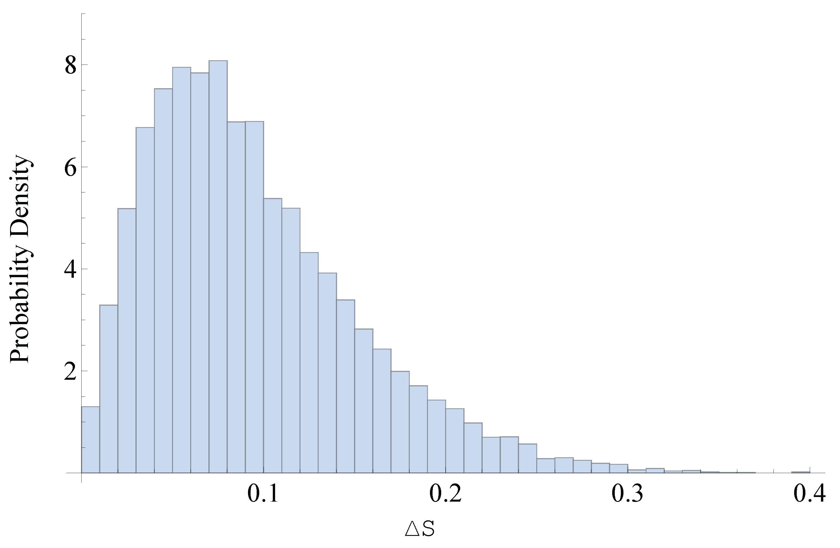
A total of 10,000 trials were performed to statistically sample the effect of misalignment. The resulting distribution of $\Delta S$ values is shown in Figure 2. The mean deviation was found to be as follows:

$$\begin{array}{cc}\hfill \langle \Delta S\rangle & =0.0941,\hfill \end{array}$$

(17)

$$\begin{array}{cc}\hfill \sigma (\Delta S)& =0.0574.\hfill \end{array}$$

(18)

This simulation demonstrates that the proposed four-plate controller is robust to small alignment errors. The average deviation remains below $0.1$ in Stokes space, which is acceptable for many experimental applications requiring polarization control with moderate precision.

6. Summary

In conclusion, we theoretically introduce several types of arbitrary polarization retarders constructed from sequences of half-wave and quarter-wave plates, each rotated at specific angles. By combining these arbitrary polarization retarders with arbitrary polarization rotators, we develop a versatile device capable of performing arbitrary-to-arbitrary polarization transformations. While some of the proposed devices are documented in the literature, others are novel and, to the best of our knowledge, have not been previously presented. The continuous adjustment of retardance and rotation in these devices is achieved by altering the relative orientation of the wave plates in the sequence.

While the present work focuses on fully polarized light and employs Jones calculus, the extension of our approach to partially polarized or depolarized light would require the use of the Mueller matrix formalism. Unlike the Jones method, which is limited to coherent and completely polarized beams, Mueller calculus allows for the treatment of incoherent, mixed, or depolarized states. Adapting the proposed wave plate configurations to operate within this broader framework could enable applications in imaging systems, scattering environments, and biological tissues where partial polarization is prevalent.

Our theoretical treatment assumes ideal wave plates with constant retardance over the operating wavelength range. However, in real-world applications, chromatic dispersion and the wavelength dependence of birefringence introduce deviations from ideal behavior. This leads to performance degradation when using standard wave plates, which are typically optimized for a single wavelength.

To construct an achromatic polarization retarder or controller, it is essential that each constituent wave plate (half-wave or quarter-wave) maintains its retardance across the desired spectral range. This requirement can be met by employing achromatic wave plates, which are specially engineered—often by stacking multiple birefringent plates of different materials and thicknesses—to compensate for dispersion effects [24,25,26]. Alternatively, Fresnel rhombs [16] can be used to realize highly achromatic phase retarders, as they introduce phase shifts through total internal reflection rather than birefringence, making them inherently less sensitive to wavelength variation.

When all individual components are achromatic, the resulting multi-plate system also behaves achromatically. Otherwise, the polarization transformation becomes wavelength-dependent, reducing the device’s effectiveness in broadband applications.