Simulation-Based Verification and Application Research of Spatial Spectrum Modulation Technology for Optical Imaging Systems

Abstract

Leveraging Fourier optics theory and Abbe’s imaging principle, this study establishes that optical imaging fundamentally involves selective spatial spectrum recombination at the Fourier plane. Three classical experiments quantitatively validate universal spectrum manipulation mechanisms: (1) The Abbe-Porter experiment confirmed spectral filtering, directly demonstrating image synthesis from transmitted spectral components. (2) Zernike phase-contrast microscopy quantified spectral phase modulation, overcoming the weak-phase-object detection limit by significantly enhancing contrast. (3) Optical joint transform correlation (JTC) demonstrated efficient spectral amplitude modulation for high-speed, high-accuracy image recognition. Collectively, these results form a comprehensive framework for active light field manipulation at the spectral plane, extending modulation capabilities to phase and amplitude dimensions. This work provides a foundational theoretical and technical framework for designing advanced optical systems, extending modulation capabilities to phase and amplitude dimensions.

1. Introduction

The advancement of optical imaging technology has consistently progressed alongside a deepening understanding of light field properties. The establishment of Fourier transform optics marked a fundamental shift in optical research from the spatial domain to the frequency domain. Its core innovation resides in introducing the concept of the spatial spectrum (defined as the two-dimensional Fourier transform F(u,v) of the object light field), thereby transforming intricate light propagation and imaging processes into linear operations within the spectral domain [1,2]. This not only elucidates the physical essence of optical imaging but also enables the development of optical information processing technologies based on active spatial spectrum modulation. Selective manipulation of the light field at the Fourier plane (e.g., filtering, phase modulation, or amplitude modulation [3,4,5]) enables controlled modulation of imaging outcomes. Additionally, Fourier transform techniques for incoherent optical processing and deep learning-assisted spectral optimization offer advanced methodologies for modern optical system design [6,7,8].

Abbe’s (Ernst Abbe) theory of secondary imaging represents the foundational work in this domain. This theory decomposes lens imaging into two physical processes: (1) Spectrum Generation: The object light field undergoes Fraunhofer diffraction at the Fourier plane through the lens, forming its spatial spectrum F(u,v); (2) Image Reconstruction: The spectral components propagate to the image plane and interfere coherently to form the image distribution. The classic Abbe–Porter experiment first demonstrated that placing spatial filters at the spectrum plane to actively suppress or enhance specific spectral components enables selective control of image structures. This experiment physically validated the core tenet that “the image is synthesized by the spectral components transmitted through the filter,” thereby establishing a rigorous foundation for spectrum manipulation techniques [9].

Within the Abbe theoretical framework, spectrum plane modulation techniques have progressively expanded into the following key application scenario: Breakthrough in Phase Modulation Dimension. In biological microscopic observation, transparent samples primarily exhibit weak phase modulation (ϕ(x,y) ≪ 1). Traditional bright-field microscopy fails due to its inability to respond to phase changes. Zernike phase-contrast microscopy overcame the bottleneck of “invisible” transparent samples by introducing a λ/4 plate (inducing a π/2 phase shift) at the center of the spectrum plane. This selectively modulates the phase of the zero-frequency component, breaking the phase orthogonality between direct and scattered light. It thus achieved the first linear conversion from phase distribution to image intensity change (ΔI ∝ ϕ) [10,11]. Extension to Amplitude Modulation and Joint Operations: To meet the demand for high-speed image recognition, the optical joint transform correlator (JTC), based on the Fourier transform cross-correlation theorem, directly performs amplitude modulation and filtering operations on the joint power spectrum at the spectrum plane. Subsequent inverse transformation yields a high signal-to-noise ratio (SNR) cross-correlation peak. This technique extends spectrum plane operations from single-object filtering to joint dual-image processing, significantly enhancing pattern recognition efficiency and parallelism [12,13,14].

Although Abbe imaging, Zernike phase-contrast, and JTC technologies target distinct application scenarios (microscopic imaging versus target recognition), their physical essence is unified through the active manipulation of the light field at the spectrum plane. Abbe’s principle reveals the theoretical origin and fundamental mechanism of spectral operations; Zernike phase-contrast achieves a key breakthrough in the phase modulation dimension; the joint transform correlator develops capabilities for amplitude modulation and joint spectral processing. Collectively, they constitute a complete technological chain for “light field manipulation in the spectral domain.” However, the intrinsic consistency and universality of their manipulation mechanisms have not yet been systematically verified within a unified theoretical and experimental framework.

To address this, this paper, based on Fourier optics theory combined with high-precision numerical simulation experiments, focuses on the core role of spatial spectrum modulation technology in imaging enhancement and information processing, as well as in conducting systematic research: 1.Analyze the Abbe–Porter experiment to quantitatively verify the selective extraction of image structures by directional filtering and the homogenization effect of zero-frequency filtering; 2. Construct a Zernike phase-contrast microscopy model to quantify the improvement in imaging contrast for weak-phase objects by spectral phase modulation and the resulting phase-intensity linear relationship; 3. Implement optical joint transform correlation recognition simulation to verify the optimization capability of joint power spectrum amplitude modulation on the positioning accuracy and SNR of the cross-correlation peak.

This study aims to establish a closed-loop verification system of “imaging (Abbe)–enhancement (Zernike)–recognition (JTC)” through these three typical experiments, elucidating the universal mechanism of spectrum plane manipulation. It seeks to provide solid theoretical and experimental foundations for the design optimization of complex optical systems, particularly in the fields of biological microscopic imaging and high-speed target recognition.

2. Theoretical Analysis

2.1. Abbe’s Secondary Imaging Principle

Taking a one-dimensional grating with binary transmittance values of 0 and 1 as an example, Fourier analysis is used to analyze Abbe’s secondary imaging principle and the role of spatial filtering [15].

For mathematical simplicity and neglecting the effect of the objective aperture size, the transmittance function of the one-dimensional grating at the object plane (x₀, y₀) can be expressed as follows [16]:

$$\begin{array}{l}\mathrm{f}(x_0)=\left[\mathrm{rect}\left({\displaystyle \frac{x_0}{a}}\right)\otimes {\displaystyle \frac{1}{d}}\mathrm{comb}\left({\displaystyle \frac{x_0}{d}}\right)\right]\mathrm{rect}\left({\displaystyle \frac{x_0}{L}}\right)\\ =\left[{\displaystyle \sum _{m=-\infty }^{\infty }\mathrm{rect}(\frac{x_0-md}{a})}\right]\mathrm{rect}({\displaystyle \frac{x_0}{L}})\end{array}$$

(1)

where a denotes the width of the transmitting slit, d represents the grating period, and L signifies the total width of the grating. The light field at the back focal plane of the objective (the spectrum plane) is given by

$$\begin{array}{l}\mathrm{F}\left(u\right)=\mathrm{F}\left\{\mathrm{f}(x_0)\right\}=[a\sin c(au)\mathrm{com}b(du)]\otimes L\sin c(Lu)\\ =aL[\sin c(au){\displaystyle \frac{1}{d}}{\displaystyle \sum _{m=-\infty }^{\infty }\delta (u-\frac{m}{d})}]\otimes \sin c(Lu)\\ ={\displaystyle \frac{aL}{d}}{\displaystyle \sum _{m=-\infty }^{\infty }\sin c(\frac{am}{d})}\sin c\left[L(u-{\displaystyle \frac{m}{d}})\right]\\ ={\displaystyle \frac{aL}{d}}\sin c(Lu)+{\displaystyle \frac{aL}{d}}\sin c({\displaystyle \frac{a}{d}})\sin c\left[L(u-{\displaystyle \frac{1}{d}})\right]+{\displaystyle \frac{aL}{d}}\sin c({\displaystyle \frac{a}{d}})\sin c\left[L(u+{\displaystyle \frac{1}{d}})\right]+\mathrm{\dots }\end{array}$$

(2)

where $u={\displaystyle \frac{x}{\lambda f}}$. λ is the wavelength of light, f is the focal length of the lens, and x is the spatial coordinate on the focal plane. The imaging at the image plane is analyzed below for different filters placed at the focal plane.

(1) Passing only the zero-order component:

The transmitted light field at the focal plane is

$$\mathrm{F}\left(u\right)\mathrm{H}\left(u\right)={\displaystyle \frac{aL}{d}}\sin c(Lu)$$

(3)

Therefore, the image at the image plane (with x_i as the spatial coordinate) is

$$\mathrm{f}\left(x_i\right)=\mathrm{rect}({\displaystyle \frac{x_i}{L}})$$

(4)

Evidently, the image plane exhibits uniform illumination without intensity variation, resulting in the complete loss of the periodic structure.

(2) Passing the zero-order and positive/negative first orders:

The transmitted light field at the focal plane is

$$\mathrm{F}\left(u\right)\mathrm{H}\left(u\right)={\displaystyle \frac{aL}{d}}\left\{\sin c(Lu)+\sin c({\displaystyle \frac{a}{d}})\sin c\left[L(u-{\displaystyle \frac{1}{d}})\right]+\sin c({\displaystyle \frac{a}{d}})\sin c\left[L(u+{\displaystyle \frac{1}{d}})\right]\right\}$$

(5)

The image at the image plane is

$$\mathrm{f}(x_i)=\mathrm{rect}\left({\displaystyle \frac{x_i}{L}}\right)\left[1+2\sin c\left({\displaystyle \frac{a}{d}}\right)\cos (2\pi {\displaystyle \frac{x_i}{d}})\right]$$

(6)

In this case, on the basis of the contribution from the zero-order, the image exhibits a periodic structure. However, due to the absence of higher-frequency information, the intensity distribution is flattened, the image contrast is reduced, and it becomes a cosine amplitude grating.

(3) Passing only the positive and negative second orders:

The transmitted light field at the focal plane is

$$\mathrm{F}\left(u\right)\mathrm{H}\left(u\right)={\displaystyle \frac{aL}{d}}\sin c({\displaystyle \frac{2a}{d}})\left\{\sin c\left[L(u-{\displaystyle \frac{2}{d}})\right]+\sin c\left[L(u+{\displaystyle \frac{2}{d}})\right]\right\}$$

(7)

The image at the image plane is

$$f(x_i)=rect\left({\displaystyle \frac{x_i}{L}}\right)\left[2\sin c\left({\displaystyle \frac{2a}{d}}\right)\cos (4\pi {\displaystyle \frac{x_i}{d}})\right]$$

(8)

Here, the image structure is that of a cosine amplitude grating, but its period is halved compared to the object. That is, the number of lines in the image plane is twice that of the object.

2.2. Zernike Phase-Contrast Microscopy

In biological microscopic observation, transparent specimens exhibit extremely weak light absorption. Their optical properties are primarily characterized by spatial phase modulation induced by variations in thickness/refractive index. Traditional bright-field microscopy, responding only to intensity information, cannot detect these phase changes, rendering the structure of such specimens invisible. Dutch physicist Frits Zernike, based on spatial spectrum modulation theory, proposed phase-contrast microscopy to solve this challenge. Its core principle lies in manipulating the zero-frequency phase at the spectrum plane to break the orthogonality between the undiffracted (direct) and diffracted (scattered) components of the object light. This achieves phase-to-intensity conversion, establishing for the first time a linear relationship between image intensity I and object phase ϕ, thereby enabling the topological structure of transparent specimens to be visualized as grayscale contrast.

Considering a transparent object with an amplitude transmittance function,

$$\mathrm{t}(x_0,y_0)=\exp [j\Delta \phi (x_0,y_0)]$$

(9)

This indicates the object induces negligible absorption but only a phase change. Assuming the phase change $\Delta \phi (x_0,y_0)$ caused by thickness variations is much smaller than 1, the amplitude transmittance can be approximated as

$$\mathrm{t}(x_0,y_0)=\exp [j\Delta \phi (x_0,y_0)]\approx 1+j\Delta \phi (x_0,y_0)$$

(10)

If uniform illumination with complex amplitude $\exp [j\Delta \phi (x_0,y_0)]$ passes through this object, the transmitted complex amplitude distribution is

$$\begin{array}{l}\mathrm{f}(x_0,y_0)=\mathrm{t}(x_0,y_0)\exp [j\Delta {\phi }_0(x_0,y_0)]\\ \approx \exp [j\Delta {\phi }_0(x_0,y_0)]+j\Delta \phi (x_0,y_0)\exp [j\Delta {\phi }_0(x_0,y_0)]\end{array}$$

(11)

Thus, the object light field can be effectively decomposed into two components: a strong undiffracted wave (zero-frequency component) and a weak diffracted wave (high-frequency, phase-modulated component) arising from phase variations. Consequently, the intensity obtained at the image plane in a conventional microscope is

$$\begin{array}{l}\mathrm{I}(x_i,y_i)\approx \left|\exp \left[j\Delta {\phi }_0(x_i,y_i)\right]\right|{\left[1+j\Delta \phi (x_i,y_i)\right]}^2\\ =1+\Delta \phi {(x_i,y_i)}^2\approx 1\end{array}$$

(12)

The object light field from a transparent sample comprises the undiffracted wave (zero-frequency component) and the diffracted wave (high-frequency, phase-modulated component). These two components possess a fixed π/2 phase difference. This phase orthogonality causes the interference effect at the image plane to vanish, preventing the phase information from being converted into observable intensity contrast.

Zernike proposed placing a phase plate at the center of the objective’s back focal plane (spectrum plane). Its key functions are as follows: (1) Selectively modulate the undiffracted wave phase: Introduce a π/2 or 3π/2 phase shift using a transparent dielectric film. (2) Reconstruct the interference condition: Adjust the phase difference between the undiffracted and diffracted waves to 0 or π, activating coherent interference. (3) Achieve phase-to-intensity transformation: Linearly map the phase distribution ϕ(x, y) to image intensity change ΔI ∝ ϕ.

For a π/2 phase shift applied to the undiffracted wave, the intensity at the image plane is (known as positive phase-contrast) as folows:

$$\begin{array}{l}\mathrm{I}(x_i,y_i)\approx {\left|\exp (j{\displaystyle \frac{\pi }{2}})+j\Delta \phi (x_i,y_i)\right|}^2={\left|j+j\Delta \phi (x_i,y_i)\right|}^2\\ \approx 1+2\Delta \phi (x_i,y_i)\end{array}$$

(13)

For a 3π/2 phase shift applied to the undiffracted wave, the intensity is (known as negative phase-contrast) as follows:

$$\begin{array}{l}\mathrm{I}(x_i,y_i)\approx {\left|\exp (j{\displaystyle \frac{3\pi }{2}})+j\Delta \phi (x_i,y_i)\right|}^2={\left|-j+j\Delta \phi (x_i,y_i)\right|}^2\\ \approx 1-2\Delta \phi (x_i,y_i)\end{array}$$

(14)

2.3. Optical Joint Transform Correlation Recognition

Mathematically, the similarity between two images f(x, y) and h(x, y) can be evaluated using the correlation operation. Their cross-correlation function is defined as

$${\mathrm{R}}_{fh}(x,y)={\displaystyle \int {\displaystyle {\int }_{-\infty }^{+\infty }\mathrm{f}\left(\alpha ,\beta \right)}}{\mathrm{h}}^{*}(\alpha -x,\beta -y)d\alpha d\beta$$

(15)

denoted as

$${\mathrm{R}}_{fh}(x,y)=\mathrm{f}\left(x,y\right)☆\mathrm{h}(x,y)$$

(16)

The correlation operation is related to convolution as

$${\mathrm{R}}_{fh}(x,y)=\mathrm{f}\left(x,y\right)☆{\mathrm{h}}^{*}(-x,-y)$$

(17)

Since spatial domain convolution is computationally intensive, the cross-correlation theorem of Fourier transforms is commonly used to shift the correlation operation into the frequency domain. Let the Fourier transforms of f(x, y) and h(x, y) be F(u, v) and H(u, v), respectively:

$$\mathrm{F}(u,v)=\mathrm{F}\left\{\mathrm{f}(x,y)\right\},\mathrm{H}(u,v)=\mathrm{F}\left\{\mathrm{h}(x,y)\right\}$$

(18)

Then:

$$\mathrm{F}\left\{\mathrm{f}(x,y)☆\mathrm{h}(x,y)\right\}={\mathrm{F}}^{*}(u,v)\mathrm{H}(u,v)$$

(19)

The result is then transformed back to the spatial domain. In the optical implementation, the target image f to be recognized and the reference image h are placed side-by-side on the object plane, with their centers located at (0, −b) and (0, +b), respectively. The object plane is illuminated by collimated monochromatic light of wavelength λ. The complex amplitude distribution of the object light field can be expressed as

$$\mathrm{u}(x_0,y_0)=\mathrm{f}(x_0,y_0-b)+\mathrm{h}(x_0,y_0+b)$$

(20)

At the back focal plane of the lens, the complex amplitude distribution is proportional to the Fourier spectrum of the incident light field:

$$\mathrm{U}(u,v)=\mathrm{F}(u,v)\exp (-j2\pi vb)+\mathrm{H}(u,v)\exp (j2\pi vb)$$

(21)

This complex amplitude distribution is converted by a square-law detector into the joint transform power spectrum (JTPS) distribution:

$$\mathrm{I}(u,v)={\left|\mathrm{U}(u,v)\right|}^2={\left|\mathrm{F}\right|}^2+{\left|\mathrm{H}\right|}^2+{\mathrm{F}}^{*}\mathrm{H}\exp (-j4\pi vb)+\mathrm{F}{\mathrm{H}}^{*}\exp (j4\pi vb)$$

(22)

In the above expression, the first term ${\left|F\right|}^2$ and the second term ${\left|H\right|}^2$ are the spectra of the autocorrelation functions $R_{ff}(x,y)$ and $R_{hh}(x,y)$ of image f and reference image h, respectively. The third term $F^{*}H\exp (-j4\pi vb)$ and fourth term $F{H}^{*}\exp (j4\pi vb)$ are the spectra of the cross-correlation functions $R_{fh}(x,y)$ and $R_{hf}(x,y)$ between f and h, but each is multiplied by a linear phase factor. This power spectrum undergoes a second diffraction (equivalent to an inverse Fourier transform, or more precisely, a Fourier transform) by a lens. The output at the correlation plane (image plane) is proportional to

$${\mathrm{U}}_i(x_i,y_i)=\mathrm{f}☆\mathrm{f}+\mathrm{h}☆\mathrm{h}+(\mathrm{f}☆\mathrm{h})\otimes \delta (y_i-2b)+(\mathrm{h}☆\mathrm{f})\otimes \delta (y_i+2b)$$

(23)

Clearly, correlation peaks corresponding to f and h appear at positions (0, 2b) and (0, −2b) in the output plane, respectively. The higher the intensity (brightness) of a peak, the greater the similarity between the images f and h. Conversely, lower similarity results in dimmer, diffused spots [17].

3. Simulation Verification

3.1. Numerical Simulation Flow of the Abbe–Porter Experiment

(1) Initial Optical System Parameter Settings (See

Table 1. Experimental optical parameters.

Parameter	Symbol	Value	Physical Meaning
Wavelength	λ	632.8 nm	He-Ne laser wavelength
Lens focal length	f	4 mm	Fourier transform lens
Object plane size	L0	1 mm	Grating spatial extent
Grating period	d	30 pixels	Corresponding physical size: 58.6 μm
Filter diameter	D1	50 μm	Low-pass filter size
Filter width	D2	50 μm	Directional filter size
Object distance	d0	4.1 mm	Distance from object plane to lens

)

(2) Light Field Propagation Calculation

• From object plane to lens front surface: Calculate the diffracted light field using the Single Fast Fourier transform (S-FFT) algorithm, recording the complex amplitude distribution at the lens incident surface.
• Lens phase modulation: Apply the lens transmittance function to obtain the complex amplitude distribution at the lens rear surface.

(3) Spectrum Plane Operation

• Back focal plane calculation: Apply the S-FFT algorithm to obtain the light field distribution at the spectrum plane (Fourier plane).
• Spatial filtering implementation: Generate three types of filters (H1: circular low-pass, H2: horizontal band-pass, H3: vertical band-pass). Compute the filtered spectrum (H1: passes near-zero frequency, H2: passes y-direction spectra, H3: passes x-direction spectra).

(4) Image Plane Reconstruction and Analysis

• Image field calculation: Perform an inverse S-FFT transform on the filtered spectrum to obtain the image plane intensity I(x, y) for four cases (including the unfiltered baseline).
• Result characterization: Visualize filtered and unfiltered reconstructed images; plot intensity profiles along characteristic directions; quantitatively compare the impact of filtering on imaging.

Figure 1 presents the simulation results of the Abbe–Porter experiment.

(1) Figure 1a Object distribution (2D grating): Displays a two-dimensional orthogonal grating structure with binary transmittance (0 or 1). Bright regions (U₀ = 1) and dark regions (U₀ = 0) alternate.

(2) Figure 1b Intensity distribution at lens front surface: The diffraction pattern formed after the object light propagates d₀ = 4.1 mm to the lens front surface. The central region exhibits the highest intensity with symmetric diffraction fringes, while significant intensity attenuation occurs at the edges.

(3) Figure 1c Intensity distribution at back focal plane (spectrum plane): The spatial spectrum at the lens back focal plane (f = 4 mm). The central zero-frequency component is the brightest, forming a symmetric lattice pattern (corresponding to the grating spatial frequencies), with the intensity of outer high-frequency components decreasing progressively.

(4) Filter Design (Figure 1d–f): H1 (Low-pass filter, Figure 1d) blocks high-frequency components, resulting in image blurring and reduced contrast. This validates that high-frequency information determines image detail. H2 (Horizontal band-pass, Figure 1e) and H3 (Vertical band-pass, Figure 1f) act as directional filters, selectively transmitting spectral components in a single direction (y-direction for H2, x-direction for H3). This causes the image to retain only vertical or horizontal stripes, respectively, confirming that the image structure is synthesized by the spectral components passing through the filter. Contrast comparison: The unfiltered case has the highest contrast. H1 filtering yields the lowest contrast due to high-frequency loss. H2/H3 filtering maintains high contrast due to directional selectivity.

(5) Reconstructed Image Comparison:

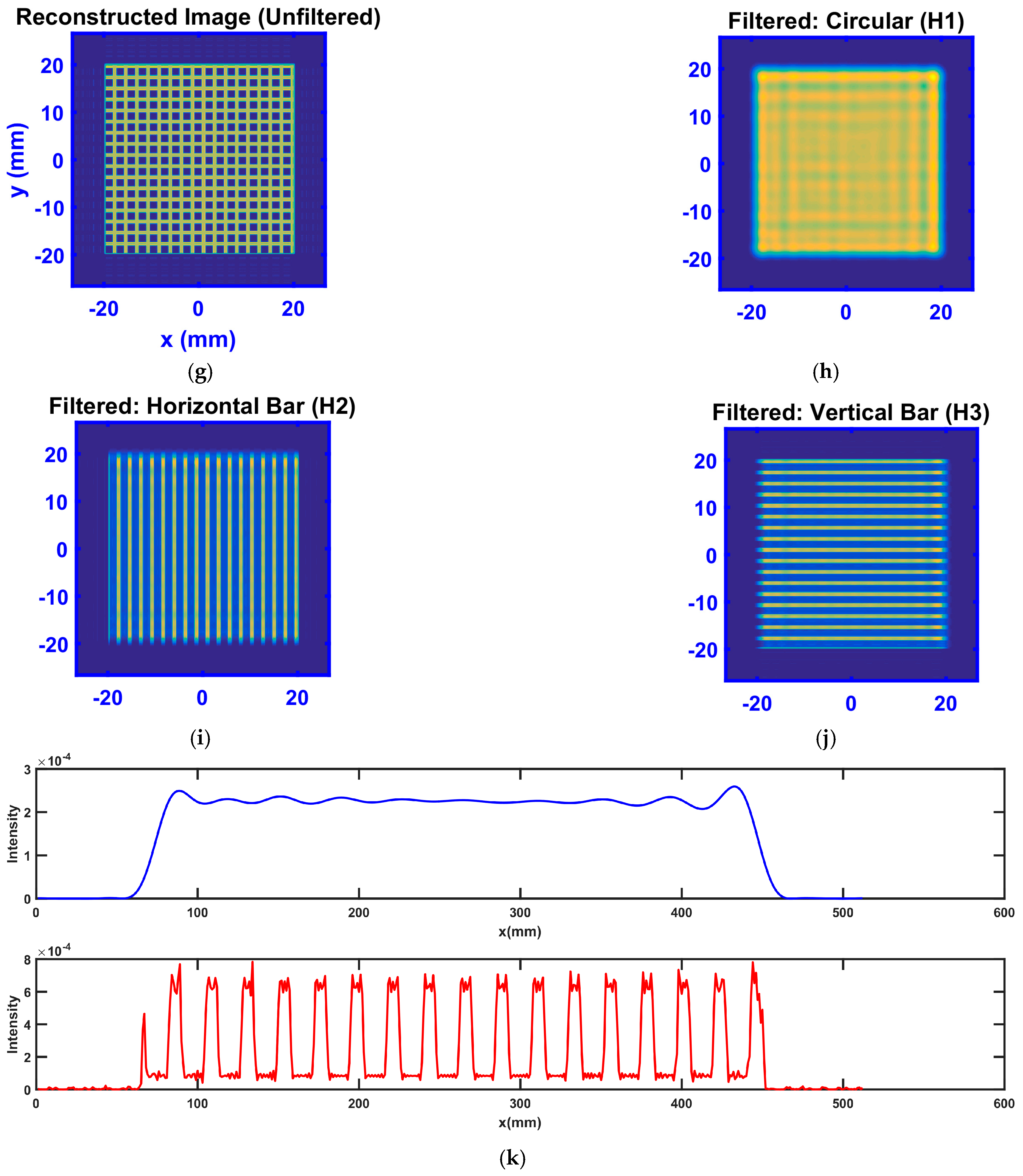
• Unfiltered (Figure 1g): Faithfully reproduces the full 2D grating structure. Slight diffraction effects are present at the edges. The intensity profile shows a rectangular wave distribution.
• H1-filtered (Figure 1h, Circular low-pass): Uniform intensity field with no periodic structure. Only the zero-frequency component passes, losing all spatial-frequency information. The intensity profile is approximately a horizontal line.
• H2-filtered (Figure 1i, Horizontal band-pass): Retains only vertical stripes (1D grating). Transmission of y-direction spectral components. Ripples appear at the top due to the inability of the physical filter to perfectly isolate high frequencies and boundary effects from discrete sampling in the simulation.
• H3-filtered (Figure 1j, Vertical band-pass): Retains only horizontal stripes (1D grating). Transmission of x-direction spectral components is clear. Ripples exist on the sides for the same reasons as in (3).

Summary: H1 filtering homogenizes the image plane (zero-frequency dominance), while H2/H3 achieve directional selective imaging.

• Profile Lines (Figure 1k): The profile for H1 filtering is approximately a horizontal line. The profile for H2 filtering shows periodic distribution, verifying directional selectivity.

The experiment employed a 2D grating object within a single-lens imaging system. By introducing different spatial filters (H1: circular low-pass, H2: horizontal band-pass, H3: vertical band-pass) at the back focal plane (spectrum plane), the characteristics of the image plane intensity distribution were analyzed under four conditions (unfiltered, H1, H2, H3). Analysis of structure, contrast, and output image information (

Table 2. Key metrics from Abbe–Porter experiment simulation.

Filter	Type	Structure Transmitted	Contrast	Output Image
None	None	Unobstructed	High	Clear 2D grid
H1	Circular LPF	D1 = 51 μm	Zero-frequency only	Blurred spot (HF loss)
H2	Horizontal BPF	D2 = 51 μm	y-direction only	Vertical bright lines
H3	Vertical BPF	D2 = 51 μm	x-direction only	Horizontal bright lines

) validates that the image structure is determined by the selection of spectral components. Directional filters successfully extract structural information along specific orientations of the object.

3.2. Numerical Simulation Procedure for Zernike Phase-Contrast Microscopy

(1) Initial Parameter Setup: Load the phase object image; generate the pure-phase object wavefield; set optical system parameters identical to those in Table 1.

(2) Diffraction Propagation from Object Plane to Lens Front Surface: Calculate the diffracted object wavefield using the S-FFT algorithm to obtain the complex amplitude distribution U1 on the lens front surface.

(3) Lens Phase Modulation: Apply the objective lens transmission function to modulate the wavefield, yielding the modulated wavefield at the lens rear surface.

(4) Spectrum Plane Field Calculation and Filtering: Obtain the spectrum Uf at the back focal plane using the S-FFT algorithm; construct positive/negative phase-contrast filters; generate the filtered wavefield.

(5) Image Plane Reconstruction and Comparative Analysis: Perform S-FFT inverse transforms on the three wavefields (unfiltered, positive contrast, negative contrast) to compute the image plane intensity distributions: I_unfiltered, I_{positive contrast}, I_{negative contrast}. .

(6) Quantitative Result Characterization: Visualize the three imaging results; plot intensity profiles along characteristic directions; calculate key metrics: contrast and phase response linearity.

Simulation results of Zernike phase-contrast microscopy are shown in Figure 2.

(1) Original phase object distribution (Figure 2a): A snowflake-shaped pure-phase object (phase range: 0–2π).

(2) Intensity distribution on the lens front surface (Figure 2b): The phase object propagated by diffraction to the objective front surface exhibits weak modulation fringes. This distribution reflects the object’s diffraction characteristics without direct phase-contrast information.

(3) Intensity distribution at the focal plane (spectrum plane) (Figure 2c): The Fourier spectrum displayed on a logarithmic scale. A central bright spot (zero-frequency component, direct transmitted light) is surrounded by a weak outer ring (high-frequency components, scattered light), indicating spatial separation of direct and scattered light.

(4) Ideal low-pass filter (Figure 2d): A circular filter with diameter D1 = 42 pixels, suppressing high-frequency noise but sacrificing resolution.

(5) Reconstructed image without phase-contrast (Figure 2e): A uniformly dark image with indiscernible phase structure.

(6) Reconstructed image with positive phase-contrast (Figure 2f): Imaging result with a + π/2 phase shift applied to the zero-frequency component. Bright background with dark structures (negative contrast) clearly outlines the snowflake contour.

(7) Reconstructed image with negative phase-contrast (Figure 2g): Imaging result with a + 3π/2 phase shift applied to the zero-frequency component. Dark background with bright structures (positive contrast) enhances central details.

(8) Comparison of theoretical and experimental results (Figure 2h): Top panel (Experimental): Black line; Theoretical curve: Red line; exhibiting perfect antisymmetry. Bottom panel (Experimental): Black line: Intensity profile of negative contrast; Red line: Intensity profile of positive contrast; showing excellent agreement with theoretical predictions.

The observed asymmetry in the experimental profile (Figure 2h, lower panel) near horizontal coordinates 120/320 is attributed to the following factors: 1. High-Frequency Information Loss. The Zernike phase-contrast microscopy experiment employed a circular low-pass filter designed to suppress high-frequency noise. However, this inherently attenuates high-frequency spatial details. The suppression of high-frequency components at object edges leads to distorted reconstruction of the fine contours of the phase object (snowflake structure), manifesting as the observed profile asymmetry. 2. Numerical Discretization Effects. The simulation program utilized discrete sampling (object plane resolution: 512 × 512 pixels) and the Single Fast Fourier Transform (S-FFT) algorithm for diffraction field calculation. Potential artifacts introduced by the discrete Fourier transform, such as spectral leakage and boundary truncation effects, may contribute to reconstruction errors and exacerbate the asymmetry.

Kurata et al. [18] utilized an annular aperture for background light suppression and phase-contrast enhancement. This approach offers the potential advantage of selectively filtering out the direct (undiffracted, zero-frequency) light while preserving medium-to-high-frequency scattered light components, thereby avoiding the detail loss inherent in low-pass filtering. By suppressing the background intensity, it directly enhances the contrast at the edges and within the interior of phase objects.

In contrast, this study employed a low-pass filter (rather than an annular aperture) based on the following rationale: 1. Focus on Core Theory Validation. The primary objective was to streamline the validation of the core theoretical principle of Zernike phase-contrast microscopy—namely, the phase-to-intensity conversion efficacy achieved through zero-frequency phase modulation (±π/2). The low-pass filter simplifies the model by focusing analysis on this key mechanism. 2. Noise Suppression Requirement. The low-pass filter provides effective suppression of high-frequency noise, significantly improving the signal-to-noise ratio (SNR), albeit at the cost of reduced spatial resolution.

The system study reveals the enhancement mechanism of phase visualization through phase-contrast filtering.

Table 3. Key metrics from Zernike phase-contrast microscopy simulation.

Imaging Mode	Phase Conversion	Intensity Distribution	Contrast	SNR	Resolution
No Phase-Contrast	None	Uniform gray background	0	Low	High-frequency information filtered, significant detail loss
Positive Contrast	+90°	Bright in high-phase regions	High (bright field)	Zero-order filtering reduces noise	Detail recognition improved
Negative Contrast	−90°	Dark in high-phase regions	Comparable to positive contrast but opposite polarity; high (dark field)	Zero-order light reduces noise	Structures clearly resolved

indicates the following: 1. Positive/Negative contrast converts phase information into intensity variations, enhancing contrast and SNR, thus resolving the invisibility of phase objects without contrast. 2. Positive contrast highlights phase-retarded regions (bright features), while negative contrast highlights phase-advanced regions (dark features), with comparable contrast and SNR between them.

3.3. Simulation Procedure for Optical Joint Transform Correlation Recognition

• System Initialization: Load the target image and reference image; set optical system parameters identical to those in Table 1.
• Diffraction Calculation from Object Plane to Lens Front Surface: Simulate object wave propagation using the S-FFT algorithm to calculate the wavefield distribution on the lens front surface.
• Lens Phase Modulation: Apply the lens transmission function to output the modulated wavefield at the lens rear surface.
• Acquisition of Spectrum at Lens Back Focal Plane: Compute the Fourier spectrum using the S-FFT algorithm; record the joint power spectrum distribution.
• Reconstruction from Spectrum Plane to Image Plane: Perform an inverse S-FFT on the power spectrum to calculate the intensity distribution at the output plane.
• Recognition Result Analysis: Visualize correlation peak distribution; plot intensity profiles; determine similarity based on peak location and intensity.

As shown in Figure 3, the simulation results of optical joint transform correlation recognition are presented:

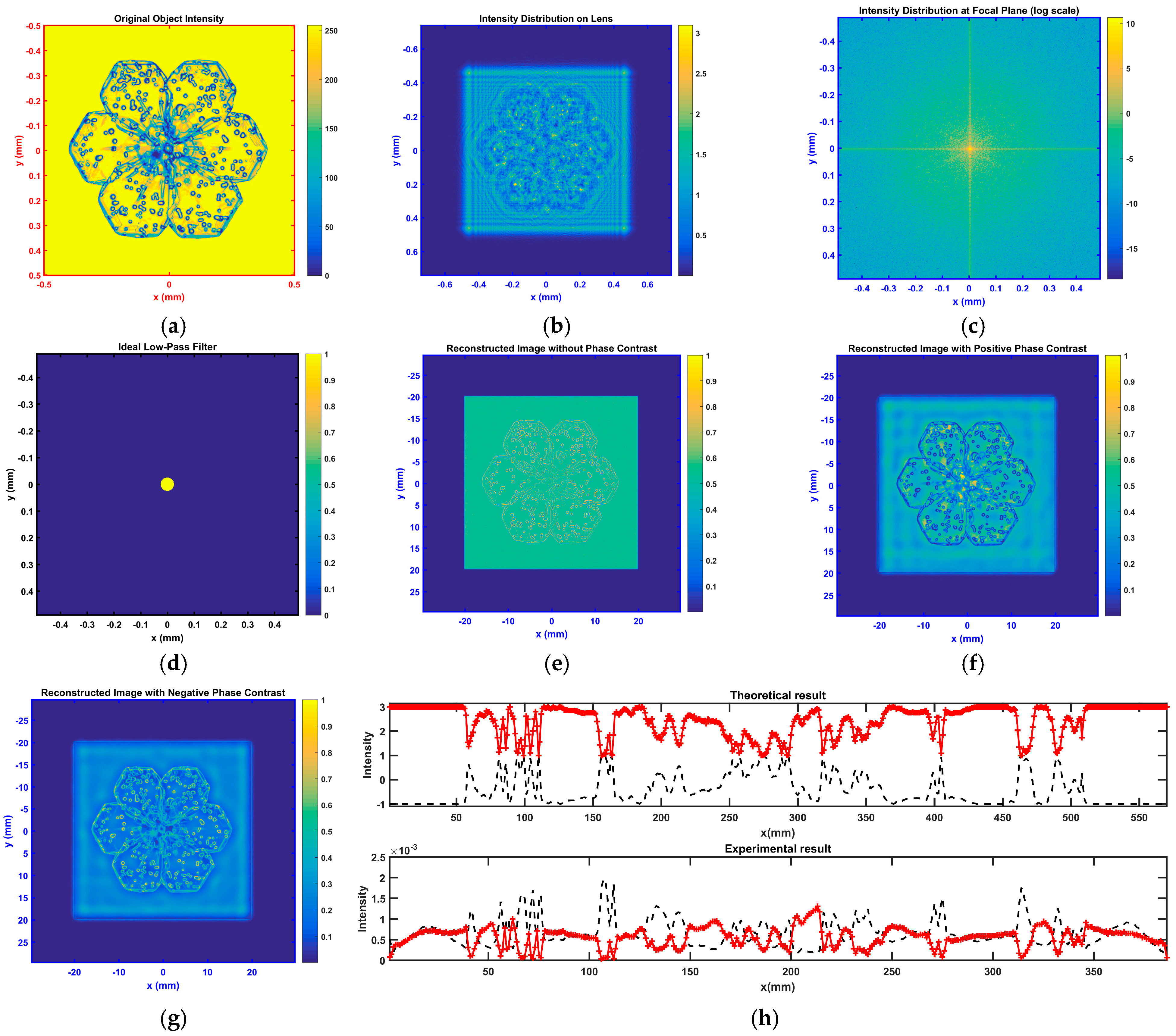
• Input image (object plane distribution) (Figure 3a): Juxtaposition of the target image (“ABCDEFGH”) and the reference image (“A”). The reference image “A” is positioned at the bottom, with the target string above. Binarization processing provides satisfactory contrast and sharp edges.
• Intensity distribution on the front surface of the lens (Figure 3b): Central bright spot: Zero-frequency component, corresponding to the average intensity of the target; Diffraction rings: Diffraction manifestation of high-frequency target information.
• Intensity distribution at the focal plane (spectrum plane) (Figure 3c): Central bright spot: Zero-frequency DC component; Symmetrical side lobes: Interference fringes from target/reference images; Modulated fringes: Phase modulation caused by spatial position differences among the targets.
• Reconstructed image intensity distribution (Figure 3d): Central bright spot: Zero-order diffraction; Symmetrical side peaks: Cross-correlation peaks.
• Three-dimensional intensity distribution (Figure 3e): 3D visualization of correlation peaks. The steep-sloped cross-correlation peak indicates high matching fidelity.
• Intensity profile analysis (Figure 3f): Cross-correlation peak height is significantly higher than the background (high SNR), with narrow peak width (good resolution).

This study achieves peak position alignment through symmetry compensation (via flip operations) and a predetermined spacing design. Similarity is indirectly calculated through the morphological analysis (intensity, width, signal-to-noise ratio) of cross-correlation peaks.

Table 4. Key metrics from optical joint transform correlation recognition simulation.

Metric	Physical Significance	Value/Feature	Impact on System Performance
Cross-correlation peak	Spatial matching degree between target and reference	Symmetrically distributed around zero-order peak	High matching fidelity
Peak intensity	Similarity between reference and target	Nearly 1 after normalization	High matching fidelity, strong noise immunity
Peak width	Sharpness of correlation peak	Extremely narrow (visible in profile)	Sub-pixel localization accuracy
SNR	Ratio of peak intensity to background noise	High SNR achieved via frequency domain filtering and diffraction optimization	Significant background noise suppression
Contrast	Intensity difference between peak and background	High contrast output from binarization and optical Fourier transform	Excellent distinction between target and background

indicates the following: (1) High SNR and contrast confirm effective background noise suppression; (2) Extremely narrow peak width provides sub-pixel localization accuracy; (3) Normalized peak intensity approaching 1 reflects high-target matching fidelity.

4. Conclusions

Grounded in Fourier optics theory, this study systematically establishes a comprehensive theoretical framework through three classical experiments: Abbe imaging, Zernike phase-contrast microscopy, and optical joint transform correlation recognition. These collectively elucidate the value of spatial-frequency domain transformation in core processes including imaging, enhancement, and recognition. Key conclusions are as follows: 1. Abbe–Porter experiment successfully demonstrated the modulation effect of spectral filtering on the image structure. Experiments demonstrate that directional selective filtering (e.g., horizontal/vertical band-pass) can precisely extract specific directional features of an object’s structure, while zero-frequency point filtering results in uniform intensity at the image plane. This directly validates the core tenet of Abbe’s imaging principle—the image is synthesized by the frequency components passing through the spectrum filter. 2 Zernike phase-contrast microscopy experiment quantitatively validated the efficacy of spectral phase modulation. By applying specific phase modulation (±π/2) at the zero-frequency point in the spectrum plane, this technique elevates the imaging contrast of pure-phase objects from nearly zero (without phase-contrast) to an observable level. It establishes a linear relationship between the phase distribution ϕ and the image intensity modulation ΔI (ϕ ∝ ΔI), effectively overcoming the challenge of insufficient contrast in transparent specimen imaging. 3. Optical joint transform correlation recognition experiment confirmed the high efficiency of joint spectrum amplitude modulation. The output cross-correlation peaks exhibit sub-pixel localization accuracy and high signal-to-noise ratio (SNR), indicating that modulation of the joint power spectrum in the frequency plane enables high-speed, high-precision image recognition. The Abbe imaging principle lays the theoretical foundation for spatial spectrum manipulation, clarifying how image structures are synthesized from selected spectral components. Zernike phase-contrast principle: Expanded the dimension of spectral modulation, achieving effective conversion of phase information (ϕ) into intensity information (ΔI) through phase manipulation at the zero-frequency point. Joint transform correlator principle: Extended amplitude modulation and joint filtering capabilities, optimizing cross-correlation performance via power spectrum modulation.

In the field of microscopic imaging, Zernike phase-contrast microscopy overcomes the observability barrier for transparent specimens through spectral phase modulation. In pattern recognition, the joint transform correlator utilizes spectral amplitude modulation to achieve parallel high-speed processing. Both share the common physical foundation of Abbe’s secondary imaging theory, demonstrating the universality and power of the spatial spectrum modulation framework.

Through quantitative simulations—investigating directional filter selectivity, phase-to-intensity conversion linearity, and cross-correlation peak localization accuracy—this study establishes a theoretical foundation for designing complex optical systems (e.g., super-resolution imaging systems, real-time target recognition systems).

References

1. Zhang, H.X.; Zhang, X.; Qiu, H.R.; Zhou, H. Automatic wavefront reconstruction on single interferogram with spatial carrier frequency using Fourier transform. Optoelectron. Lett. 2020, 16, 75–80. [Google Scholar] [CrossRef]
2. Nakayama, S.; Toba, H.; Fujiwara, N.; Gemma, T.; Takeda, M. Enhanced Fourier-transform method for high-density fringe analysis by iterative spectrum narrowing. Appl. Opt. 2020, 59, 9159–9164. [Google Scholar] [CrossRef]
3. Liu, Y.; Sun, Q.; Chen, H.; Jiang, Z. Fractional Fourier-transform filtering and reconstruction in off-axis digital holographic imaging. Opt. Express 2023, 31, 10709–10719. [Google Scholar] [CrossRef]
4. Javed, A.; Lüttig, J.; Sanders, S.E.; Sessa, F.; Gardiner, A.T.; Joffre, M.; Ogilvie, J.P. Broadband rapid-scanning phase-modulated Fourier transform electronic spectroscopy. Opt. Express 2024, 32, 28035–28047. [Google Scholar] [CrossRef]
5. You, J.; Wu, X.; He, H.; Xiao, Q.; Zeng, Y.; Chen, Y.; Dong, Z. Experimental comparison of discrete Fourier transform-spread high-order quadrature amplitude modulation discrete multitone systems for optical interconnection. Opt. Eng. 2019, 58, 076101. [Google Scholar] [CrossRef]
6. Chung, Y.; Hugonnet, H.; Hong, S.M.; Park, Y. Fourier space aberration correction for high resolution refractive index imaging using incoherent light. Opt. Express 2024, 32, 18790–18799. [Google Scholar] [CrossRef]
7. Fan, Y.; Sun, J.; Shu, Y.; Zhang, Z.; Zheng, G.; Chen, W.; Zhang, J.; Gui, K.; Wang, K.; Chen, Q.; et al. Efficient Synthetic Aperture for Phaseless Fourier Ptychographic Microscopy with Hybrid Coherent and Incoherent Illumination. Laser Photonics Rev. 2023, 17, 2200201. [Google Scholar] [CrossRef]
8. Zeng, H.; Yu, Y.; Liu, G.; Wu, Y. A Robust Method Based on Deep Learning for Compressive Spectrum Sensing. Sensors 2025, 25, 2187. [Google Scholar] [CrossRef]
9. Breuer, G. A Formal Representation of Abbe’s Theory of Microscopic Image Formation. Opt. Eng. 1984, 31, 661–670. [Google Scholar] [CrossRef]
10. Zernike, F. Phase contrast, a new method for the microscopic observation of transparent objects. Physica 1942, 9, 686–698. [Google Scholar] [CrossRef]
11. Nave, C. Phase contrast, A comparison of absorption and phase contrast for X-ray imaging of biological cells. J. Synchrotron Radiat. 2018, 25, 1490–1504. [Google Scholar] [CrossRef]
12. Lin, C.; Han, Y.; Lou, S.; Liu, P.; Zhang, W.; Yang, Z. Distortion-Invariant Target Recognition Based on Multichannel Joint Transform Correlator. Chin. J. Lasers 2022, 49, 686–698. [Google Scholar]
13. Wang, H.; Sun, H.; Zhao, X.; Wang, L.; Zhang, Q. The Design of the Real-Time Joint Transform Image Correlation Recognition System. Appl. Phys. 2019, 9, 348–355. [Google Scholar] [CrossRef]
14. Qian, Y.; Hong, X.; Miao, H. Improved target detection and recognition in complicated background with joint transform correlator. Optik 2013, 124, 6282–6285. [Google Scholar] [CrossRef]
15. Fitio, V.; Bendziak, A.; Yezhov, P.; Hryn, V.; Sakhno, O.; Smirnova, T. Diffraction of a finite-cross-section light beam by the grating: Theoretical analysis and experimental verification. Optik 2022, 252, 168550. [Google Scholar] [CrossRef]
16. Jing, X.; Jin, Y. Transmittance analysis of diffraction phase grating. Appl. Optics 2011, 50, C11–C18. [Google Scholar] [CrossRef]
17. Mohapatra, J.B.; Monikantan, J.; Nishchal, N.K. Object recognition under bad weather conditions with wavelet-modified logarithmic fringe-adjusted joint transform correlator. J. Opt. 2024. [Google Scholar] [CrossRef]
18. Kurata, R.; Toda, K.; Ishigane, G.; Naruse, M.; Horisaki, R.; Ideguchi, T. Single-image phase retrieval for off-the-shelf Zernike phase-contrast microscopes. Opt. Express 2024, 32, 2202–2211. [Google Scholar] [CrossRef]
Figure 1. Simulation results of the Abbe–Porter experiment (using three different filters). (a) Object (2D grating); (b) Intensity distribution on the lens front surface; (c) Intensity distribution at the back focal plane; (d) Filter 1 (‘H1’); (e) Filter 2 (‘H2’); (f) Filter 3 (‘H3’); (g) Reconstructed image without filter; (h) Reconstructed image with ‘H1’ filter; (i) Reconstructed image with ‘H2’ filter; (j) Reconstructed image with ‘H3’ filter; (k) Profile lines (lateral) of images filtered by ‘H1’ and ‘H2’.
Photonics 12 00755 g001aPhotonics 12 00755 g001b
Figure 2. Simulation results of Zernike phase-contrast microscopy. (a) Object (pure-phase object); (b) Intensity distribution on the lens front surface; (c) Intensity distribution at the back focal plane; (d) Ideal low-pass filter; (e) Reconstructed image without phase-contrast; (f) Reconstructed image with positive phase-contrast; (g) Reconstructed image with negative phase-contrast; (h) Theoretical experimental comparison.
Photonics 12 00755 g002
Figure 3. The simulation results of optical joint transform correlation recognition. (a) Object (Target to be recognized); (b) Intensity distribution on the lens front surface; (c) Intensity distribution at the back focal plane; (d) Reconstructed image intensity distribution; (e) 3D intensity display; (f) Intensity profile.
Photonics 12 00755 g003