A Dual-Wavelength Lidar Boundary Layer Height Detection Fusion Method and Case Analysis


Abstract
1. Introduction
2. Data and Methods
2.1. Observation Site
2.2. Instruments
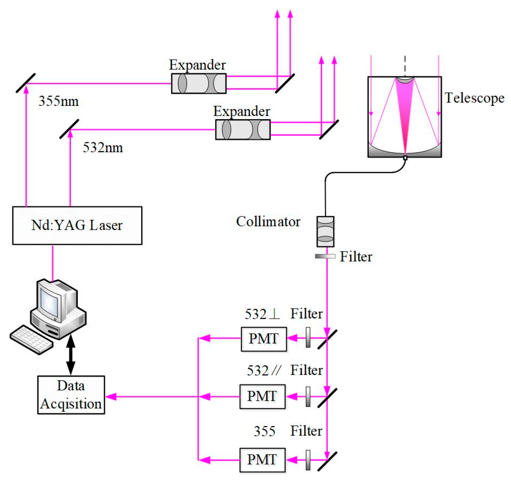
2.2.1. Lidar
2.2.2. Radiosonde
2.2.3. ERA5
2.3. Different ABLH Algorithms
2.3.1. Traditional Lidar ABL Algorithm
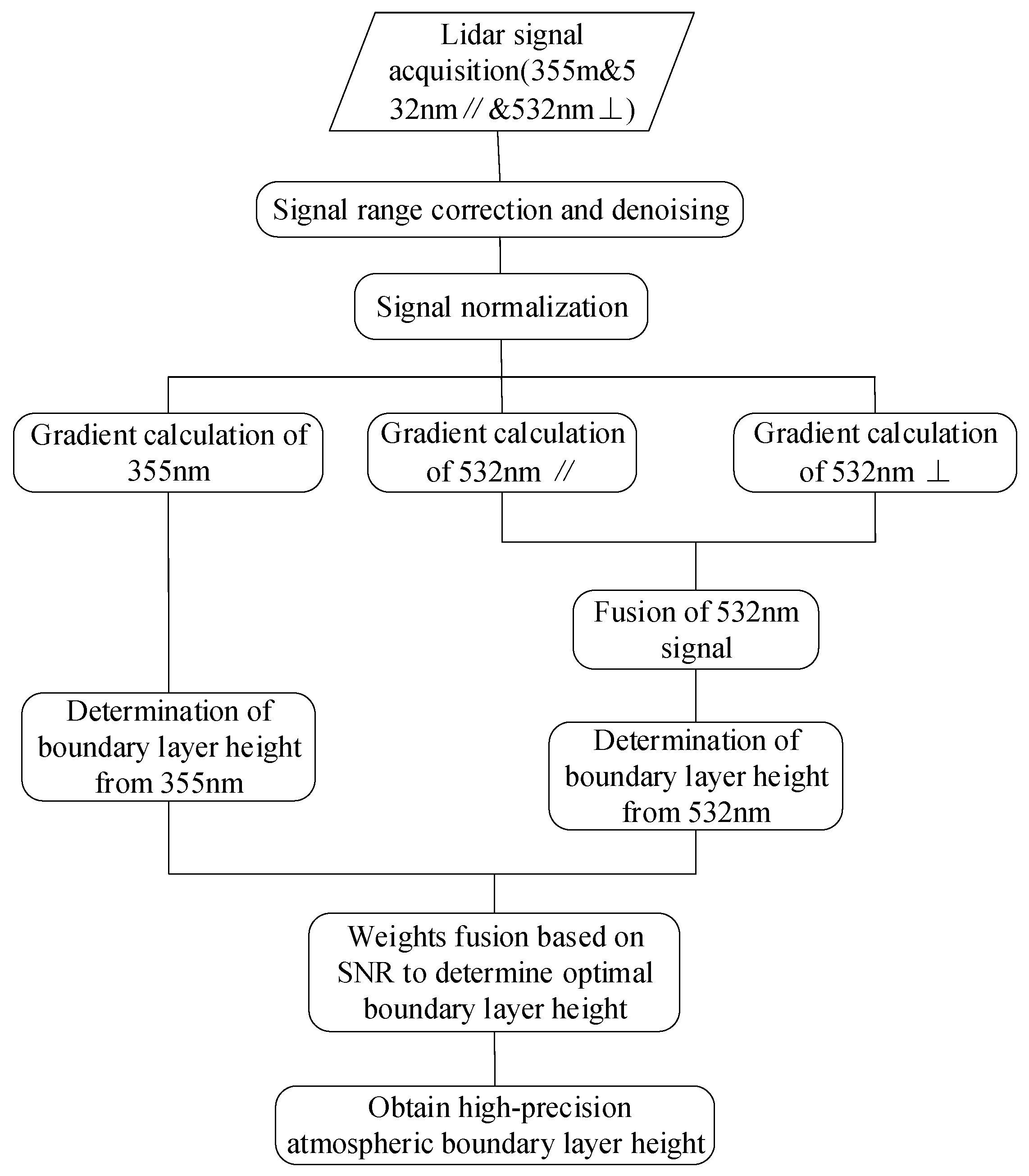
2.3.2. New Fusion Algorithm
2.3.3. Richardson Number Method
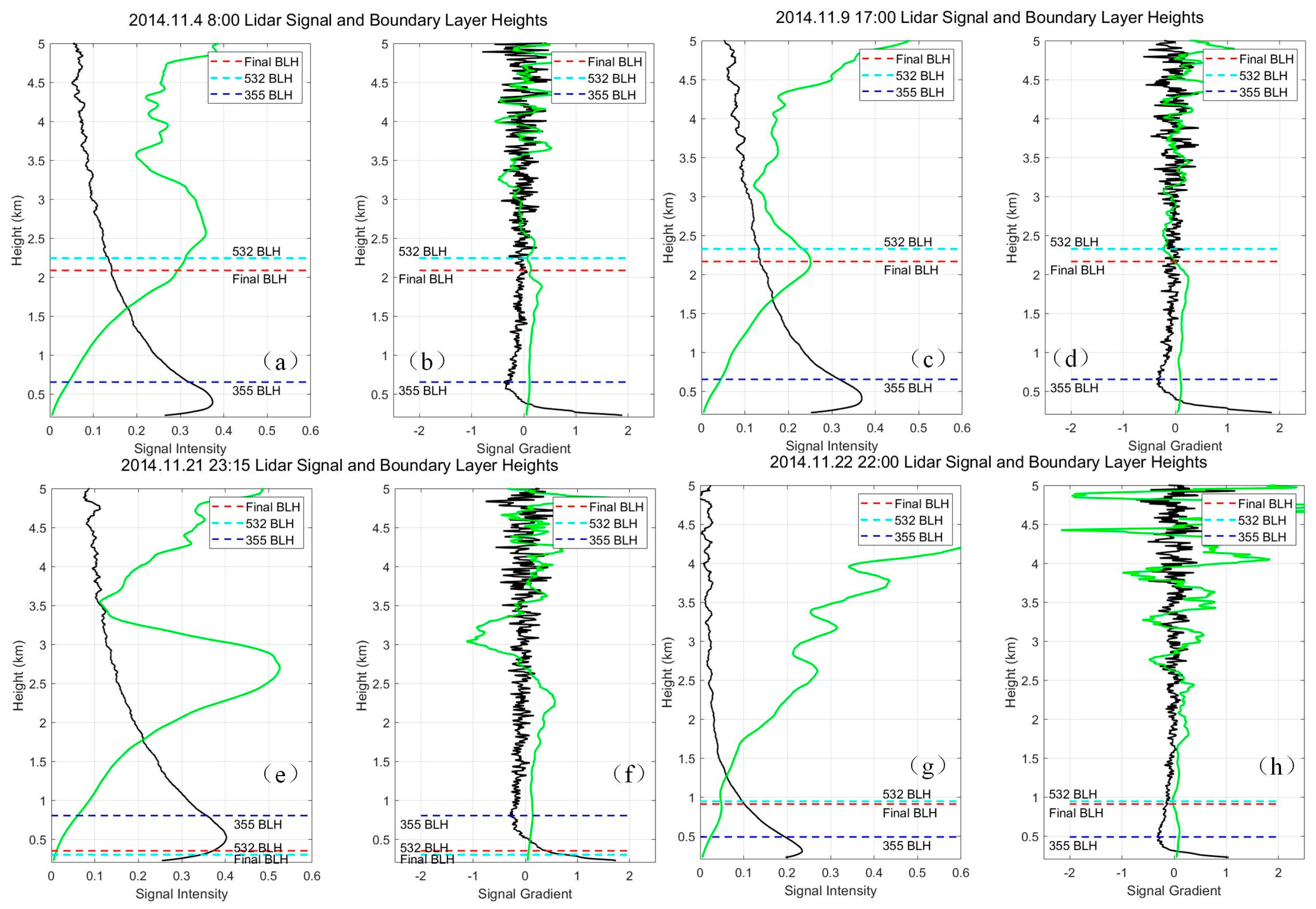
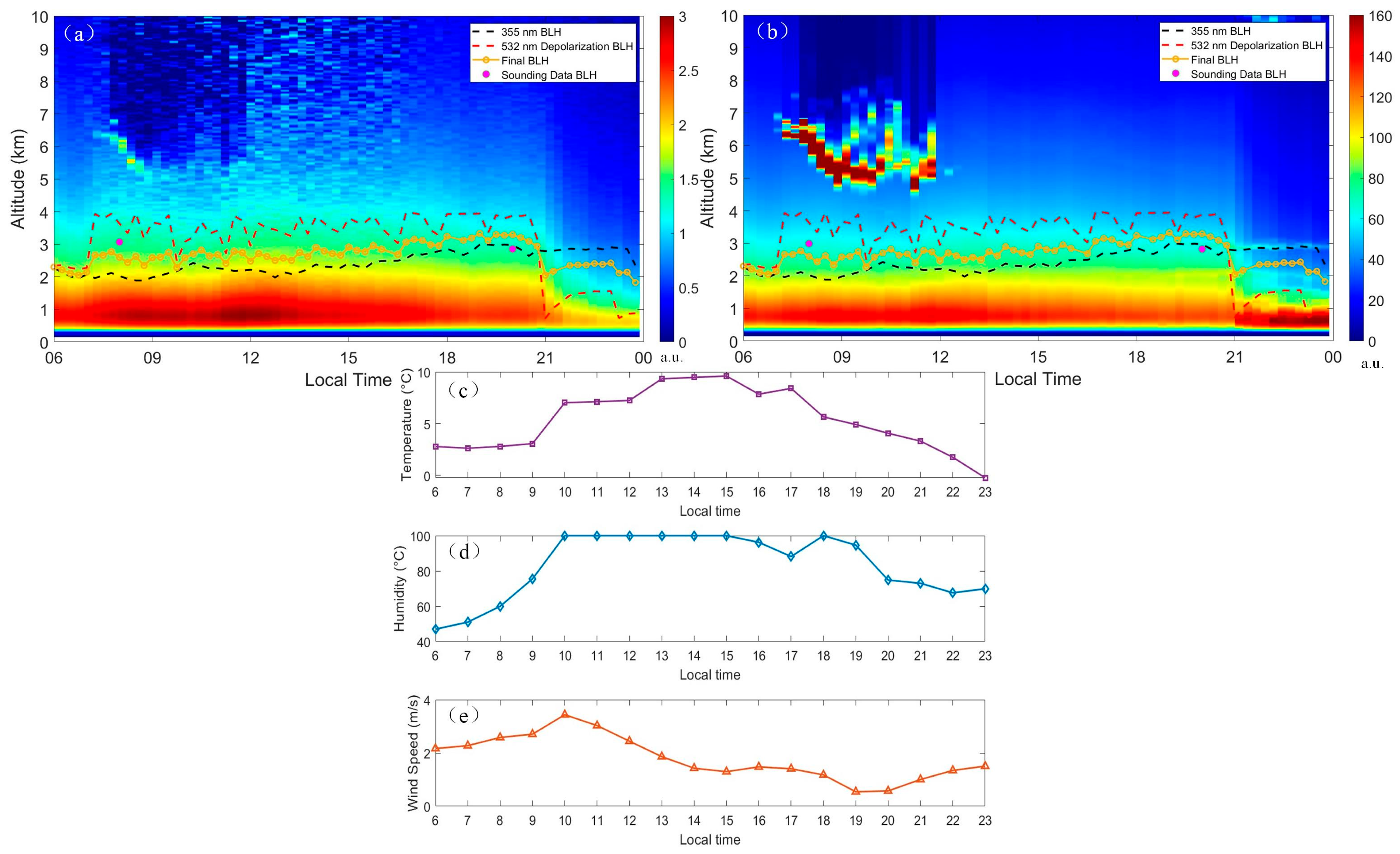
3. Results
4. Conclusions
Author Contributions
Funding
Institutional Review Board Statement
Informed Consent Statement
Data Availability Statement
Acknowledgments
Conflicts of Interest
References
- Stull, R.B. An Introduction to Boundary Layer Meteorology; Springer: Dordrecht, The Netherlands, 1988. [Google Scholar]
- Anand, M.; Pal, S. Exploring atmospheric boundary layer depth variability in frontal environments over an arid region. Bound. Layer Meteorol. 2023, 186, 251–285. [Google Scholar] [CrossRef]
- Vivone, G.; D’Amico, G.; Summa, D.; Lolli, S.; Amodeo, A.; Bortoli, D.; Pappalardo, G. Atmospheric boundary layer height estimation from aerosol lidar: A new approach based on morphological image processing techniques. Atmos. Chem. Phys. 2021, 21, 4249–4265. [Google Scholar] [CrossRef]
- Fang, Z.; Yang, H.; Cao, Y. Study of Persistent Pollution in Hefei during Winter revealed by Ground-based LiDAR and the CALIPSO Satellite. Sustainability 2021, 13, 875. [Google Scholar] [CrossRef]
- Chu, Y.; Alshammari, M.; Wang, X.; Han, M. Angle-Tunable Method for Optimizing Rear Reflectance in Fabry–Perot Interferometers and Its Application in Fiber-Optic Ultrasound Sensing. Photonics 2024, 11, 1100. [Google Scholar] [CrossRef]
- Su, T.; Li, J.; Li, C.; Xiang, P.; Lau, A.; Guo, J.; Yang, D.; Miao, Y. An intercomparison of long-term planetary boundary layer heights retrieved from CALIPSO, ground-based lidar, and radiosonde measurements over Hong Kong. J. Geophys. Res. Atmos. 2017, 122, 3929–3943. [Google Scholar] [CrossRef]
- Melfi, S.H.; Spinhirne, J.D.; Chou, S.-H.; Palm, S.P. Lidar Observations of Vertically Organized Convection in the Planetary Boundary Layer over the Ocean. J. Clim. Appl. Meteorol. 1985, 24, 806–821. [Google Scholar] [CrossRef]
- Banakh, V.A.; Smalikho, I.N.; Falits, A.V. Wind–Temperature Regime andWind Turbulence in a Stable Boundary Layer of the Atmosphere: Case Study. Remote Sens. 2020, 12, 955. [Google Scholar] [CrossRef]
- Shi, L.; Zhu, A.; Huang, L.; Yaluk, E.; Gu, Y.; Wang, Y.; Wang, S.; Chan, A.; Li, L. Impact of the planetary boundary layer on air quality simulations over the Yangtze River Delta region, China. Atmos. Environ. 2021, 263, 118685. [Google Scholar] [CrossRef]
- Li, C.; Li, J.; Dubovik, O.; Zeng, Z.C.; Yung, Y.L. Remote sensing impact of aerosol vertical distribution on aerosol optical depth retrieval from passive satellite sensors. Remote Sens. 2020, 12, 1524. [Google Scholar] [CrossRef]
- Wood, R.; Bretherton, C.S. Boundary layer depth, entrainment, and decoupling in the cloud-capped subtropical and tropical marine boundary layer. J. Clim. 2024, 17, 3576–3588. [Google Scholar] [CrossRef]
- Vakkari, V.; Baars, H.; Bohlmann, S.; Bühl, J.; Komppula, M.; Mamouri, R.E.; O’Connor, E.J. Aerosol particle depolarization ratio at 1565 nm measured with a Halo Doppler lidar. Atmos. Chem. Phys. 2021, 21, 5807–5820. [Google Scholar] [CrossRef]
- Clark, N.E.; Pal, S.; Lee, T.R. Empirical evidence for the frontal modification of atmospheric boundary layer depth variability over land. J. Appl. Meteor. Climatol. 2022, 61, 1041–1063. [Google Scholar] [CrossRef]
- Chu, Y.; Wang, Z.; Xue, L.; Deng, M.; Lin, G.; Xie, H.; Wang, Y. Characterizing warm atmospheric boundary layer over land by combining Raman and Doppler lidar measurements. Opt. Express 2022, 30, 11892–11911. [Google Scholar] [CrossRef] [PubMed]
- Peerrone, M.R.; Lorusso, A.; Romano, S. Diurnal and nocturnal aerosol properties by AERONET sun-sky-lunar photometer measurements along four years. Atmos. Res. 2022, 265, 105889. [Google Scholar] [CrossRef]
- Yang, H.; Qiu, D.; Fang, Z. LiDAR technology and experimental research for comprehensive measurement of atmospheric transmittance, turbulence, and wind. J. Appl. Remote Sens. 2024, 18, 12. [Google Scholar] [CrossRef]
- Degnan, J.J. Evolution of Single Photon Lidar: From Satellite Laser Ranging to Airborne Experiments to ICESat-2. Photonics 2024, 11, 924. [Google Scholar] [CrossRef]
- Chu, Y.; Lin, G.; Deng, M.; Guo, H.; Zhang, J.A. Characterizing Seasonal Variation of the Atmospheric Mixing Layer Height Using Machine Learning Approaches. Remote Sens. 2025, 17, 1399. [Google Scholar] [CrossRef]
- Yang, Y.; Zhao, C.; Wang, Y. Multi-source Data Based Investigation of Aerosol-Cloud Interaction over the North China Plain and North of the Yangtze Plain. J. Geophys. Res. Atmos. 2021, 19, 126. [Google Scholar] [CrossRef]
- Huang, Y.; Lu, X.; Fung, J.C.; Wong, D.C.; Li, Z.; Chen, Y.; Chen, W. Investigating southeast Asian biomass burning by the WRF-CMAQ two-way coupled model: Emission and direct aerosol radiative effects. Atmos. Environ. 2023, 294, 119521. [Google Scholar] [CrossRef] [PubMed]
- Azmi, S.; Sharma, M.; Nagar, P.K. NMVOC emissions and their formation into secondary organic aerosols over India using WRF-Chem model. Atmos. Environ. 2022, 287, 119254. [Google Scholar] [CrossRef]
- Bravo-Aranda, J.A.; Moreira, G.D.A.; Navas-Guzmán, F.; Granados-Muñoz, M.J.; Guerrero-Rascado, J.L.; Pozo-Vázquez, D.; Arbizu-Barrena, C.; Reyes, F.J.O.; Mallet, M.; Arboledas, L.A. A new methodology for PBL height estimations based on lidar depolarization measurements: Analysis and comparison against MWR and WRF model-based results. Atmos. Chem. Phys. 2017, 17, 6839–6851. [Google Scholar] [CrossRef]
- Li, M.; Wu, Y.; Yuan, J.; Zhao, L.; Tang, D.; Dong, J.; Xia, H.; Dou, X. Stratospheric aerosol lidar with a 300m diameter superconducting nanowire single-photon detector at 1064 nm. Opt. Express 2023, 31, 2768–2779. [Google Scholar] [CrossRef] [PubMed]
- Liu, X.; Zhang, L.; Zhai, X.; Li, L.; Zhou, Q.; Chen, X.; Li, X. Polarization Lidar: Principles and Applications. Photonics 2023, 10, 1118. [Google Scholar] [CrossRef]
- Dai, G.; Wang, X.; Sun, K.; Wu, S.; Song, X.; Li, R.; Yin, J.; Wang, X. Calibration and retrieval of aerosol optical properties measured with Coherent Doppler Lidar. J. Atmos. Ocean Technol. 2021, 38, 1035–1045. [Google Scholar] [CrossRef]
- Gong, W.; Zhang, J.; Mao, F.; Li, J. Measurements for profiles of aerosol extinction coeffcient, backscatter coeffcient, and lidar ratio over Wuhan in China with Raman/Mie lidar. Chin. Opt. Lett. 2010, 8, 533–536. [Google Scholar] [CrossRef]
- Mallat, S.; Hwang, W. Singularity detection and processing with wavelets. IEEE Trans. Inf. Theory 1992, 38, 617–643. [Google Scholar] [CrossRef]
- Morille, Y.; Haeffelin, M.; Drobinski, P.; Pelon, J. STRAT: An Automated Algorithm to Retrieve the Vertical Structure of the Atmosphere from Single-Channel Lidar Data. J. Atmos. Ocean. Technol. 2007, 24, 761–775. [Google Scholar] [CrossRef]
- Zhou, T.; Huang, J.; Huang, Z.; Liu, J.; Wang, W.; Lin, L. The depolarization–attenuated backscatter relationship for dust plumes. Opt. Express 2013, 21, 15195–15204. [Google Scholar] [CrossRef] [PubMed]
- Hersbach, H.; Bell, B.; Berrisford, P.; Biavati, G.; Horányi, A.; Muñoz Sabater, J.; Nicolas, J.; Peubey, C.; Radu, R.; Rozum, I.; et al. ERA5 Hourly Data on Single Levels from 1940 to Present. Copernicus Climate Change Service (C3S). 2023. Available online: https://cds.climate.copernicus.eu/datasets/reanalysis-era5-single-levels?tab=overview (accessed on 9 September 2023).
- Shi, H.; Cao, X.; Li, Q.; Li, D.; Sun, J.; You, Z.; Sun, Q. Evaluating the Accuracy of ERA5 Wave Reanalysis in the Water Around China. J. Ocean Univ. China 2021, 20, 1–9. [Google Scholar] [CrossRef]
- Sharmar, V.; Markina, M. Validation of global wind wave hindcasts using ERA5, MERRA2, ERA-Interim and CFSRv2 reanalyzes. IOP Conf. Ser. Earth Environ. Sci. 2020, 606, 012056. [Google Scholar] [CrossRef]
- Fernald, F.G. Analysis of Atmospheric Lidar Observation: Some Comments. Appl.Opt. 1984, 23, 652–653. [Google Scholar] [CrossRef] [PubMed]
- Vogelezang, D.H.P.; Holtslag, A.A.M. Evaluation and model impacts of alternative boundary-layer height formulations. Bound.-Layer Meteorol. 1996, 81, 245–269. [Google Scholar] [CrossRef]
- Seidel, D.J.; Zhang, Y.; Beljaars, A.; Golaz, J.-C.; Jacobson, A.R.; Medeiros, B. Climatology of the planetary boundary layer over the continental United States and Europe. J. Geophys. Res. Atmos. 2012, 117, D17106. [Google Scholar] [CrossRef]
- Guo, J.; Miao, Y.; Zhang, Y.; Liu, H.; Li, Z.; Zhang, W.; He, J.; Lou, M.; Yan, Y.; Bian, L.; et al. The climatology of planetary boundary layer height in China derived from radiosonde and reanalysis data. Atmos. Chem. Phys. 2016, 16, 13309–13319. [Google Scholar] [CrossRef]
- Smalikho, I.N.; Banakh, V.A. Measurements of wind turbulence parameters by a 659 conically scanning coherent Doppler lidar in the atmospheric boundary layer. Atmos. Meas. Tech. 2017, 660, 4191–4208. [Google Scholar] [CrossRef]


| Technical Indicator | Parameter |
|---|---|
| Laser type | Nd:YAG |
| Laser wavelength/nm | 355, 532 |
| Receive channel | 355 nm, 532 nm ||, 532 nm ⊥ |
| Pulse energy/mJ | 50,90 |
| Pulse width/ns | 20 |
| Repetition rate/Hz | 20 |
| Receiving Telescope/mm | 400 diameter, Cassegrain |
| Vertical resolution/m | 7.5 |
Disclaimer/Publisher’s Note: The statements, opinions and data contained in all publications are solely those of the individual author(s) and contributor(s) and not of MDPI and/or the editor(s). MDPI and/or the editor(s) disclaim responsibility for any injury to people or property resulting from any ideas, methods, instructions or products referred to in the content. |
© 2025 by the authors. Licensee MDPI, Basel, Switzerland. This article is an open access article distributed under the terms and conditions of the Creative Commons Attribution (CC BY) license (https://creativecommons.org/licenses/by/4.0/).
Share and Cite
Fang, Z.; Li, S.; Yang, H.; Kuang, Z. A Dual-Wavelength Lidar Boundary Layer Height Detection Fusion Method and Case Analysis. Photonics 2025, 12, 741. https://doi.org/10.3390/photonics12080741
Fang Z, Li S, Yang H, Kuang Z. A Dual-Wavelength Lidar Boundary Layer Height Detection Fusion Method and Case Analysis. Photonics. 2025; 12(8):741. https://doi.org/10.3390/photonics12080741
Chicago/Turabian StyleFang, Zhiyuan, Shu Li, Hao Yang, and Zhiqiang Kuang. 2025. "A Dual-Wavelength Lidar Boundary Layer Height Detection Fusion Method and Case Analysis" Photonics 12, no. 8: 741. https://doi.org/10.3390/photonics12080741
APA StyleFang, Z., Li, S., Yang, H., & Kuang, Z. (2025). A Dual-Wavelength Lidar Boundary Layer Height Detection Fusion Method and Case Analysis. Photonics, 12(8), 741. https://doi.org/10.3390/photonics12080741