Non-Destructive Discrimination and Traceability of Exocarpium Citrus grandis Aging Years via Feature-Optimized Hyperspectral Imaging and Broad Learning System

Abstract

Exocarpium Citrus grandis is a traditional Chinese medicinal and edible herb whose pharmacological efficacy is closely tied to its aging duration. The accurate discrimination of aging years is essential for quality control but remains challenging due to limitations in current analytical techniques. This study proposes a novel feature-optimized classification framework that integrates hyperspectral imaging (HSI) with a Broad Learning System (BLS). Bilateral spectral data (side A and side B) were collected to capture more comprehensive sample information. A combination of normalization (NOR) preprocessing and the Iterative Variable Importance for Spectral Subset Selection Algorithm (iVISSA) was found to be optimal. The NOR–iVISSA–BLS model achieved classification accuracies of 94.09 ± 1.01% (side A) and 95.10 ± 0.82% (side B). Furthermore, cross-validation between the two sides (A→B: 94.92%, B→A: 94.11%) confirmed the model’s robustness and generalizability. This dual-side spectral validation strategy offers a rapid, nondestructive, and reliable solution for the vintage authentication of Exocarpium Citrus grandis, contributing to the modernization of quality control in medicinal foodstuffs.

1. Introduction

Exocarpium Citrus grandis is a traditional Chinese medicinal herb widely used in both medicine and functional food. Its efficacy in relieving cough, resolving phlegm, and regulating qi is closely associated with its storage duration [1]. As the storage time increases, biochemical conversions such as the hydrolysis of flavonoids and the evolution of volatile compounds occur [2,3]. Consequently, the aging year becomes a critical quality indicator. However, the deliberate mislabeling of younger samples as aged ones disrupts market integrity and poses safety risks to consumers.

At present, the identification of the vintage of Exocarpium Citrus grandis mainly relies on sensory evaluation and chemical analysis methods, such as high-performance liquid chromatography (HPLC) and gas chromatography–mass spectrometry (GC-MS) [4]. However, these traditional means have many limitations: high subjectivity, poor reproducibility, high sample destructiveness, and long testing periods. These problems have seriously restricted the accurate evaluation of the quality of Exocarpium Citrus grandis herbs and affected the efficiency of market distribution. Therefore, there is an urgent need to develop a rapid, nondestructive, and accurate method to identify the vintage of Exocarpium Citrus grandis in order to improve the quality control level of Exocarpium Citrus grandis and regulate the market circulation order.

Hyperspectral imaging (HSI) technology combines spectroscopy and computer vision to acquire spectral information from each pixel of a sample image, resulting in a three-dimensional data structure with spatial (x, y) and spectral dimensions, often referred to as a “hypercube” [5]. This comprehensive approach to data acquisition allows HSI to deeply analyze the chemical, physical, and geometric properties of substances and has led to a wide range of applications in quality testing [6,7]. In contrast, techniques like Raman spectroscopy and Fourier-transform infrared (FTIR) spectroscopy acquire data from single points, providing molecular-level insights but lacking the spatial resolution of HSI. This makes HSI particularly advantageous when high-throughput, non-destructive testing is required as it captures comprehensive data across large areas in a single scan. Such capabilities make HSI particularly suitable for quality control in various industries, where the need for detailed, spatially resolved analysis is crucial. For instance, HSI has been successfully applied in the quality testing of meat (e.g., salmon), fruits (e.g., strawberries), and Chinese herbs (e.g., Radix Paeoniae Alba), showcasing its ability to provide both chemical and spatial information in a non-invasive manner [8,9,10]. With the rapid development of machine learning, especially deep learning, more and more studies are applying it to the analysis of hyperspectral data. Chen et al. combined hyperspectral imaging with a fully connected neural network to successfully realize the identification of the growth year of ginseng [11]; Hu et al. combined hyperspectral images and a one-dimensional convolutional neural network (CNN) to efficiently classify Chuanbeimu [12]; and Wang et al. combined hyperspectral imaging with a temporal convolutional network attentional mechanism (TCNA) to achieve the accurate prediction of the content of six rare ginseng saponins (RGs) with a model coefficient of determination (R²) of more than 0.89. These studies provide an important reference for the application of hyperspectral imaging in the quality inspection of medicinal plants [13]. However, although deep learning performs well in hyperspectral data analysis, its demand for large-scale labeled data and computational resources makes its generalization in certain applications challenging.

The Broad Learning System (BLS) is a shallow, incremental learning framework that optimizes model performance by expanding the network width rather than increasing its depth [14]. This architecture significantly reduces computational complexity while maintaining high accuracy, making it particularly suitable for scenarios involving limited data. Compared to traditional deep learning models, BLS demonstrates superior generalization and robustness in small-sample tasks due to its simplified structure and fast training efficiency [15]. Recent studies have begun integrating the BLS with spectral technologies for agricultural quality assessment. For instance, Li et al. successfully predicted the soluble solids content (SSC) of loquat using breadth learning combined with near-infrared spectroscopy (NIR) with a coefficient of determination (R²) of 0.8646 [16], while Zhu et al. predicted the catechin content of black tea by combining hyperspectral imaging with the BLS [17]. These studies highlight the potential of the BLS in spectral-based analysis. However, most HSI-based studies in medicinal herbs still rely on single-sided spectral acquisition and deep learning models, which require large datasets and high computational costs. In contrast, the BLS offers an efficient and generalizable alternative for small-sample learning. Yet, its application in hyperspectral classification—particularly for aging-year discrimination in traditional Chinese herbs like Exocarpium Citrus grandis—remains underexplored. This study addresses this gap by proposing a feature-optimized, dual-view BLS framework for nondestructive vintage identification.

Although hyperspectral imaging (HSI) has been widely applied in the quality inspection of traditional Chinese medicine, most existing studies rely on spectral data collected from only one side of the sample. However, due to natural variability in internal structure and surface composition, the spectral characteristics of different sides may vary significantly. Models based solely on single-sided data may thus face limitations in generalizability and robustness. In this study, we systematically explored the integration of existing techniques to improve classification performance for Exocarpium Citrus grandis. Specifically, (1) hyperspectral data were acquired from both sides (A and B) of the samples to capture more complete spectral information, (2) multiple algorithms were evaluated and compared individually on each side, (3) cross-side mutual validation was conducted to assess model stability and generalization, and (4) the Broad Learning System (BLS) was applied, which offers efficient learning in small-sample settings.

2. Materials and Methods

2.1. Sample Presentation

This study used commercially available dried sliced tangerine peel samples from four different years. The sample variety was Jinmao, produced in Huazhou, Maoming City, Guangdong Province, China. The sample years were 2011, 2015, 2019, and 2023 and the number of samples was 128, 122, 121, and 122, respectively. The thickness of the samples in each year was 2.43 ± 0.13 mm in 2011, 2.37 ± 0.12 mm in 2015, 2.44 ± 0.13 mm in 2019, and 2.43 ± 0.14 mm in 2023. This design allowed for both trend exploration and preliminary model validation while controlling for sample imbalance and external variation. All samples were stored under sealed conditions in ambient, room-temperature storage in Maoming, Guangdong, with no exposure to light. This consistent storage method minimized variability due to environmental factors.

2.2. Hyperspectral Image Acquisition and Spectral Extraction

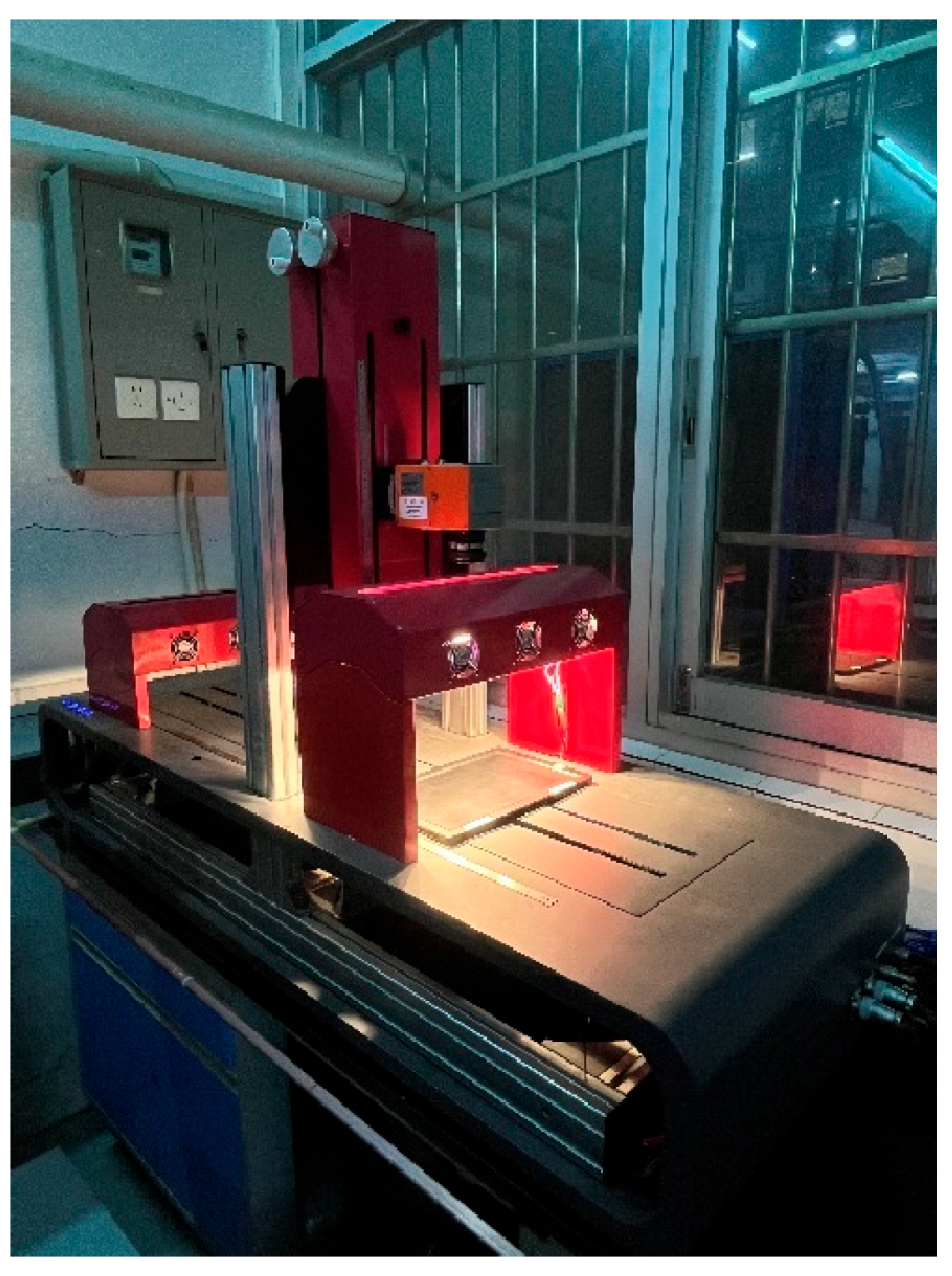
In this experiment, a short-wave near-infrared hyperspectral imaging system (SWIR-HSI, 935.61–1720.23 nm) was used. The system consisted of a dark box, a hyperspectral imager (Specim FX17, Specim, Spectral Imaging Ltd., Oulu, Finland), a set of 280 W halogen lamps (DECOSTAR 51S, Osram Corp., Munich, Germany), a mobile platform (HXY-OFX01, Red Star Yang Technology Corp., Wuhan, China), and image acquisition software (Lumo-Scanner, 2019); the system configuration is shown in Figure 1. When operating the SWIR-HSI, the moving speed of the platform was set at 7.5 mm/s, the exposure time of the spectrometer was 3.2 ms, the distance between the lens and the sample was kept at 32 cm to ensure the image quality, and the detection wavelength range was from 935.61 nm to 1720.23 nm with a wavelength interval of 1.67 nm.

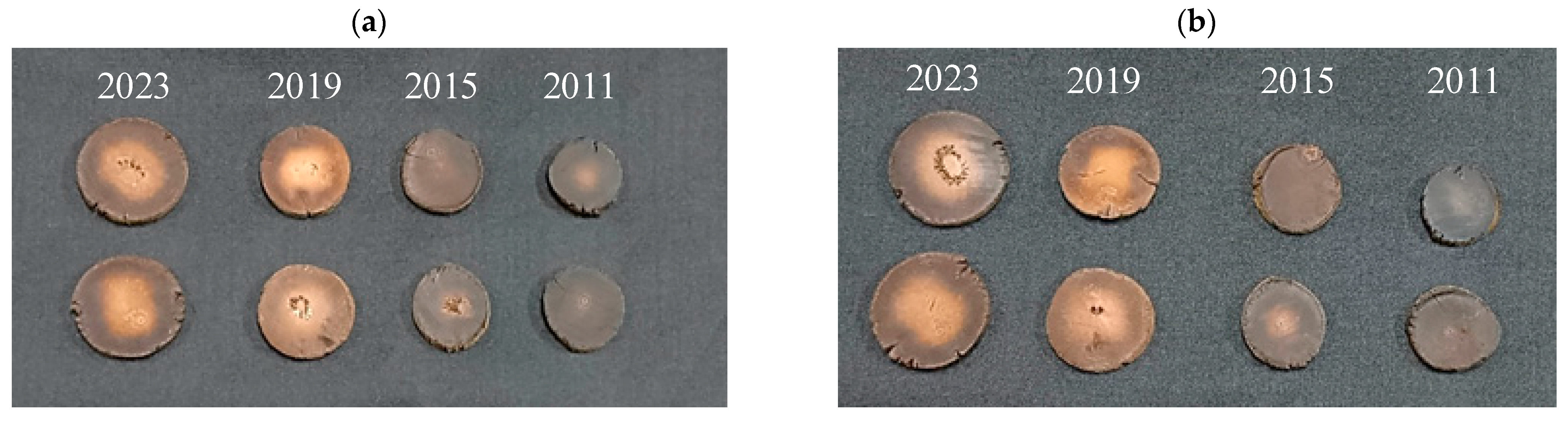
In the spectral acquisition process, the hyperspectral image acquisition and analysis of the sample adopted a two-sided detection process: Firstly, the hyperspectral image acquisition and data analysis were carried out on the A-side of the sample and then the sample was flipped 180° along the central axis, and measurements were taken on the B-side under the same parameter conditions for comparative analysis. After completing the acquisition of the hyperspectral image, it was necessary to use the blackboard reference image ($I_B$) and the whiteboard reference image ($I_W$) to perform the black and white correction of the acquired original image by the correction algorithm, as shown in Equation (1):

$$R_c={\displaystyle \frac{R_{raw}-I_B}{I_W-I_B}}$$

(1)

where $R_c$ is the corrected reflectance image and $R_{raw}$ is the original reflectance image. A sample example is shown in Figure 2.

After the spectral data collection was completed, the whole area of the Exocarpium Citri Grandis samples was selected as the region of interest and the average spectrum of the region was calculated. For the four years of Exocarpium Citri Grandi samples, a total of 493 spectral data were extracted. Subsequently, the data were processed using the Kennard–Stone (K–S) algorithm, which divided the data in order of sample year and divided the data into training and test sets at a ratio of 7:3. Finally, 345 training set samples and 148 test set samples were obtained.

2.3. Determination of Flavonoids

For each year, 6 groups of samples, each weighing approximately 30 g (total of 24 groups), were randomly selected. The Hua Ju Hong samples were ground and sieved through a No. 4 sieve. Total flavonoid content was determined following the method described in DB4409/T 06-2019, a local standard published in Guangdong Province, China. About 0.2 g of dried sample powder was extracted using Soxhlet extraction. After extraction, the solution was cooled, transferred, and diluted to the required volume. Naringin, dried to a constant weight, was used as a reference. The absorbance at 384 nm was measured using a UV–visible spectrophotometer and a standard curve was constructed. A 2 mL aliquot of the test solution was taken and the absorbance was measured. The total flavonoid content was calculated using the regression equation. The total flavonoid content was calculated using the following formula:

$$X={\displaystyle \frac{A\times V_2}{V_1\times M\times \left(1-m\right)\times 1000}}\times 100\%$$

(2)

where X is total flavonoid content in the sample (g/100 g), $A$ is the flavonoid amount in the test solution derived from the standard curve (mg), $M$ is the sample mass (g), $V_1$ is the volume of the test sample (mL), $V_2$ is the total volume of the sample solution (mL), and $m$ is the moisture content.

2.4. Principal Component Analysis

Principal Component Analysis (PCA) is a statistical technique used to reduce the dimensionality of high-dimensional data by transforming the original variables into a new set of variables, called principal components. These components are ordered such that the first few components capture most of the variance in the data, thereby retaining the most important features while discarding less informative ones. PCA achieves this by identifying linear combinations of the original variables that maximize the variance, allowing the data to be represented in fewer dimensions without losing significant information.

2.5. Pre-Processing Methods

In order to eliminate the influence of noise, this study used four preprocessing methods to process the spectral data, including Savitzky–Golay smoothing (SG), normalization (NOR), baseline correction (BL), and standard normal variate transformation (SNV). Among them, SG smoothing reduces the influence of high-frequency noise by smoothing spectral data and improves signal quality; NOR adjusts the spectral data to the same scale to eliminate the influence caused by the difference in light intensity between samples; BL removes the baseline drift in a spectrum to make the starting and ending points of the spectrum consistent; SNV eliminates the scattering effect and standardizes the mean and variance of each spectrum, thereby reducing the deviation between spectra and improving the consistency of data [18].

The volatile oil content was determined according to DB4409/T 06-2019, using Method A of the volatile oil determination protocol. Three groups were randomly selected for each gradient and tested at 30 g per group.

2.6. Feature Extraction Methods

Hyperspectral data has high-dimensional characteristics. SWIR contains 224 characteristic bands, some of which are redundant and can affect the performance of a model. Therefore, this study used three feature extraction methods: competitive adaptive reweighted sampling (CARS), the successive projective algorithm (SPA), and the Iterative Variable Importance for Spectral Subset Selection Algorithm (iVISSA) to select characteristic wavelengths.

CARS employs a competitive adaptive reweighting strategy, which iteratively adjusts the weights of spectral bands to prioritize those most relevant to the target variable while eliminating redundant ones [19]. This not only enhances model performance but also alleviates the computational burden associated with high-dimensional data. In contrast, SPA operates by evaluating the contribution of each spectral band to the overall spectral variance, selecting bands that maximize the diversity of the feature space [20]. This approach strengthens the discriminative capability of the selected features, improving prediction accuracy and mitigating overfitting. Meanwhile, iVISSA takes an iterative approach to rank the importance of each spectral band in relation to the specific classification or regression task [21]. By progressively selecting the most significant features and minimizing redundancy, iVISSA ensures that only the most informative wavelengths are retained, optimizing model performance.

2.7. Model Algorithm and Model Evaluation

2.7.1. Model Comparison Algorithms

Partial Least Squares Discriminant Analysis (PLS-DA) is a supervised learning method based on the partial least squares regression model [22]. It projects data into the latent variable space, maximizes inter-class differences, and minimizes intra-class differences, thereby achieving data classification. Its core idea is to map high-dimensional data to a low-dimensional space and construct a classification model by linearly combining the latent variables.

Random Forest (RF) is an integrated learning method that performs classification or regression by constructing multiple decision trees [23]. During the training process, RF constructs each tree on a random subset of the data and eventually integrates the predictions of multiple trees by voting to output the final classification results. The generation process of each tree is independent, so RF has strong resistance to overfitting.

Convolutional Neural Network (CNN) is a deep learning model mainly used to process spatial structural features in data [24]. The CNN architecture used in this study consisted of three convolutional layers followed by a fully connected layer and an output layer. The input layer accepted one-dimensional hyperspectral data with a single channel. The first convolutional layer (CONV1) applied 64 filters with a kernel size of 9 and a stride of 1, using ReLU activation, followed by MaxPooling with a kernel size of 3 and a stride of 1. The second convolutional layer (CONV2) reduced the number of channels to 32, with a kernel size of 7 and a stride of 1, and was followed by ReLU activation and MaxPooling with the same kernel and stride. The third convolutional layer (CONV3) further reduced the number of channels to 16, using a kernel size of 5 and a stride of 1, followed by ReLU activation and MaxPooling. The output of the convolutional layers was then flattened and passed through a fully connected layer (fc) with 64 nodes. Finally, the output layer consisted of 4 neurons for classification, with a softmax activation function to compute the final class probabilities. The model was optimized using the Adam optimizer with a learning rate of 0.001.

2.7.2. Broad Learning System

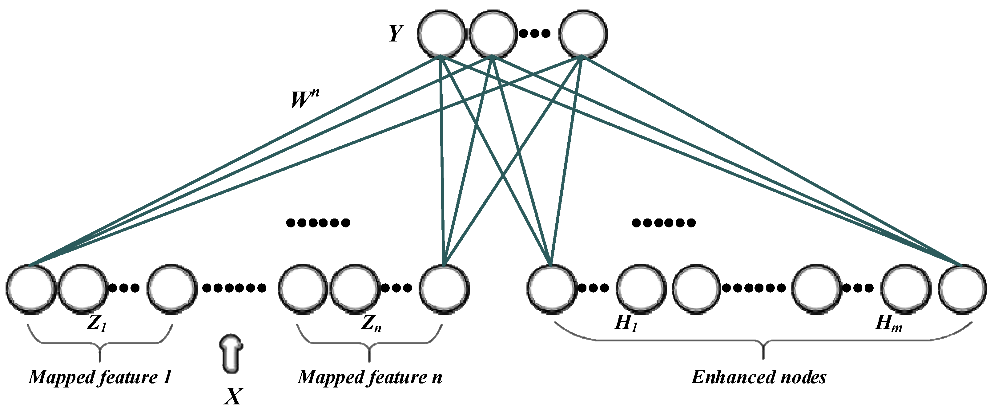
The Broad Learning System (BLS) is a shallow learning framework based on Random Vector Functional-Link (RVFL), which achieves efficient learning by expanding feature nodes horizontally in a single-layer network (instead of stacking multiple hidden layers). Its model structure is shown in Figure 3, and the method consists of an input layer, a mapping feature layer, and an augmentation node layer.

In the BLS, the input data $X$ is first mapped to the feature space by a set of mapping functions f, generating multiple mapped features $Z_1$, $Z_2$, …, $Z_n$. Each mapped feature $Z_i$ is obtained by applying a nonlinear activation function to a linear combination of the input data and the mapped weights, as shown in Equation 3:

$$Z_i={\varphi }_i\left(W_{i}X+{\beta }_i\right), i=\mathrm{1,2},\dots ,n$$

(3)

where $W_i$ is the mapping weight, ${\beta }_i$ is the bias term, and ${\varphi }_i$ is the nonlinear activation function Sigmoid.

Next, these mapped features are combined through the augmentation node layer. Augmentation nodes H₁, H₂, …, H_m form a new feature representation H:

$$H_m={\xi }_j\left(Z^n{W}_j+{\beta }_j\right), j=\mathrm{1,2},\dots ,n$$

(4)

where $W_j$ is the weight matrix of the augmented node, ${\beta }_j$ is the bias term of the augmented node, and ${\xi }_j$ is the activation function.

Finally, the feature nodes Z_n and H_m augmentation nodes are connected and linearly transformed to obtain the final output $Y$:

$$Y=\left[Z_1,Z_2,\dots ,Z_n,H_1,H_2,\dots ,H_m\right]W^o$$

(5)

where $W^o$ is the weight matrix of the connected output layer. Its computation is performed by the least squares method. Assuming that A = [Z_n|H_m] and that the category labelling matrix $Y$ is known, the weights are calculated as

$$W^o=A^{-1}Y$$

(6)

For the BLS model, the number of mapping nodes and enhancement nodes was set to 50 for both, optimizing the feature learning and enhancing the model’s generalization capability.

2.7.3. Model Evaluation

In this study, a confusion matrix was employed as a standard evaluation tool to assess the classification performance of the models. It summarized the number of correct and incorrect predictions by comparing actual and predicted classes and consisted of four fundamental components: true positives (TPs), false positives (FPs), true negatives (TNs), and false negatives (FNs). Based on these values, four commonly used metrics were calculated: accuracy, precision, recall, and F1-score, as shown in Equations (7)–(10). These metrics comprehensively reflected the effectiveness and robustness of the classification models.

$$Accuracy(\%)={\displaystyle \frac{TP+TN}{TP+FN+FP+TN}}$$

(7)

$$Precision(\%)={\displaystyle \frac{TP}{TP+FP}}$$

(8)

$$Recall(\%)={\displaystyle \frac{TP}{TP+FN}}$$

(9)

$$F1-Score(\%)={\displaystyle \frac{2\ast Precision\ast Recall}{Precision+Recall}}$$

(10)

3. Results

3.1. Flavonoid Content Analysis

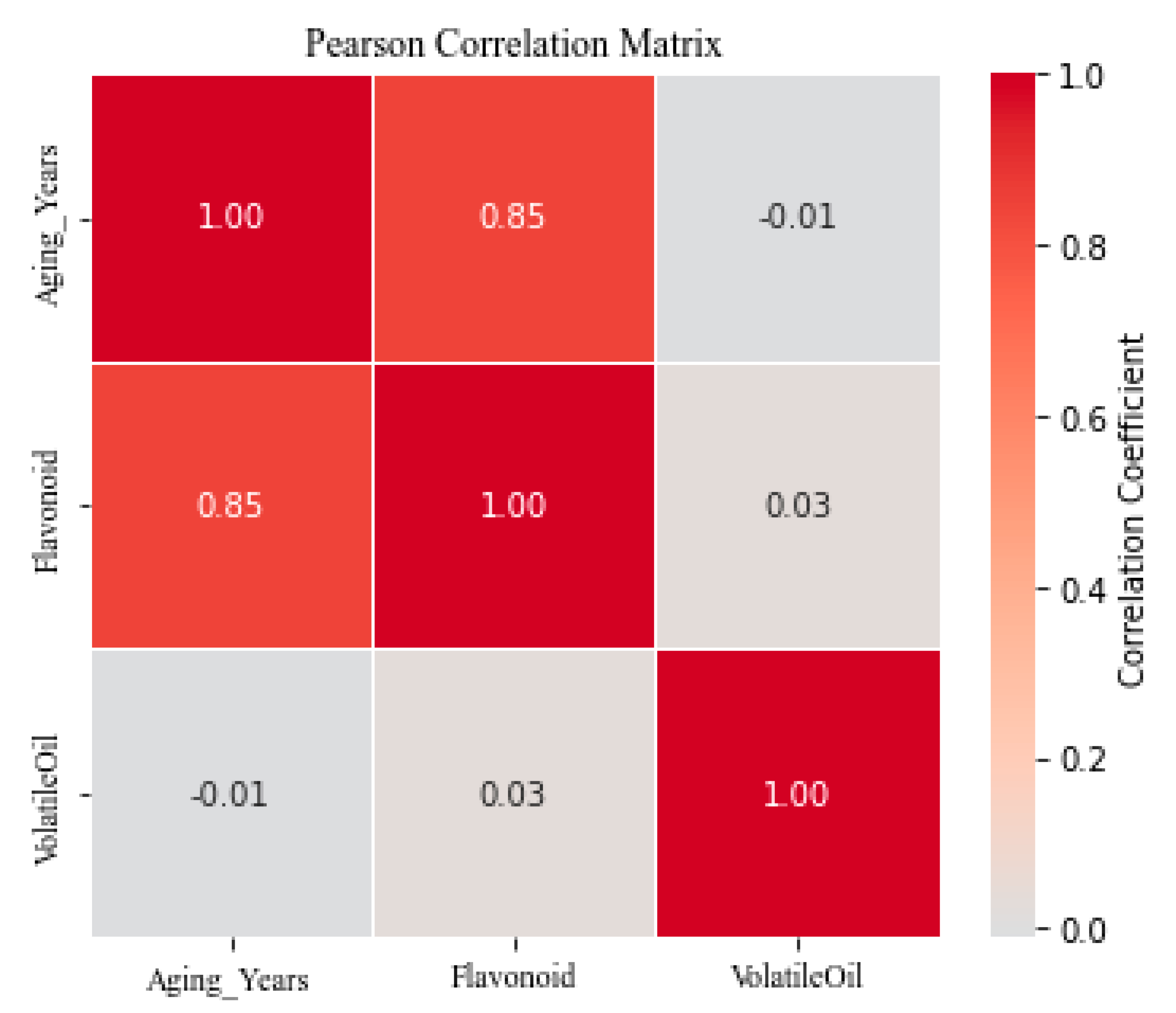
The test results of different aged Exocarpium Citrus grandis samples showed that the contents of both total flavonoids and volatile oils exhibited a ‘first increasing and then decreasing’ trend with aging time (

Table 1. Standard error analysis of flavonoid content and volatile oil (mean ± std).

Parameter	2023	2019	2015	2011
Flavonoid content (%)	0.5986 ± 0.2418 d	0.6506 ± 0.2133 c	0.7433 ± 0.1325 a	0.7075 ± 0.0833 b
Volatile oil (ml/30 g)	0.0700 ± 0.1732 c	0.2000 ± 0.0200 a	0.1067 ± 0.0156 b	0.1000 ± 0.00 b

Note: Different letters indicate a significant difference (p < 0.05); the same letter indicates no significant difference (p > 0.05). The values are given with means ± standard deviations.

). Specifically, for flavonoids, the contents were 0.5986 ± 0.2418% (2 years), 0.6506 ± 0.2133% (6 years), 0.7433 ± 0.1325% (10 years), and 0.7075 ± 0.0833% (14 years), while, for volatile oils, the contents were 0.0700 ± 0.1732 mL, 0.2000 ± 0.0200 mL, 0.1067 ± 0.0156 mL, and 0.1000 ± 0.0000 mL, respectively. This dynamic change may be attributed to a series of complex chemical transformation reactions during the aging process [25]. A Pearson correlation analysis (Figure 4) further supported these findings, revealing a strong positive linear correlation between aging year and total flavonoid content (r = 0.851), whereas no significant correlation was found between aging year and volatile oil content (r = −0.008), indicating distinct and potentially non-linear transformation mechanisms.

In the early stage of storage, flavonoid glycosides are gradually hydrolyzed to flavonoid aglycones under the action of endogenous enzymes. Meanwhile, suitable temperature and humidity conditions limit further degradation, thereby promoting the accumulation of total flavonoids. During the aging period of 10 to 14 years, a slight decrease in flavonoid content was observed, which could be attributed to the declining structural stability of flavonoids caused by oxidation, low-level hydrolysis, or environmental fluctuations such as humidity and temperature changes during long-term storage [26]. Although previous studies have suggested that microbial activity or environmental fluctuations may influence flavonoid content [27], in this study, all samples were stored under controlled and consistent sealed conditions, minimizing the possibility of storage-induced variability. Therefore, the observed fluctuations were more likely due to the intrinsic chemical transformation during aging rather than external microbial or environmental effects.

Changes in volatile oil content also showed an apparent “increase-then-decrease” trend with aging time; however, Pearson correlation analysis indicated no significant linear relationship between volatile oil content and storage year (r = −0.008), suggesting that this was a non-monotonic process influenced by multiple factors. To explore this relationship more accurately, we performed Spearman rank correlation analysis, which revealed a weak negative correlation (r = −0.20), further confirming the non-linear nature of this trend. Similarly, flavonoid content showed a significant correlation with storage year. Pearson correlation analysis indicated a strong positive correlation between flavonoid content and storage year (r = 0.85), suggesting a linear relationship. However, Spearman rank correlation analysis also showed a strong negative correlation (r = −0.80), indicating that the relationship between flavonoid content and aging was non-monotonic. These results highlight the non-monotonic nature of both volatile oil content and flavonoid content changes. While Pearson correlation captured the strong positive relationship between flavonoid content and storage year, Spearman rank correlation better captured the non-monotonic variations in both volatile oil and flavonoid contents. Therefore, non-linear correlation metrics, such as Spearman, provided a more accurate representation of the data.

3.2. Spectral Analysis

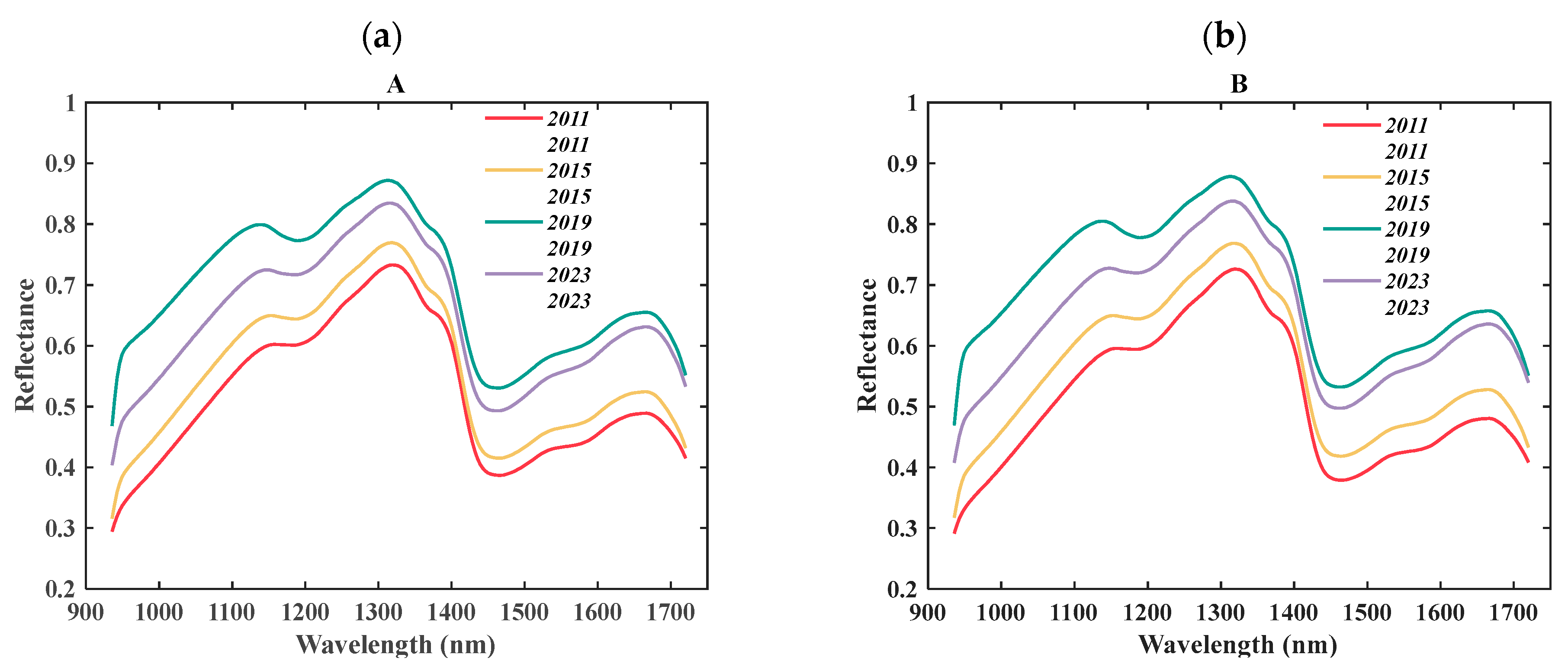
Figure 5 shows that the average spectral reflectance of Exocarpium Citrus grandis samples across different aging years followed a “first increasing and then decreasing” trend, and the spectral differences between surface A and surface B were relatively minor. In the characteristic absorption bands, the peak near 1200 nm was primarily attributed to the first overtone of C–H stretching vibrations [28]; the absorption in the 1300 nm region was likely due to the combination band of O–H and C–H vibrations, reflecting the coordinated evolution of hydroxyl (–OH) and alkyl structures during aging [10]. The 1450 nm band corresponded to O–H and N–H bending vibrations, which are commonly associated with moisture content and phenolic hydroxyl groups in flavonoids and amine-containing volatiles. The 1680 nm peak arose from the first overtone of O–H stretching, which was highly sensitive to flavonoid aglycones and phenolic compounds, and its intensity was indicative of hydroxyl accumulation or loss [29]. In the early stage of aging, low reflectance was observed, likely due to the dense cellular structure and insufficient hydrolysis of internal components. As aging progressed, glycosidic bonds were cleaved, free hydroxyl groups accumulated, and microporous structures formed, resulting in increased reflectivity. This period also corresponded to the peak accumulation of flavonoids and volatile oils. In the later stage, the degradation of bioactive compounds, collapse of pore structures, and redistribution or volatilization of moisture contributed to a decline in reflectance, consistent with the decrease in key component concentrations [30]. The overall spectral change trend was consistent with the “first increase and then decrease” pattern of flavonoid content. These variations in reflectance between sides A and B likely reflected the differing distributions of chemical constituents across the sample surfaces, with the outer peel being richer in flavonoids and volatile oils.

3.3. PCA

PCA was performed on the spectral data of side A and side B, and the results are shown in Figure 4. For side A, the principal components PC-1, PC-2, and PC-3 explained 92.40%, 6.89%, and 0.42% of the data variance, respectively, with a cumulative contribution rate of 99.71%; for side B, the principal components PC-1, PC-2, and PC-3 explained 92.89%, 6.46%, and 0.38% of the data variance, respectively, with a cumulative contribution rate of 99.73%. From the clustering trend of sides A and B, the two showed similar distribution patterns, indicating that the spectral characteristics of both side A and side B changed consistently between years. Specifically, as the aging years of Exocarpium Citri grandis increased, its spectral characteristics changed significantly, and this trend was consistent with the change in the average spectral curve in Figure 5, showing the gradual change in the spectral response of Exocarpium Citri grandis samples of different years. In Figure 6, the samples from 2011 and 2015 were clustered more closely, indicating that the spectral characteristics between these two years were similar, while the samples from 2019 and 2023 showed greater dispersion, indicating that the spectral characteristics of the samples in these years changed significantly. This result further verifies that the spectral characteristics of Exocarpium Citri grandis vary significantly between years, and this changing trend is closely related to the transformation process of flavonoids.

3.4. Full Wavelength Modeling

In this study, four models, PLS-DA, RF, CNN, and BLS, were used to model the full-band hyperspectral data of the front and back sides (side A and side B) of the Exocarpium Citri grandis, respectively, and the effects of different preprocessing methods (Raw, SG, SNV, NOR, BL) on the performance of the models were discussed. The specific results are presented in

Table 2. Classification results of PLS-DA, RF, CNN, and BLS models based on full-spectra data from side A.

Model	Pretreatment	Accuracy (%)	Precision (%)	Recall (%)	F1-Score (%)
PLS-DA	Raw	87.84	88.84	87.84	87.35
	SG	87.16	87.92	87.16	86.72
	NOR	88.51	89.94	88.49	88.00
	BL	85.81	88.51	85.81	84.72
	SNV	89.19	90.56	89.21	88.79
RF	Raw	86.49	88.69	86.47	86.06
	SG	84.46	85.91	84.42	83.88
	NOR	86.49	88.86	86.47	85.66
	BL	80.41	81.49	80.37	80.07
	SNV	89.19	91.95	89.19	88.74
CNN	Raw	87.84 ± 0.95	92.29	91.89	92.01
	SG	88.65 ± 1.0	93.19	91.89	91.72
	NOR	90.4 ± 1.0	91.63	90.66	90.78
	BL	88.11 ± 0.6	92.25	91.18	91.13
	SNV	92.57 ± 0.82	93.24	93.30	93.21
BLS	Raw	90.81 ± 0.6	93.04	91.20	90.97
	SG	91.62 ± 0.37	92.60	91.93	91.80
	NOR	93.65 ± 0.9	95.65	94.58	94.65
	BL	90.81 ± 1.02	92.29	91.91	91.77
	SNV	90.13 ± 0.6	91.27	90.52	90.56

Note: Precision, recall, and F1-score were calculated based on the best-performing model, and the CNN and BLS achieved the highest accuracy based on five independent repeated experiments.

and

Table 3. Classification results of PLS-DA, RF, CNN, and BLS models based on full-spectra data from side B.

Model	Pretreatment	Accuracy (%)	Precision (%)	Recall (%)	F1-Score (%)
PLS-DA	Raw	88.51	89.55	88.55	88.18
	SG	87.84	89.18	87.84	87.41
	NOR	88.51	89.23	88.49	87.72
	BL	86.49	88.16	86.49	85.58
	SNV	89.86	91.40	89.85	89.61
RF	Raw	78.37	79.51	78.39	78.19
	SG	79.73	80.70	79.78	79.30
	NOR	85.81	87.17	85.75	85.37
	BL	72.97	74.86	72.88	72.90
	SNV	89.19	89.74	89.19	88.98
CNN	Raw	87.57 ± 0.90	90.29	88.51	88.28
	SG	88.78 ± 1.13	90.76	89.85	89.62
	NOR	91.08 ± 1.21	92.60	91.87	91.79
	BL	87.97 ± 0.56	90.57	88.49	88.28
	SNV	92.69 ± 0.88	93.52	93.31	93.38
BLS	Raw	89.46 ± 1.23	90.65	90.65	90.65
	SG	91.35 ± 0.87	92.18	91.89	91.94
	NOR	93.37 ± 0.58	94.31	93.92	93.98
	BL	91.21 ± 0.96	92.51	91.91	92.03
	SNV	87.57 ± 1.83	90.48	89.10	89.20

Note: Precision, recall, and F1-score were calculated based on the best-performing model, and CNN and BLS achieved the highest accuracy based on five independent repeated experiments.

. The results show that after preprocessing, the identification performance of the respective models’ discriminative performance was improved, indicating that the preprocessing step had a certain effect on spectral modeling. Among the four modeling methods, the BLS model performed best. For side A, the BLS model achieved the highest test accuracy of 93.65 ± 0.9% under NOR preprocessing conditions, outperforming the CNN with SNV preprocessing (92.57 ± 0.82%) as well as PLS-DA and RF (89.19%). Side B followed the same trend as side A, also with the BLS combined with NOR preprocessing method achieving the highest accuracy (93.37 ± 0.58%), while the CNN, PLS-DA, and RF models achieved an accuracy of 92.57 ± 0.82%, 89.86%, and 89.19%, respectively, with SNV preprocessing. The excellent performance of the BLS model may stem from the fact that its breadth-learning architecture is able to efficiently deal with high-dimensional, nonlinear features with strong generalization ability, which is well suited for hyperspectral data of high complexity and the limited number of samples for herb quality identification tasks. To further explore the specific performance of the models between years, a confusion matrix was presented for the classification results, which is shown in Figure 7. The results show that the four models had a more serious confusion problem in the 2011 and 2015 samples, which may be related to the fact that the magnitude of the change in the chemical composition of the herbs in the two years under the storage conditions was small. Overall, the models showed good discrimination between years.

To further evaluate the stability and robustness of different models in the classification task, the precision, recall, and F1-score of each model were calculated for the test set. The results showed that these three metrics performed well overall in each model. The results of the CNN and BLS were based on the optimal results. For side A, the precision, recall, and F1-score of the PLS-DA model were 90.56%, 89.21%, and 88.79%; for the RF model, they were 91.95%, 89.19%, and 88.74%; for the CNN model, they were 93.24%, 93.30%, and 93.21%; and the BLS model was the highest, with 95.65%, 94.58%, and 94.65%. For side B, the PLS-DA model showed 91.40%, 89.85%, and 89.61%; the RF model showed 89.74%, 89.19%, and 88.98%; the CNN model showed 93.52%, 93.31%, and 93.38%; and the BLS model showed 94.31%, 93.92%, and 93.98%. From these results, it can be seen that the performance of the four models on the three indicators was consistent with their overall accuracy, in which the BLS model consistently maintained the highest F1-score for both sides of the data, indicating that it not only had high classification accuracy but also stable results and fewer misclassifications. The CNN model was the next best model, which also exhibited strong generalization ability and balanced performance on all three indicators, while the PLS-DA and RF models, although their accuracy was slightly lower, still maintained the precision and recall at a high level, indicating that they still have certain advantages in the recognition of certain categories.

In addition, from the comparison results, the test accuracies of side A and side B under the same modeling and preprocessing combinations were extremely close to each other, with differences generally less than 1%. For the CNN and BLS models, the prediction performance for the two sides was almost the same. This suggests that both the front and back sides of the chemotaxis herbs are feasible for hyperspectral vintage modeling, and there is no significant difference between the two in terms of providing effective spectral information. Given that some of the models may have had redundant information under the original high-dimensional features, the key bands that contributed the most to the vintage classification were mined by feature extraction methods, described in the following sections, to achieve a more streamlined and efficient modeling process.

3.5. Feature Extraction Result

3.5.1. Feature Wavelength Distributions

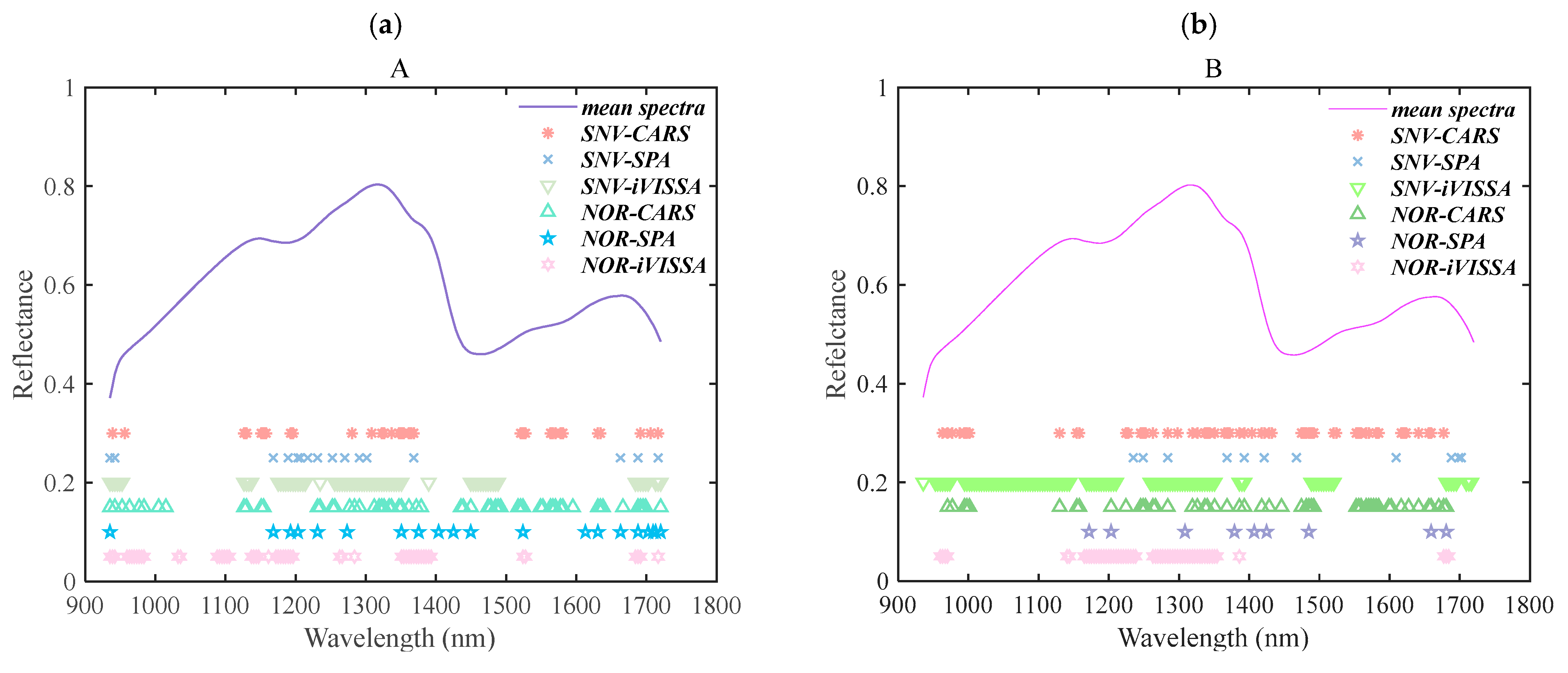
Figure 8 illustrates the distribution of characteristic bands for both side A and side B of the Exocarpium Citrus grandis, with feature extraction performed using two preprocessing methods: standard normal variate (SNV) and normalization (NOR). Despite employing different feature selection algorithms, several common spectral bands were observed across both sides, indicating inherent consistency in chemical composition. Under SNV preprocessing, the bands selected by the CARS algorithm exhibited similar distributions on side A and side B, suggesting that this method tended to identify stable spectral intervals regardless of spatial orientation. In contrast, the SPA algorithm demonstrated broader spectral coverage on side A—mainly within the 1100–1300 nm and 1500–1700 nm ranges—while on side B, its selections were more concentrated within 1300–1500 nm. This may reflect the SPA method’s sensitivity to side-dependent variations in spectral correlation structures. When applying NOR preprocessing, a similar trend was observed. CARS continued to select consistent bands across both sides, especially concentrated in the 1300–1500 nm and 1600–1700 nm regions, which corresponded to known absorption features of O–H and C–H functional groups, commonly associated with water and volatile metabolites. Meanwhile, SPA again showed wider selection on side A and narrower selection on side B, indicating its data-dependent selection bias.

Notably, the iVISSA algorithm showed strong cross-side consistency under both SNV and NOR, with its selected bands primarily located in the 1300–1500 nm and 1600–1700 nm ranges. These bands are associated with the vibrational overtones of moisture, sugars, and volatile organic compounds [31], suggesting that iVISSA—due to its adaptive and global search capability—can robustly capture chemically meaningful features less influenced by spatial side variations. This highlights iVISSA’s superior generalizability and stability compared to deterministic algorithms such as CARS and SPA.

Table 4. Model performance of CARS, SPA, and iVISSA feature spectral wavelengths for side A.

Model	Feature Extraction	Number of Bands	Accuracy (%)	Precision (%)	Recall (%)	F1-Score (%)
PLS-DA	CARS	33	85.13	86.61	85.19	84.17
	SPA	16	90.54	92.12	90.52	90.23
	iVISSA	73	86.49	87.77	86.50	85.77
RF	CARS	33	88.51	90.03	88.53	88.26
	SPA	16	83.11	83.79	83.18	83.14
	iVISSA	73	88.51	89.07	88.57	88.33
CNN	CARS	33	81.17 ± 2.49	86.86	83.78	82.80
	SPA	16	88.78 ± 1.55	90.81	90.61	90.55
	iVISSA	73	91.35 ± 0.56	92.26	91.91	91.98
BLS	CARS	58	91.08 ± 0.88	92.86	91.89	91.77
	SPA	20	92.97 ± 1.56	95.05	94.61	94.62
	iVISSA	54	94.09 ± 1.01	95.90	95.25	95.27

and

Table 5. Model performance of CARS, SPA, and iVISSA feature spectral wavelengths for side B.

Model	Feature Extraction	Number of Bands	Accuracy (%)	Precision (%)	Recall (%)	F1-Score (%)
PLS-DA	CARS	56	89.19	90.68	89.17	88.79
	SPA	11	86.49	88.64	86.47	85.94
	iVISSA	113	92.57	93.21	92.59	92.50
RF	CARS	56	83.48	84.33	83.85	83.66
	SPA	11	83.11	83.76	83.10	83.15
	iVISSA	113	92.57	93.44	92.57	92.39
CNN	CARS	56	87.97 ± 0.88	88.56	88.60	88.54
	SPA	11	89.19 ± 0.95	90.89	89.83	89.89
	iVISSA	113	87.57 ± 0.90	90.24	88.49	88.17
BLS	CARS	51	91.35 ± 1.11	93.46	93.30	93.30
	SPA	9	90.81 ± 0.77	92.22	91.95	91.96
	iVISSA	59	95.10 ± 0.82	96.34	95.95	95.97

exhibit the number of feature bands for different feature extraction methods. The differences in the number of bands selected by these methods were due to their inherent feature selection strategies. CARS tended to focus on the most relevant bands to the target variable (e.g., sample age), which led to fewer selected bands. SPA, on the other hand, selected fewer bands as it focused on the most important spectral features that maximized the projection effect, which reduced redundancy. iVISSA’s iterative and adaptive selection process allowed it to capture more bands, as it evaluated the contribution of each band to classification performance. While unifying the number of bands across methods might seem appealing for a fair comparison, it could potentially undercut the strengths of each method. Each algorithm is designed to operate most effectively with its optimal selection of bands, and forcing them to select the same number may lead to suboptimal results. Therefore, we allowed each method to select the optimal number of bands to best reflect its inherent advantages and achieve the highest classification performance.

3.5.2. Feature Wavelength Modeling

Table 4 and Table 5 summarize the modeling performance for side A and side B using three feature selection methods—CARS, SPA, and iVISSA—under their respective optimal preprocessing conditions. The results reveal that the impact of feature selection varied across different models, with the model structure and data characteristics playing a key role in performance differences. For PLS-DA, accuracy consistently improved with feature selection. For side A, SPA enhanced accuracy by 1.35%, while, for side B, iVISSA yielded a 2.71% increase. These improvements indicate that linear models like PLS-DA benefit from reduced dimensionality and the retention of highly linearly correlated bands, particularly effective for flavonoids and volatile-related wavelengths. For Random Forest (RF), the results were mixed. For side A, accuracy decreased after SPA selection, likely because SPA tends to extract a small number of strongly correlated features, which may reduce the diversity required for robust tree splitting. However, for side B, RF combined with iVISSA achieved a 3.38% improvement, suggesting that iVISSA preserved more complementary and discriminative bands, especially in regions associated with volatile compound absorption. In the case of the convolutional neural network (CNN), feature selection failed to enhance model performance on either side. This was attributed to the CNN’s reliance on learning hierarchical patterns directly from raw spectral inputs. When external feature selection is imposed, this disrupts the continuity and spatial correlations necessary for convolution operations, weakening the model’s ability to learn effective representations [32].

In contrast, the BLS consistently exhibited performance gains with selected features. For side A, the BLS + iVISSA model reached 95.27% accuracy, improving by 0.88% over the full-band input. For side B, accuracy further increased to 95.95%, representing a 2.03% gain. These results highlight the BLS’s suitability for working with compact, informative feature sets. The synergy between iVISSA’s adaptive band selection and the BLS’s dual-layer structure—comprising mapping and enhancement nodes—enables efficient learning while avoiding the complexity of deep architectures.

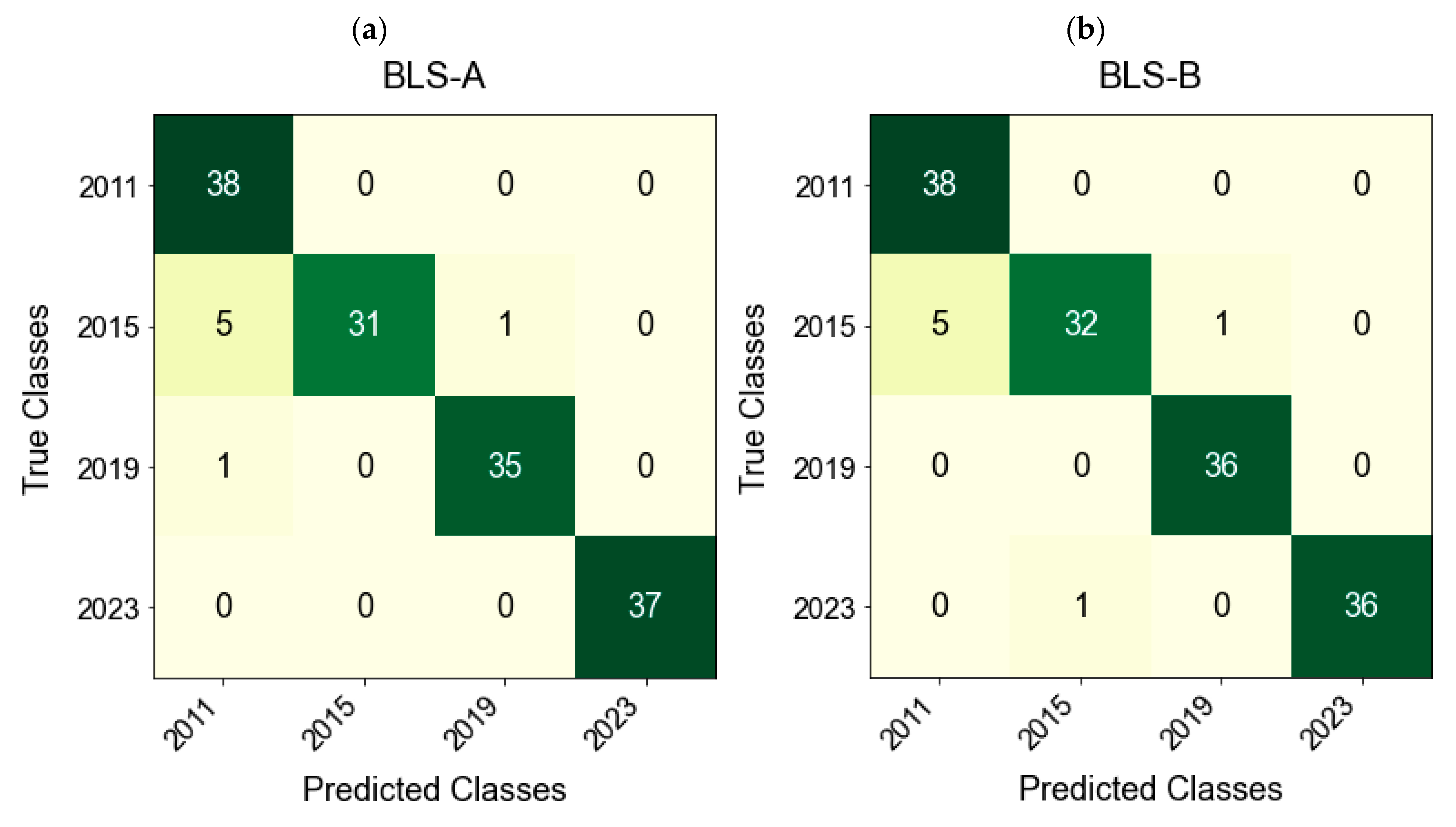
The confusion matrix in Figure 9 shows that the model reduced the misclassification of samples from 2011 and 2015, and the classification accuracy was improved. Specifically, the precision, recall, and F1-score were 95.90%, 95.25%, and 95.27% for side A and 96.34%, 95.95%, and 95.97% for side B, respectively. This result verifies the synergistic advantage between the feature extraction method and the model structure: iVISSA effectively screened key spectral information and provided highly relevant input features for the BLS, while the width expansion mechanism of the BLS enhanced the robustness of the model to the spectral differences between years while avoiding the limitation of the complexity of deep network training. Notably, the confusion matrix revealed residual misclassification between the 2011 and 2015 samples, despite their distinct average spectral profiles. This may have stemmed from intra-class variability, with some 2011 samples exhibiting higher reflectance and overlapping spectral features with early-stage 2015 samples. Moreover, the transition from early to mid-aging stages involved nonlinear and gradual chemical transformations, making the model more susceptible to boundary ambiguity during classification.

The comparison between side A and side B shows that the effect of the feature extraction method was closely related to the spectral distribution characteristics of the data. CARS tended to select features concentrated in the medium and short-wave bands for side A while expanding to a wider band range for side B, reflecting its adaptability under the differences in the spatial distribution of volatile substances in the samples. The feature selection of SPA covered a wider range for side A, while it was more concentrated on the feature interval related to flavonoids for side B, showing the difference in sensitivity of its screening strategy, which relied on the correlation between features of data for different sides. In contrast, iVISSA, with the help of the swarm intelligence optimization strategy, could dynamically identify band features that were highly correlated with target components (such as flavonoids and volatile substances), reducing its dependence on specific band distribution structures, and showed strong stability and adaptability for both side A and side B [33,34].

3.6. Mutual Verification of Both Sides

During hyperspectral image acquisition, it is often assumed that one side of the scanned sample is representative of the variation in the sample. However, this assumption may result in a calibration model that fails to predict the characteristics of the other side. In order to improve the adaptability of the model, using representative samples to cover the variation of different sides may be an effective solution. Therefore, it becomes particularly important to assess the impact of sampled sides on the vintage identification of Exocarpium Citri Grandis. When using spectral information from each side for classification, the models performed differently, but the overall differences were not significant. Therefore, we used side A and side B as training and test sets for alternate validation to further assess the stability and generalization ability of the models.

Table 6. Cross-validation results of BLS model between side A and side B using selected spectral features.

Training Data	Testing Data	Train Accuracy (%)	Test
			Accuracy (%)	Precision (%)	Recall (%)	F1-Score (%)
A	B	96.15	94.92	94.98	94.96	94.96
B	A	95.74	94.11	94.11	94.13	94.09

shows the results of the mutual validation of side A and side B, using NOR-iVISSA-BLS as the validation model. The results show that when side A was used as the training set and side B was used as the test set, the accuracy, precision, recall, and F1-score of the model were 94.92%, 94.98%, 94.96%, and 94.96%, respectively; when side B was used as the training set and side A was used as the test set, the accuracy, precision, recall, and F1-score were 94.11%, 94.11%, 94.13%, and 94.09%. All these results indicate that the model performed well and that the difference was not significant compared to the one-sided modeling results. Therefore, the effect of sampling side on the vintage identification of Exocarpium Citri grandis is negligible in practical applications.

4. Conclusions

In this study, hyperspectral imaging technology was applied to identify the aging year of Exocarpium Citri grandis by integrating different preprocessing methods, feature selection algorithms, and BLS. The proposed NOR–iVISSA–BLS achieved the best classification performance, with accuracy rates of 94.09 ± 1.01% and 95.10 ± 0.82% for side A and side B, respectively. Cross-side validation further demonstrated the robustness and generalizability of the model under small-sample conditions, with accuracy rates of 94.92% and 94.11%. These results indicate that the combination of dual-side spectral acquisition and lightweight learning models can effectively address intra-sample variability. However, this study was limited to a single variety from a single production region and did not evaluate adaptability to other citrus types, geographical sources, or broader field conditions. Future studies will focus on expanding the sample diversity to include multiple varieties and locations and assessing the practical implementation efficiency in industrial detection scenarios.

In terms of economic feasibility, although the initial setup cost for hyperspectral imaging (HSI) systems can be relatively high, they provide significant long-term benefits. By enabling non-destructive, high-throughput analysis, HSI reduces the need for extensive sample preparation and costly consumables, which can be particularly beneficial in industrial-scale applications. The ability to acquire large volumes of spectral data in a short period improves productivity and quality control, reducing operational costs over time. Therefore, integrating HSI into industrial production, especially in quality control and traceability for medicinal herbs, can be a cost-effective solution with a high return on investment. Overall, this study provides a promising and efficient approach for the vintage discrimination of Exocarpium Citri grandis, with the potential to support improved quality control and traceability in medicinal herb supply chains.