Article

Recovery of Optical Transport Coefficients Using Diffusion Approximation in Bilayered Tissues: A Theoretical Analysis

by
Suraj Rajasekhar
1 and
Karthik Vishwanath
1,2,*
1
Cellular, Molecular and Structural Biology Program, Miami University, 501 E High Street, Oxford, OH 45056, USA
2
Department of Physics, Miami University, 500 E Spring Street, Oxford, OH 45056, USA
*
Author to whom correspondence should be addressed.
Photonics 2025, 12(7), 698; https://doi.org/10.3390/photonics12070698
Submission received: 21 May 2025 / Revised: 6 July 2025 / Accepted: 8 July 2025 / Published: 10 July 2025
(This article belongs to the Special Issue Optical Technologies for Biomedical Science)

Abstract

Time-domain (TD) diffuse reflectance can be modeled using diffusion theory (DT) to non-invasively estimate optical transport coefficients of biological media, which serve as markers of tissue physiology. We employ an optimized N-layer DT solver in cylindrical geometry to reconstruct optical coefficients of bilayered media from TD reflectance generated via Monte Carlo (MC) simulations. Optical properties for 384 bilayered tissue models representing human head or limb tissues were obtained from the literature at three near-infrared wavelengths. MC data were fit using the layered DT model to simultaneously recover transport coefficients in both layers. Bottom-layer absorption was recovered with errors under 0.02 cm−1, and top-layer scattering was retrieved within 3 cm−1 of input values. In contrast, recovered bottom-layer scattering had mean errors exceeding 50%. Total hemoglobin concentration and oxygen saturation were reconstructed for the bottom layer to within 10 μM and 5%, respectively. Extracted transport coefficients were significantly more accurate when obtained using layered DT compared to the conventional, semi-infinite DT model. Our results suggest using improved theoretical modeling to analyze TD reflectance analysis significantly improves recovery of deep-layer absorption.

1. Introduction

Time-domain diffuse optical spectroscopy (TD-DOS) is a quantitative, non-invasive technique that has been widely explored across several biomedical applications [1,2,3,4,5]. The quantitative nature of this technique relies on recovering the wavelength-dependent transport coefficients—the absorption coefficient μ a ( λ ) and the reduced scattering μ s ( λ ) to optically characterize the medium from which measurements are obtained. While conventional DOS methods face broader optical hurdles such as speckle noise, often addressed via complex setups like ballistic imaging or T-matrix methods [6,7], TD-DOS overcomes these by leveraging photon time-of-flight to disentangle layered optical properties.
In TD-DOS, the measured temporal attenuation and broadening of an input source (which experimentally is usually a laser having pulse durations of 10–100 ps) is mathematically modeled using theoretical or numerical methods to recover the optical coefficients μ a ( λ ) and μ s ( λ ) [8,9,10,11,12]. In human tissues, accurate recovery of μ a ( λ ) at multiple wavelengths allows for reconstructions of component chromophore concentrations such as hemoglobin, water, and/or lipids, while μ s ( λ ) is influenced by tissue microstructure [8,11,13,14,15,16]. These chromophore concentrations are used to estimate tissue vascular oxygen saturation, total blood volume, hydration, and/or cellular density in vivo [17,18,19].
Theoretical models are critical for recovering optical transport coefficients from measurements, as they provide the quantitative platforms to model light transport in turbid media. A commonly used theoretical approach to quantify TD-DOS measurements is diffusion theory (DT) [20,21,22,23,24]. DT-based approaches typically consider the tissue medium as optically-homogeneous and semi-infinite in extent across various applications, including tracking and monitoring cerebral oxygenation and cancer development in clinical settings [3,10,21,25,26]. Though modeling biological tissues as a semi-infinite homogeneous medium allows for quantitative analysis, it is inherently insensitive to any inhomogeneities of the medium, which has been shown to lead to large errors in recovering physiological parameters [8,9,11,27,28,29].
Representing tissue as a bilayered medium would be more realistic than as a semi-infinite medium—e.g., a human head can be better modeled as having a top layer (representing scalp and skull) and a bottom layer (for the cerebral spinal fluid, gray and white matter), and limb tissues can be modeled as a layer of muscle buried under a upper layer of fat and skin [8,30]. The use of layered models in DT would permit reconstruction of optical coefficients for each layer, independently, from the measured TD reflectance [13,19,31]. Bilayered models can thus naturally detect transport coefficients of deeper layers better and can also be used to suppress cross-talk from superficial layers [2,23,32]. Such depth-dependent reconstructions would enhance the accuracy of cerebral and muscular hemodynamic assessments [2,31,32,33,34,35].
Analytical solutions of TD reflectance using DT in bilayered media have been reported previously [20,36,37,38,39]. However, they are not commonly used as the implementations face severe computational and numerical challenges due to their reliance on complex expressions involving hyperbolic functions and inverse integral transforms [29]. For layered media, nested integrations (e.g., inverse Hankel/Laplace transforms) exacerbate computational costs, with reported times of 0.5–5 s per solution—prohibitive for real-time applications [40]. Thus, these solvers have high computational complexity and costs [9,35,41,42,43,44]. LightPropagation.jl is a recently developed open source numerical solver that is stable and highly optimized (with a single calculation for a forward solution taking less than 0.5 ms on standard laptop computers) for computing time domain reflectance in multilayered tissue models via DT [29,45].
This work aims to assess both the accuracy and reliability of LightPropagation.jl in recovering known optical transport coefficients, thereby establishing its potential as a forward-inverse solver framework for reflectance signals from layered media. We utilize simulated reflectance signals generated via Monte Carlo simulations of time-resolved reflectance in bilayered tissue models. To ensure appropriate relevance to biomedical applications, we selected optical properties for tissue models simulated to match values reported in literature [30]. We use wavelength-dependent reconstructions to derive functional biological markers of oxygen saturation ( SO 2 ) and hemoglobin concentrations for each tissue layer and quantify the errors associated with reconstructions to establish limits for accuracy and precision of recovered optical coefficients and functional endpoints.

2. Materials and Methods

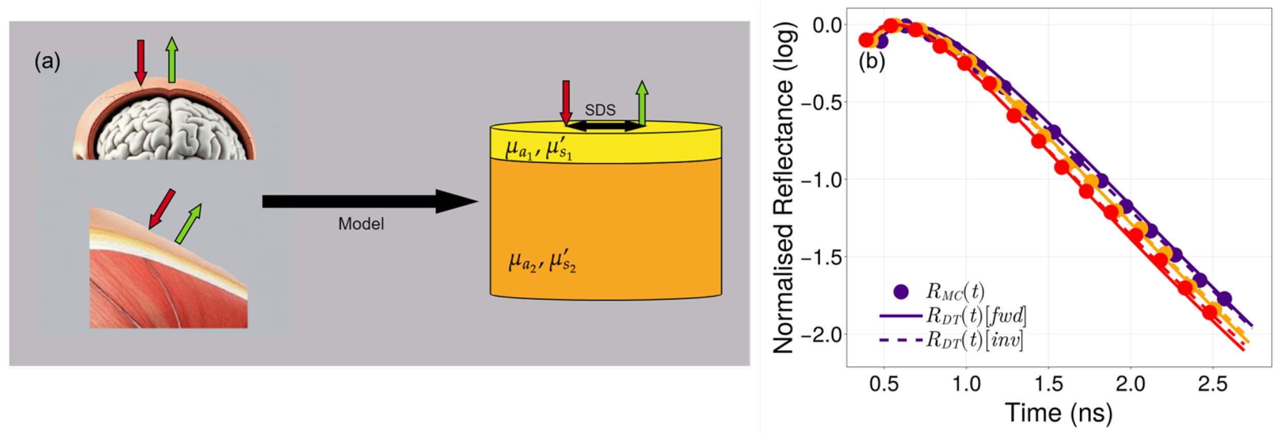
2.1. Bi-Layered Tissue Models

Two types of tissue models, representing head and limb muscle tissue were used to generate TD reflectance using MC simulations and are depicted by Figure 1a. Both tissue models were represented as cylinders with an upper layer thickness of 1 cm, and a semi-infinite bottom layer to compute MC and DT solutions. Input values of the absorption coefficient for each layer in each tissue model were determined solely by the percent oxygenation ( SO 2 ) and the total hemoglobin concentration ( [ T H b ] ). The total hemoglobin concentration is the sum of the oxygenated ( [ H b O ] ) and deoxygenated hemoglobin ( [ d H b ] ) concentrations, and SO 2 = 100 × [ H b O ] / [ T H b ] [46]. Table 1 lists values for inputs used to generate optical coefficients in each layer, for each tissue model.
Equation (1) determines the absorption coefficient μ a ( λ ) as a contribution from the two chromophores [ H b O ] and [ d H b ] . ϵ ( λ ) are extinction coefficients as a function of wavelength for each chromophore (subscripts). μ a for each layer was determined by using [ T H b ] and SO 2 values specified for each layer by the tissue model, while molar extinction coefficients were obtained from the literature [30,47]. The reduced scattering coefficients ( μ s ) for the top and bottom layer were calculated using Equation (2), which is a power-law approximating Mie scattering [30,48]. The exponent b and A are normalized following convention at 500 nm and values for these were obtained for each tissue type and layer from the literature [14,30].
μ a ( λ ) = [ T H b ] · ϵ H b O ( λ ) · SO 2 + ϵ d H b ( λ ) · ( 1 SO 2 )
μ s ( λ ) = A λ 500 b
A total of 64 different tissue models were generated at each of three commonly used near-infrared wavelengths (690, 760, and 850 nm) to span the isosbestic points of hemoglobin [8,16,22]. The full dataset for analysis consisted of 384   ( 64 × 3 × 2 ) bilayered tissue models. The average reduced albedo (defined as μ s / ( μ s + μ a ) ) was 0.98 ± 0.01 across both layers and all tissue models. Ranges for optical coefficients at each of the three wavelengths used, for each layer, are listed in Table A1, Table A2, and Table A3 for 690 nm, 760 nm, and 850 nm, respectively.

2.2. Monte Carlo Simulation of Reflectance Signals

A previously used Monte Carlo code for photon transport was used to simulate time-resolved reflectance from each of the 384 tissue models [49,50]. The MC model assumes the medium radius is infinite, and we set the bottom layer thickness to 100 cm to simulate a semi-infinite medium [51]. The top-layer thickness was set at 1 cm to best approximate the thicknesses of skull and adipose tissues [52,53]. MC simulations for all models were computed with 3 × 10 8 photon trajectories which was chosen from our preliminary analysis for a good signal-to-noise ratio (SNR) and falls in the range of photons generally used in MC simulations for diffuse optics [54,55]. For each simulation, the input source was a pencil beam (representing a delta-function) incident at the origin of the tissue model, and the TD diffuse reflectance was recorded between 1 cm and 3 cm in intervals of 0.25 cm with timing relative to the input delta-function source. Reflectance data was stored between 0 and 7 ns, with temporal resolution of 0.01 ns simulations run on a high-performance computing cluster (with each node of the cluster hosting Intel Xeon Gold processors (manufactured by Intel corporation, Santa Clara, CA, USA). Each MC simulation required about 15 h to execute, and simulations were run in parallel (on separate compute nodes) to increase output efficiency.
For analysis, each simulated time-resolved reflectance was smoothed (using a moving-window of span 5 or a temporal window of 0.05 ns), normalized (peak intensity was set to unity), truncated (retaining values greater than 80 % of peak intensity of the rising edge to eliminate early arriving photons, and discarding values lower than 0.001 % of the tail (to limit statistical noise)), and finally log-transformed, to obtain R M C ( t ) .

2.3. Forward-Modeling of Diffuse Reflectance Signal

The numerical DT solver (lightPropagation.jl) was used to compute TD-reflectance (as the temporal point spread function for an input delta-function source), in a bilayered cylindrical tissue model [29]. The SDS and layer thickness were set to match MC simulations and the refractive index of each layer was fixed at 1.4 following previous reports [56,57,58,59]. The top- and bottom-layer thickness were set to 1 cm and 100 cm, respectively, and matched MC simulations. The cylinder radius was also set to 100 cm. The large values for the radius and thickness ensured boundary reflections would not be collected [48,60]. Thus, computing any reflectance signal for a tissue model required inputs of its transport coefficients, μ a 1 , μ a 2 , μ s 1 , and μ s 2 . The computed reflectance was then truncated, normalized, and log-transformed following the same protocol used for processing the MC reflectance signal, to obtain R D T ( t ) .
Figure 1b shows representative data for TD-reflectance simulated (in symbols) and predicted from DT (solid lines) at three different wavelengths (colors) for a muscle tissue model. The values of optical absorption and scattering were calculated at each wavelength using Equations (1) and (2), where [ T H b ] was 18   μ M for the top layer and 27   μ M for the bottom layer, with both layers having SO 2 of 50%.

2.4. Inverse Fitting of Reflectance

Inverse modeling sought to recover the four optical transport coefficients (the absorption and scattering for each layer) by fitting each time-resolved reflectance R M C ( t ) , at each SDS, across each of the 384 tissue models. Fits were obtained iteratively using a Levenberg–Marquardt (LVM) non-linear optimizer (LsqFit package in Julia version 1.9.1) to compute a set of inputs to compute R D T ( t ) that best matched the input R M C ( t ) . For DT calculations, the top-layer thickness was assumed to be known (kept fixed for all analysis here at 1 cm), the refractive indices of both layers were held fixed at 1.4 and the SDS was set to match R M C ( t ) . The optimization by the LsqFit package was constrained with by keeping coefficients bounded between 0.01 < μ a < 0.5 for absorption and between 2 < μ s < 30 for scattering. This ensured that the inverse fits would only constrain the optical coefficients to specified ranges, to fit input data.
A normalized mean absolute error ( ζ ) value was computed to evaluate goodness of fits between R D T ( t ) and R M C ( t ) using Equation (3)
ζ = 1 N i = 1 N | R M C ( t i ) R D T ( t i ) | 1 N i = 1 N | R M C ( t i ) |
Here, R M C ( t i ) and R D T ( t i ) represent the reflectance signals from Monte Carlo simulations and the diffusion theory model, respectively, at time points t i . N represents the total number of time bins in R M C ( t i ) and N 180 ± 100 across the entire data-set, due to data truncation of R M C ( t ) as noted above.
For each simulated reflectance R M C ( t ) , inverse fitting was repeated until ζ was lower than 0.03 . If ζ was higher than the threshold after 25 attempts, the fit with lowest ζ was used to obtain optical coefficients. In Figure 1b, inverse fits are shown by dashed lines and had ζ of 0.017 ,   0.015   &   0.018 for the data shown at 690 nm (indigo), 760 nm (orange), and 850 nm (red), respectively.
Lastly, we also used the semi-infinite DT approximation to fit R M C ( t ) using lightPropagation.jl [45]. The forward fitting used in lightPropagation.jl replicates the expression for semi-infinite DT reflectance in Kienle et al. (1997) [37]. Inverse fitting for the semi-infinite model mirrored the bilayered approach, and used the optimizer algorithm to extract two coefficients μ a and μ s to the same goodness-of-fit threshold as used in the bi-layer reconstructions ( ζ = 0.03 ) and used the same search ranges for each optical coefficient ( 0.01 < μ a < 0.05 ; 2 < μ s < 30 ).

2.5. Retrieval of Functional Endpoints
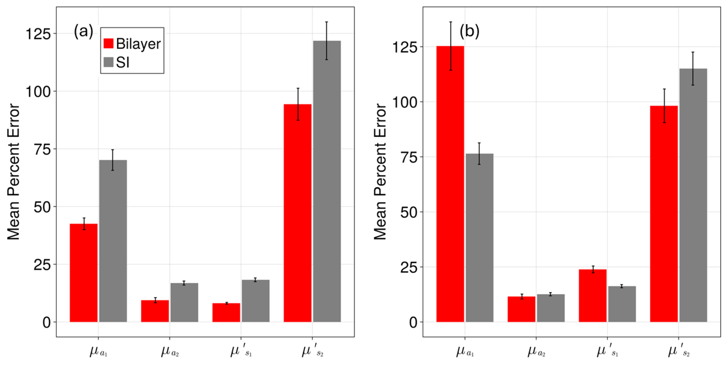
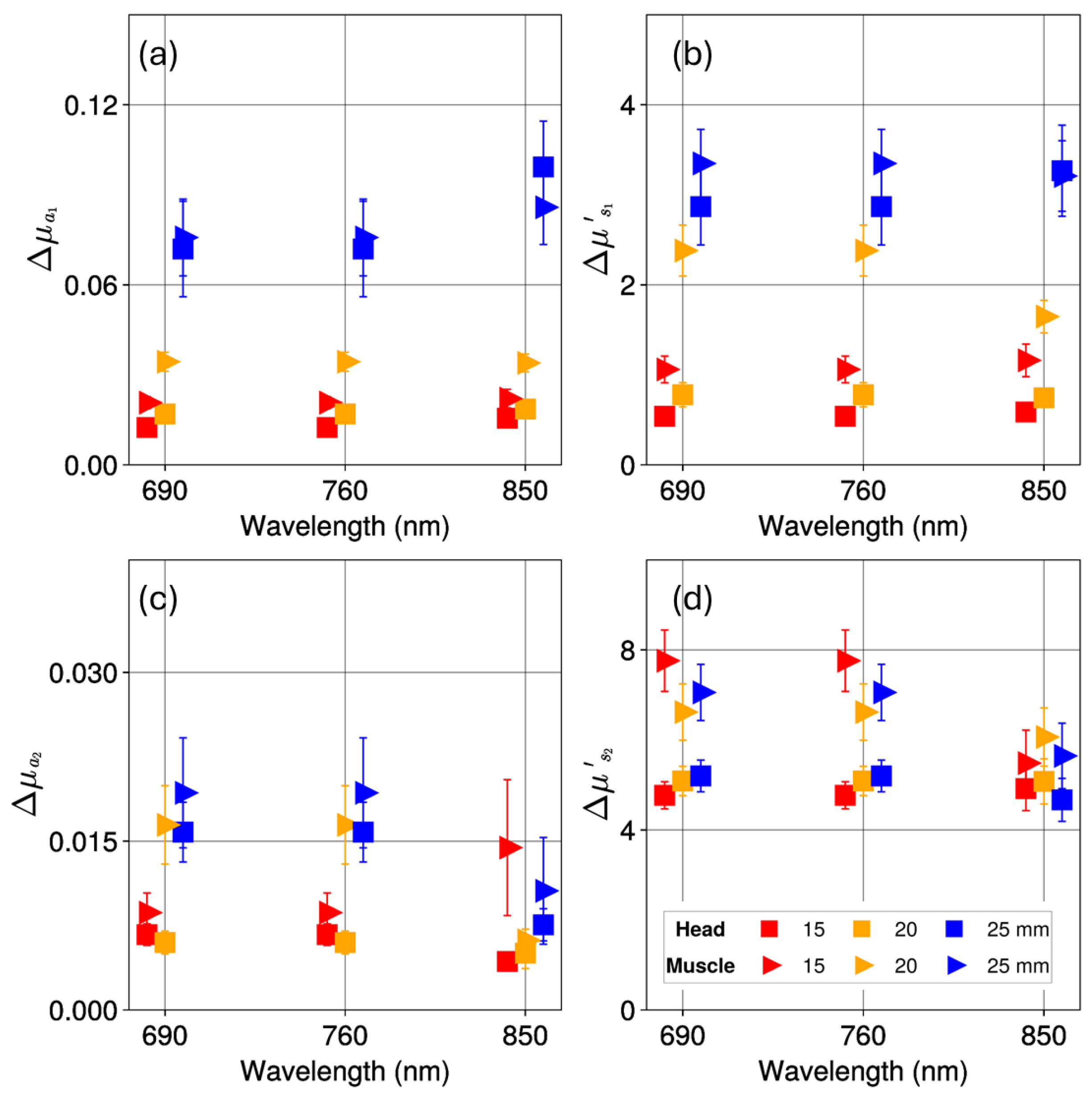
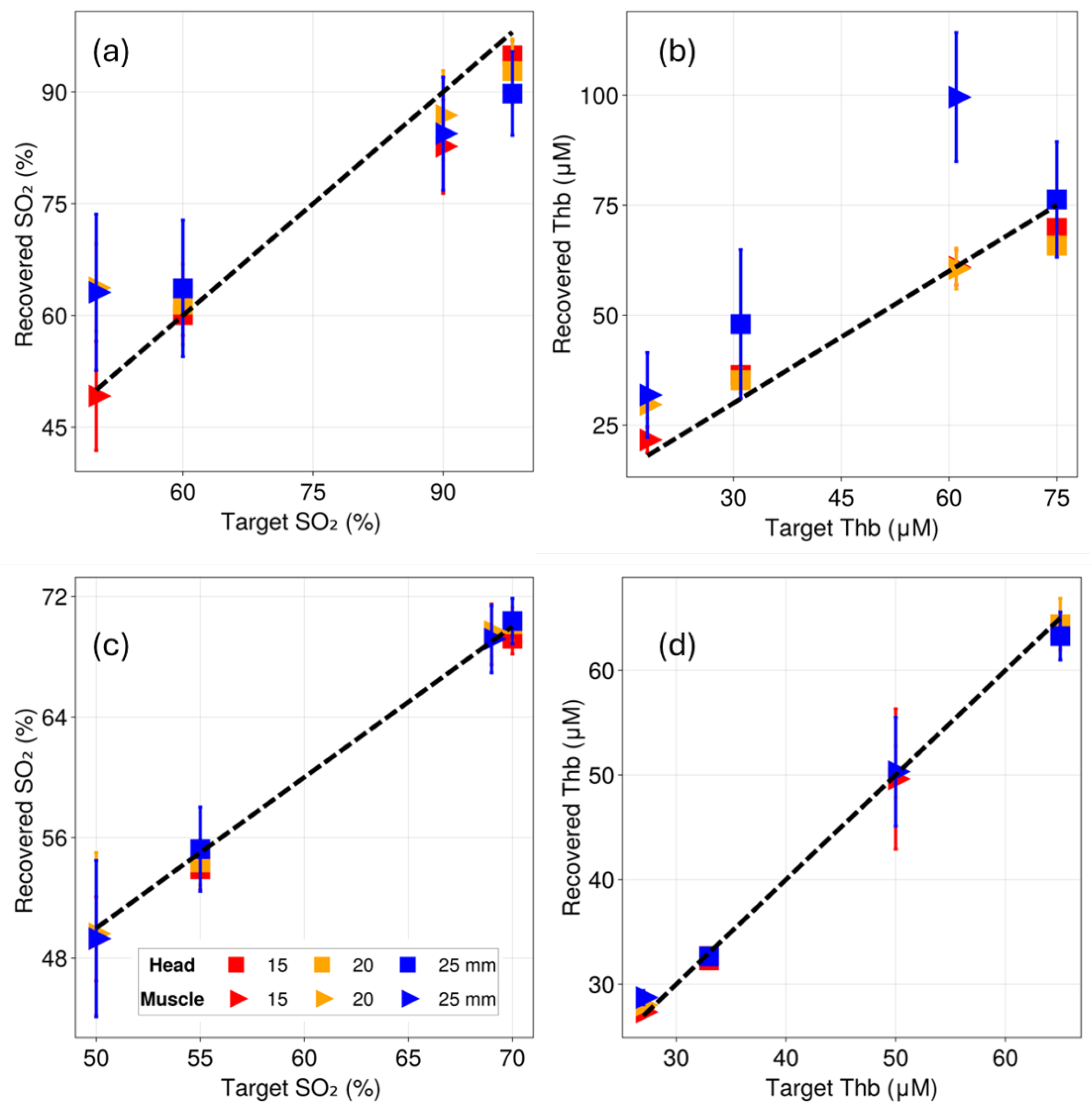
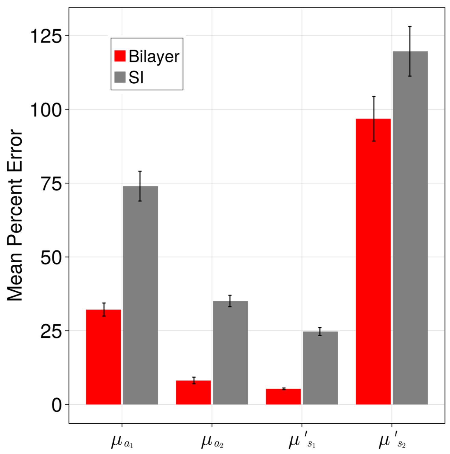
As most real-world applications of TD-DOS involve extracting tissue physiological parameters from optical coefficients, we emulated that process to the reconstructed absorption coefficients at multiple wavelengths to obtain the functional parameters of [ d H b ] and [ H b O ] using Equation (4)
μ a ( λ 1 ) μ a ( λ 2 ) μ a ( λ 3 ) = ϵ H b O ( λ 1 ) ϵ d H b ( λ 1 ) ϵ H b O ( λ 2 ) ϵ d H b ( λ 2 ) ϵ H b O ( λ 3 ) ϵ d H b ( λ 3 ) [ H b O ] [ d H b ]
Here, values of [ d H b ] and [ H b O ] were estimated using the same optimizer (as used for TD-reconstructions) to ensure only non-negative values of [ d H b ] and [ H b O ] were allowed as solutions by the optimizer. This eliminated any solutions with negative values for concentrations and thus remains physiologically meaningful. The chromophore concentrations were used to compute [ T H b ] (as [ d H b ] + [ H b O ] ) and SO 2 (as 100 × [ H b O ] / [ T H b ] ), which were each compared to input values used for the input tissue model (shown in Table 1). This process was repeated for each SDS.

3. Results

The inverse fitting protocol was employed to recover optical coefficients from each of the 384 MC models at three SDS. The average goodness of fits ζ at 1.5 cm and 2 cm were less than 0.01 across all model reconstructions. The head models fit better with an average ζ for head models equal to 0.007 , while the average ζ for muscle was 0.012 . At SDS of 2.5 cm, the average ζ increased to 0.02 , which could also be due to low photon statistics in MC simulations. A single inverse fit for each tissue model took approximately 10–15 s on average. However, inverse fits were iterated on average 10 times to satisfy the ζ threshold. Thus, the computation time for each tissue model (at each SDS) took nearly 150 s. Reconstructed errors in the absorption ( μ a 1 , μ a 2 ) and reduced scattering coefficients ( μ s 1 , μ s 2 ), across all simulated tissue models are shown in Figure 2.
Figure 2d shows that the largest errors were in recovery of bottom layer scattering μ s 2 often exceeding 5   cm 1 across all SDS. The difficulty of reconstructing deep-layer scattering with DT is well known as reported previously [20,61,62,63]. The mean absolute error in the recovery of μ a 1 (Figure 2a) was less than 0.03   cm 1 at SDS of 1.5 cm and 2 cm. Errors increased to nearly 0.1   cm 1 at SDS of 2.5 cm, which was as expected, as photon paths probe deeper layers at longer SDS. The recoveries of μ a 2 and μ s 1 were the most accurate and showed errors lower than 0.02   cm 1 and 3   cm 1 , respectively, at all SDS tested (Figure 2b,c). These data are visualized as recovered vs. target values in Figure A1, Figure A2 and Figure A3 for each of the three wavelengths used.
The impact of reconstruction errors on derived physiological parameters was next investigated by reconstructing concentrations of ( [ d H b ] ) and ( [ H b O ] ) and shown in Figure 3. These concentrations were recovered using the absorption coefficients obtained at 690 nm, 760 nm, and 850 nm using Equation (4). Note that the x-axes in all panels are scaled according to the actual hemoglobin concentrations used across all tissue models simulated. As a result, the spacing between adjacent bars is not uniform and shows an uneven distribution of values spanned by the tissue models used here.
The results in Figure 3a,b, demonstrate that top-layer hemoglobin retrieval was less accurate than reconstructions in the bottom layer. Most of the recovered values in the upper layer either overestimated the deoxygenated hemoglobin values (for smaller values of [ d H b ] ) or underestimated it (for larger values of [ d H b ] ). However, the error bars (standard error) were within 10   μ M across all models, presenting sufficient resolution for clinical use cases [64]. Reconstructions for bottom-layer concentrations were robust, with recovered values of both [ d H b ] and [ H b O ] being well within acceptable ranges of target values (Figure 3c,d).
Functionally, the optical biomarkers sought by real-world applications using TD-DOS are the total hemoglobin concentration [ T H b ] and percent oxygen saturation SO 2 . Figure 4 shows the input SO 2 and total hemoglobin concentration ( [ T H b ] ) values for the top and bottom layers, compared to the values recovered using the bilayered inverse DT. As anticipated, errors in hemoglobin concentrations in the top layer impact the accuracy of both physiological markers SO 2 and [ T H b ] , leading to significant deviations from their true values. The median reconstructed values differ from the expected values, and have higher error bars with larger SDS.
However, both precision and accuracy of SO 2 and [ T H b ] in the bottom layer (Figure 4c,d) was high. Reconstructed values matched target values to better than 3% across all SDS. There was one notable exception for muscle models that had [ T H b ] = 50   μ M and SO 2 = 50 % for the bottom layer—these models exhibited a large variance in reconstructed values (the median was still within 3% of the target value).
To conclude our analysis, we reconstructed optical coefficients from the TD reflectance simulated by bilayered R M C ( t ) using the semi-infinite DT reflectance expression [37]. Since the SI model could only reconstruct one pair of optical coefficients ( μ a   and   μ s ), we compare the recovered absorption coefficient here to both μ a 1 and μ a 2 and likewise for scattering. Figure 5 shows the mean percent error (bars) along with the standard error (error bars) across all MC models used for reconstructions at 15 mm SDS. The data indicate that the layer-specific transport coefficients were always more accurate when reconstructed with layered DT than those estimated by the semi-infinite DT. The notable exception was for retrieval of μ s 2 where the two theoretical models were comparable to each other. These trends remained consistent at SDS = 2 cm, but at SDS = 2.5 cm, the reconstruction of μ a 1 seemed better when recovered from semi-infinite DT (Figure A6).

4. Discussion

We verified the performance of an open-source, numerical solver of DT in cylindrical coordinates for layered media, lightpropagation.jl, to function as an inverse solver in bilayer tissue models using TD reflectance simulated at multiple SDS. A total of 384 bilayered tissue models spanning a range of optical properties reported for head and muscle tissues were used to generate TD reflectance from MC simulations. For each model, a goodness of fit was established by computing the normalized mean absolute error ( ζ ), between the simulated reflectance and the DT fitted reflectance. The average ζ was lower than 0.01 at SDS of 1.5 and 2 cm and increased to 0.02 at SDS of 2.5 cm. A change of 0.01 in ζ in goodness of fit was significant and impacted accuracy of reconstructions of the top layer absorption μ a 1 as seen in Figure 2a. Thus, ζ could potentially signal a measure of confidence in the retrieved value of optical coefficients for each fitted reflectance and could also serve as a measure of signal quality in experimental use.
A threshold of ζ less than 0.02 in inverse fits of the reflectance was sufficient for reconstruction of top layer scattering ( μ s 1 ) and the bottom layer absorption ( μ a 2 ) with median errors of lesser than 5% for μ a 2 and lesser than 6% for μ s 1 ), across all SDS tested and as shown in Figure 2b,c (and Table 2). However, the scattering of the bottom layer ( μ s 2 ) could not be reconstructed accurately and showed a median error of more than 45% across all SDS (Table 2), indicating layered DT is largely unperturbed by changes in deep-layer scattering, as reported before [9,20,39,62,63]. Although recovery of top layer absorption μ a 1 was achieved, it was inconsistent, with median errors lesser than 20 % for all 384 models at SDS of 1.5 and 2 cm that increased to more than 50 % for SDS of 2.5 cm, which indicates that the reconstruction upper-layer absorption was sensitive to SNR. These trends in recovery as compared to the target values are shown in Figure A1, Figure A2 and Figure A3.
The input coefficients for each tissue model simulated here were obtained by assuming only two chromophores ( [ d H b ] and [ H b O ] ) were present in each layer. The values shown in Table 1 are the derived quantities SO 2 and [ T H b ] that were used as the input values to compute the transport coefficients. In the inverse sense, these chromophore concentrations had to be obtained from reconstructed absorption coefficients, for each layer, at each wavelength. Thus, as expected, errors in recovery of μ a 1 impacted the estimation of oxygenated and deoxygenated hemoglobin concentrations for the upper layer, with median error being higher than 5 ± 2   μ M but lower than 10 ± 3   μ M for SDS 1.5   and   2 cm (Figure 3a,b and Figure A4a,b). The upper bound on top-layer concentration errors grew to more than 15   μ M for both chromophore concentrations at SDS of 2.5 cm (Figure A5a,b). The bottom-layer reconstructions demonstrated good agreement with ground truth values (to better than 3   μ M at all SDS) while also having small standard errors.
Accurate recovery of individual chromophore concentrations is important, as clinically relevant parameters such as oxygen saturation ( SO 2 ) and total hemoglobin concentration ( [ T H b ] ) are derived from the combined contributions of [ H b O ] and [ d H b ] as markers of tissue health and metabolic demand. Errors in reconstruction of the top-layer chromophore concentrations thus impacted retrieval of top layer SO 2 (median error larger than 5% for all SDS). The top-layer [ T H b ] values were retrieved with median errors greater than 15% for shorter SDS (1.5 and 2 cm), which increased to more than 60 % for larger SDS (Figure 4a,b). Again, this is consistent with the idea that the diffuse reflectance collected at larger SDS would be most insensitive to upper layer optical coefficients.
These results highlight that bilayered DT has reduced sensitivity to the top layer absorption, and reconstruction of μ a 1 is sensitive to signal quality. However, recovery of bottom-layer endpoints was accurate with SO 2 and [ T H b ] being estimated to better than 4% across all SDS. This result is particularly encouraging, as it suggests that real-world applications could achieve improved quantitative sensitivity to functional properties in deeper tissue layers. This can be accomplished while remaining robust to changes in superficial layers by using more accurate analytical models for reconstructing time-domain reflectance [13,65,66].
A practical consideration that remained significant was the computational cost involved with reconstructions using the bilayer inverse model. The inverse fits converged in under 100 milliseconds using the analytical DT expression for an SI model, while for bilayer reconstructions, inverse fits were approximately three orders of magnitude slower (taking, on average, about 150 s for each model). All inverse calculations were run on nodes of a high-performance computing cluster (with each node having an Intel Xeon Gold processor). For the 384 models analyzed at 3 SDS, the total computation time was almost 40 CPU-hours. This disparity presents a significant bottleneck for real-time or high-throughput analysis and motivates the development of computationally efficient strategies or machine-learning based models for acceleration.
Ultimately, the computational costs were recovered by the layered model as it consistently outperformed the semi-infinite model in terms of accuracy to recover μ a 2 and μ s 1 even at large SDS (Figure 5 and Figure A6). On average, the bilayered modeling performed better than SI model, to extract optical absorption. For example, in a head tissue model that was simulated with top and bottom layer oxygenation of 98 % and 70 % , the error in recovered cerebral oxygenation was 2.7 % when reconstructed with bilayer DT at an SDS of 1.5 cm, but it was 13 % when reconstructed with semi-infinite DT. The error in retrieval of cerebral oxygenation is comparable between semi-infinite and bilayer models (within 1% of each other) for only 31 models of the 384 tested. In the case of a particular head tissue model that had top- and bottom-layer oxygen saturation of 60 % and 55 % , respectively, semi-infinite and bilayered models recovered cerebral oxygenation to within 1.5% at and SDS of 1.5 cm, the semi-infinite model marginally underperformed the bilayered estimate. It is interesting to note that bilayered DT models could extract μ a 2 accurately, even at short SDS (of 1 cm), which may prove to be practically useful, as shorter SDS channels have better SNR.
The mean and median global errors for all optical coefficients, as well as the functional endpoints, along with the standard deviations of the errors are listed in Table 2 to clearly compare the performance of extracting the coefficients from semi-infinite and bilayered DT.
Our exploration establishes the advantage of bilayer DT modeling by comparing the accuracy of the retrieval of optical coefficients and the functional endpoints across a large range of optical coefficients representing two standard target tissues. We also explicitly compare the performance of semi-infinite and bilayer DT models for the first time, to the best of our knowledge. The exploration, however, was limited to an a priori assumption of the top-layer thickness and a uniform refractive index for both layers. Further exploration on the effect that these physical parameters can have need to be explored.

5. Conclusions

We demonstrate that using multi-layer DT for analysis of TD reflectance simulated in bilayered media allowed for quantitative reconstruction of optical absorption of both layers. Accuracy and precision of recovered parameters were within acceptable ranges for clinical utility across a wide-set of target optical coefficients. The top-layer absorption coefficient ( μ a 1 ) was reconstructed with mean errors lesser than 0.03   cm 1 at SDS of 1.5   and   2 cm (rising to greater than 0.1   cm 1 at 2.5 cm), while the reduced scattering coefficient ( μ s 1 ) was recovered to within 3   cm 1 across all SDS. The average errors in bottom layer absorption, μ a 2 were within 0.02   cm 1 of their true values, while bottom layer scattering μ s 2 could had errors larger than 50%. When translated into errors in functional endpoints, the top-layer [ T H b ] and SO 2 had larger errors relative to the bottom layer. Our work also showed that the accuracy of retrieved optical coefficients and their corresponding functional endpoints using layered DT and over-performed the semi-infinite DT model across all retrieved optical coefficients. However, the layered DT had significantly higher computational costs. Future work will investigate approaches to reduce computational time for optimization of TD-reflectance.

Author Contributions

Conceptualization, S.R. and K.V.; methodology, S.R. and K.V.; software, S.R.; validation, S.R. and K.V.; investigation, S.R.; writing—original draft preparation, S.R.; writing—review and editing, S.R. and K.V.; visualization, S.R.; supervision, K.V. All authors have read and agreed to the published version of the manuscript.

Funding

This research received no external funding.

Institutional Review Board Statement

Not applicable.

Informed Consent Statement

Not applicable.

Data Availability Statement

LightPropagation.jl is a registered Julia package that can be installed on a Julia version > 1.5. The MC simulations and inverse fitting codes are available on request.

Acknowledgments

We thank Michael Helton, the developer of LightPropagation.jl, for their input in using the toolbox. We also thank Jens Müller for facilitating high-performance simulations on the Miami Redhawk cluster.

Conflicts of Interest

The authors declare no conflicts of interest.

Abbreviations

The following abbreviations are used in this manuscript:
SISemi Infinite
DTDiffusion Theory
MCMonte Carlo
dHbdeoxygenated hemoglobin
HbOoxygenated hemoglobin
THbTotal Hemoglobin Concentration
SO 2 Fractional Oxygen Saturation
SDSSource Detector Separation
SNRSignal-to-Noise Ratio
LVMLevenberg–Marquardt Method
TDTime Domain
DOSDiffuse Optical Spectroscopy

Appendix A. Computed Optical Transport Coefficients

Here we report the computed optical coefficients using the ranges for SO 2 and [ T H b ] described in Table 1.
Table A1. The selected target tissue properties. The values below were calculated for λ = 690 nm. The value reported for each optical property is the mean of the coefficients (4 for absorption for each layer and 2 for scattering for each layer) along with the range covering all the computed values. The coefficient values used for our analysis for each model, however, were not evenly spread within this range.
Tissue ModelLayer μ a   cm 1 μ s   cm 1
HeadTop (scalp, skull) 0.096 ± 0.074 13.329 ± 3.868
Bottom (Brain) 0.111 ± 0.050 14.81 ± 0.271
MuscleTop (skin, fat) 0.093 ± 0.041 18.854 ± 6.752
Bottom (Muscle) 0.088 ± 0.046 6.822 ± 2.844
Table A2. The values below were calculated for λ = 760 nm.
Tissue ModelLayer μ a   cm 1 μ s   cm 1
HeadTop (scalp, skull) 0.105 ± 0.062 12.823 ± 3.868
Bottom (Brain) 0.109 ± 0.043 12.068 ± 0.88
MuscleTop (skin, fat) 0.089 ± 0.061 17.467 ± 5.807
Bottom (Muscle) 0.089 ± 0.034 5.939 ± 2.905
Table A3. The values below were calculated for λ = 850 nm.
Tissue ModelLayer μ a   cm 1 μ s   cm 1
HeadTop (scalp, skull) 0.123 ± 0.058 12.267 ± 3.451
Bottom (Brain) 0.104 ± 0.038 9.619 ± 1.702
MuscleTop (skin, fat) 0.090 ± 0.0574 16.003 ± 4.835
Bottom (Muscle) 0.081 ± 0.028 5.098 ± 2.880

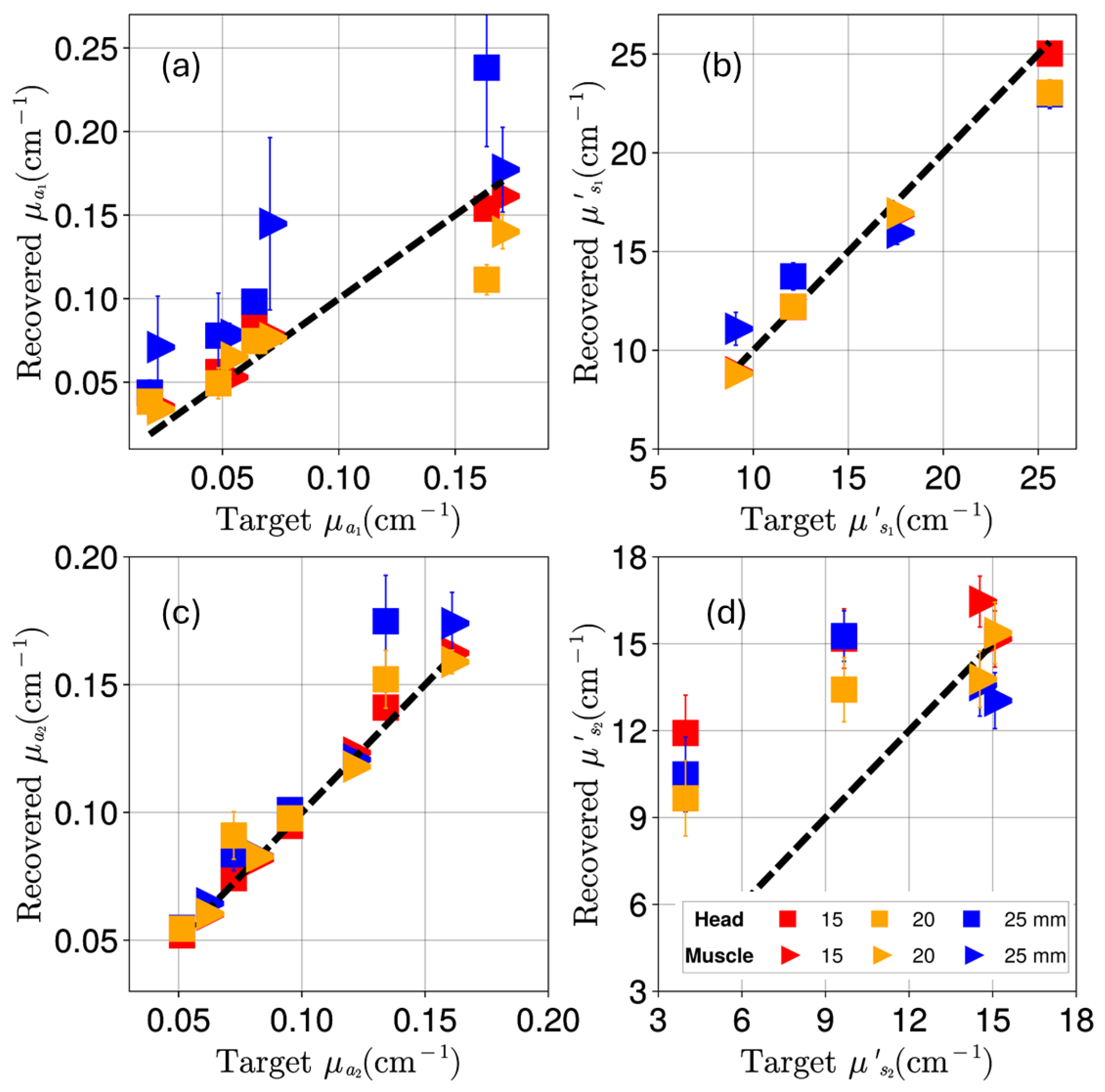
Appendix B. Reconstruction of Optical Coefficients

In Figure A1 each marker corresponds to some fixed value for the optical coefficient being plotted, while the other three coefficients were varied. For instance, each marker in Figure A1a is from 16 different tissue models that shared the same μ a 1 value, while error bars are the standard error across all those 16 reconstructed values of μ a 1 as μ a 2 , μ s 1 and μ s 2 were permuted. The Figure A2 and Figure A3 illustrate the reconstruction of the optical coefficients at wavelengths of 690 nm and 850 nm, respectively.
Figure A1. Target versus recovered optical coefficients at 760 nm for absorption ( μ a 1 and μ a 2 in (a,c) and reduced scattering coefficients ( μ s 1 , μ s 2 in (b,d)) across each of the 64 models for brain (squares) and the 64 models for muscle (triangles). Colors represent different SDS: red for 1.5 cm, orange for 2 cm and blue for 2.5 cm and the dashed black line represents the y = x line. The error bars represent the standard error across all models that share fixed values of each optical coefficient under investigation. It is important to note that there are six different markers each with its own error bar. Many of the error bars are smaller than the marker sizes used.
Photonics 12 00698 g0a1
Figure A2. Target vs. recovered μ a 1 , μ a 2 (a,c) and μ s 1 , μ s 2 (b,d) at 690 nm for brain (squares) and muscle (triangles). Colors indicate SDS (red: 1.5 cm, orange: 2 cm, blue: 2.5 cm). Dashed black line: y = x .
Photonics 12 00698 g0a2
Figure A3. Target vs. recovered μ a 1 , μ a 2 (a,c) and μ s 1 , μ s 2 (b,d) at 850 nm for brain (squares) and muscle (triangles). Colors indicate SDS (red: 1.5 cm, orange: 2 cm, blue: 2.5 cm). Dashed black line: y = x .
Photonics 12 00698 g0a3

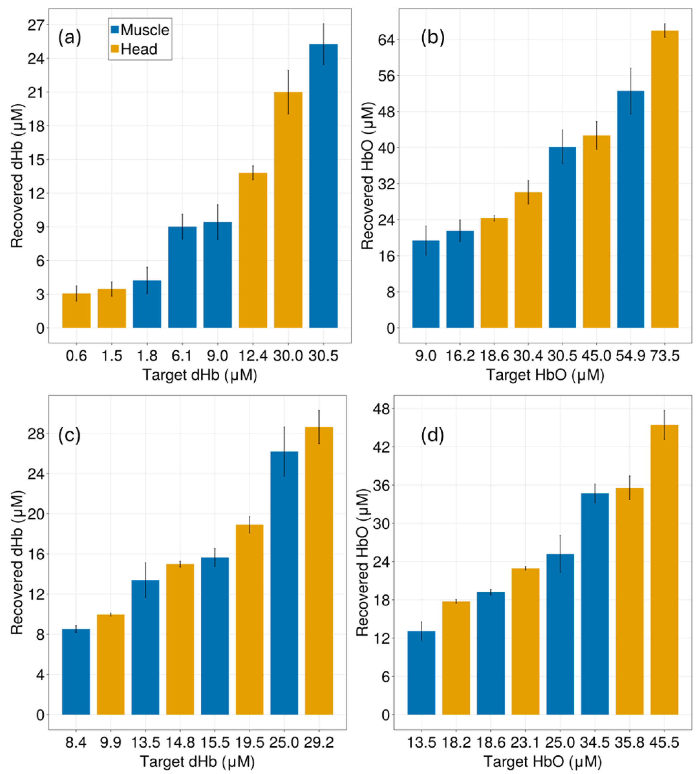
Appendix C. Reconstruction of Deoxygenated and Oxygenated Hemoglobin Concentrations

Figure A4. The reconstructed chromophore concentrations at 2 cm. Subplots (a,b) represent the top-layer and (c,d), the bottom-layer reconstruction of [ d H b ] and [ H b O ] , respectively. Here, similar to Figure 3, the x-axis is not evenly spaced to avoid sparsely populated graph.
Photonics 12 00698 g0a4
Figure A5. The reconstructed chromophore concentration at 2.5 cm. Subplots (a,b) represent the top-layer and (c,d), the bottom-layer reconstruction of [ d H b ] and [ H b O ] , respectively. Here, similar to Figure 3, the x-axis is not evenly spaced to avoid sparsely populated graph. Notably, top-layer estimates show greater error.
Photonics 12 00698 g0a5

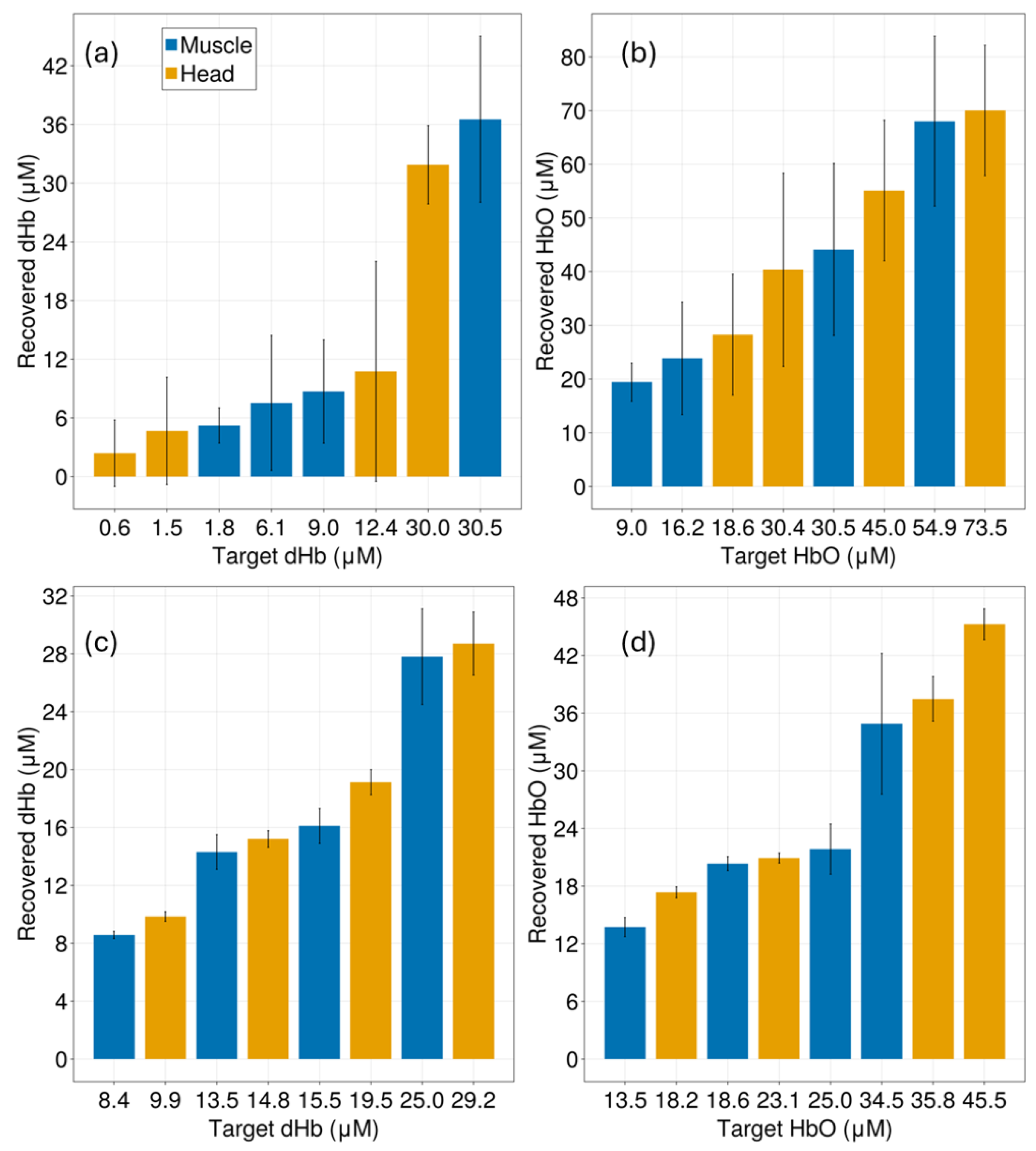
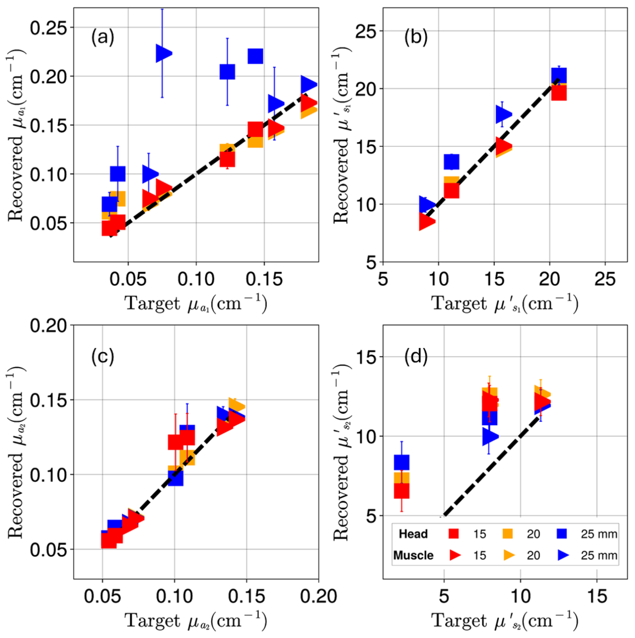
Appendix D. Reconstruction of Optical Coefficients Using Semi-Infinite Tissue Approximation

Figure A6. Comparison of percent errors in the reconstructed optical properties for the bilayered and semi-infinite (SI) models. The sub-figures (a,b), correspond to SDS = 2 and 2.5 cm respectively. The optical properties analyzed include the absorption coefficients of the first and second layers ( μ a 1 , μ a 2 ) and the reduced scattering coefficients of the first and second layers ( μ s 1 , μ s 2 ) labeled as groups along the x-axis.
Photonics 12 00698 g0a6

References

  1. Blaney, G.; Donaldson, R.; Mushtak, S.; Nguyen, H.; Vignale, L.; Fernandez, C.; Pham, T.; Sassaroli, A.; Fantini, S. Dual-Slope Diffuse Reflectance Instrument for Calibration-Free Broadband Spectroscopy. Appl. Sci. 2021, 11, 1757. [Google Scholar] [CrossRef] [PubMed]
  2. Shimada, M.; Hoshi, Y.; Yamada, Y. Simple algorithm for the measurement of absorption coefficients of a two-layered medium by spatially resolved and time-resolved reflectance. Appl. Opt. 2005, 44, 7554–7563. [Google Scholar] [CrossRef]
  3. Sekar, S.K.V.; Lanka, P.; Farina, A.; Mora, A.D.; Andersson-Engels, S.; Taroni, P.; Pifferi, A. Broadband Time Domain Diffuse Optical Reflectance Spectroscopy: A Review of Systems, Methods, and Applications. Appl. Sci. 2019, 9, 5465. [Google Scholar] [CrossRef]
  4. Ugai, T.; Sasamoto, N.; Lee, H.Y.; Ando, M.; Song, M.; Tamimi, R.M.; Kawachi, I.; Campbell, P.T.; Giovannucci, E.L.; Weiderpass, E.; et al. Is early-onset cancer an emerging global epidemic? Current evidence and future implications. Nat. Rev. Clin. Oncol. 2022, 19, 656–673. [Google Scholar] [CrossRef]
  5. Ferrari, M.; Quaresima, V. A brief review on the history of human functional near-infrared spectroscopy (fNIRS) development and fields of application. NeuroImage 2012, 63, 921–935. [Google Scholar] [CrossRef] [PubMed]
  6. Georgakoudi, I.; Rice, W.L.; Hronik-Tupaj, M. Optical spectroscopy and imaging for the noninvasive evaluation of engineered tissues. Tissue Eng. Part. Rev. 2008, 14, 321–340. [Google Scholar] [CrossRef]
  7. Conkey, D.B.; Brown, A.N.; Caravaca-Aguirre, A.M.; Piestun, R. Non-invasive focusing and imaging in scattering media with a fluorescence-based transmission matrix. Nat. Commun. 2020, 11, 6154. [Google Scholar] [CrossRef]
  8. Yamada, Y.; Suzuki, H.; Yamashita, Y. Time-Domain Near-Infrared Spectroscopy and Imaging: A Review. Appl. Sci. 2019, 9, 1127. [Google Scholar] [CrossRef]
  9. Pifferi, A.; Contini, D.; Mora, A.D.; Farina, A.; Spinelli, L.; Torricelli, A. New frontiers in time-domain diffuse optics, a review. J. Biomed. Opt. 2016, 21, 091310. [Google Scholar] [CrossRef]
  10. Boer, L.L.D.; Bydlon, T.M.; Duijnhoven, F.V.; Peeters, M.J.T.V.; Loo, C.E.; Winter-Warnars, G.A.; Sanders, J.; Sterenborg, H.J.; Hendriks, B.H.; Ruers, T.J. Towards the use of diffuse reflectance spectroscopy for real-time in vivo detection of breast cancer during surgery. J. Transl. Med. 2018, 16, 367. [Google Scholar] [CrossRef]
  11. Hallacoglu, B. Absolute measurement of cerebral optical coefficients, hemoglobin concentration and oxygen saturation in old and young adults with near-infrared spectroscopy. J. Biomed. Opt. 2012, 17, 081406. [Google Scholar] [CrossRef] [PubMed]
  12. Farina, A.; Torricelli, A.; Bargigia, I.; Spinelli, L.; Cubeddu, R.; Foschum, F.; Jäger, M.; Simon, E.; Fugger, O.; Kienle, A.; et al. In-vivo multilaboratory investigation of the optical properties of the human head. Biomed. Opt. Express 2015, 6, 2609–2623. [Google Scholar] [CrossRef] [PubMed]
  13. Calcaterra, V.; Lacerenza, M.; Amendola, C.; Buttafava, M.; Contini, D.; Rossi, V.; Spinelli, L.; Zanelli, S.; Zuccotti, G.; Torricelli, A. Cerebral baseline optical and hemodynamic properties in pediatric population: A large cohort time-domain near-infrared spectroscopy study. Neurophotonics 2024, 11, 045009. [Google Scholar] [CrossRef]
  14. Bossi, A.; Bianchi, L.; Saccomandi, P.; Pifferi, A. Optical signatures of thermal damage on ex-vivo brain, lung and heart tissues using time-domain diffuse optical spectroscopy. Biomed. Opt. Express 2024, 15, 2481–2497. [Google Scholar] [CrossRef]
  15. Martelli, F.; Binzoni, T.; Bianco, S.D.; Liemert, A.; Kienle, A. Light Propagation Through Biological Tissue and Other Diffusive Media_ Theory, Solutions, and Validations; SPIE: Washington, DC, USA, 2022. [Google Scholar]
  16. Hoshi, Y. New Horizons in Time-Domain Diffuse Optical Spectroscopy and Imaging; MDPI: Basel, Switzerland, 2020. [Google Scholar]
  17. Blaney, G.; Sassaroli, A.; Fantini, S. Spatial sensitivity to absorption changes for various near-infrared spectroscopy methods: A compendium review. J. Innov. Opt. Health Sci. 2024, 17, 2430001. [Google Scholar] [CrossRef]
  18. Wada, H.; Yoshizawa, N.; Ohmae, E.; Ueda, Y.; Yoshimoto, K.; Mimura, T.; Nasu, H.; Asano, Y.; Ogura, H.; Sakahara, H.; et al. Water and lipid content of breast tissue measured by six-wavelength time-domain diffuse optical spectroscopy. J. Biomed. Opt. 2022, 27, 105002. [Google Scholar] [CrossRef]
  19. Tagliabue, S.; Kacprzak, M.; Rey-Perez, A.; Baena, J.; Riveiro, M.; Maruccia, F.; Fischer, J.B.; Poca, M.A.; Durduran, T. How the heterogeneity of the severely injured brain affects hybrid diffuse optical signals: Case examples and guidelines. Neurophotonics 2024, 11, 045005. [Google Scholar] [CrossRef] [PubMed]
  20. Kienle, A.; Glanzmann, T.; Wagnières, G.; van den Bergh, H. Investigation of two-layered turbid media with time-resolved reflectance. Appl. Opt. 1998, 37, 6852–6862. [Google Scholar] [CrossRef]
  21. Taroni, P.; Pifferi, A.; Quarto, G.; Farina, A.; Ieva, F.; Paganoni, A.M.; Abbate, F.; Cassano, E.; Cubeddu, R. Time domain diffuse optical spectroscopy: In-vivo quantification of collagen in breast tissue. In Proceedings of the Optical Methods for Inspection, Characterization, and Imaging of Biomaterials II, Munich, Germany, 21–25 June 2015; SPIE: Washington, DC, USA, 2015; Volume 9529, pp. 140–147. [Google Scholar]
  22. Pellicer, A.; del Carmen Bravo, M. Near-infrared spectroscopy: A methodology-focused review. Semin. Fetal Neonatal Med. 2011, 16, 42–49. [Google Scholar] [CrossRef]
  23. Vera, D.A.; García, H.A.; Waks-Serra, M.V.; Carbone, N.A.; Iriarte, D.I.; Pomarico, J.A. Determining light absorption changes in multilayered turbid media through analytically computed photon mean partial pathlengths. Opt. Pura Apl. 2023, 56, 51145. [Google Scholar] [CrossRef]
  24. Hielscher, A.H.; Liu, H.; Chance, B.; Tittel, F.K.; Jacques, S.L. Time-resolved photon emission from layered turbid media. Appl. Opt. 1996, 35, 719–728. [Google Scholar] [CrossRef] [PubMed]
  25. Lanka, P.; Segala, A.; Farina, A.; Sekar, S.K.V.; Nisoli, E.; Valerio, A.; Taroni, P.; Cubeddu, R.; Pifferi, A. Non-invasive investigation of adipose tissue by time domain diffuse optical spectroscopy. Biomed. Opt. Express 2020, 11, 2779–2793. [Google Scholar] [CrossRef] [PubMed]
  26. Giovannella, M.; Contini, D.; Pagliazzi, M.; Pifferi, A.; Spinelli, L.; Erdmann, R.; Donat, R.; Rocchetti, I.; Rehberger, M.; Konig, N.; et al. BabyLux device: A diffuse optical system integrating diffuse correlation spectroscopy and time-resolved near-infrared spectroscopy for the neuromonitoring of the premature newborn brain. Neurophotonics 2019, 6, 025007. [Google Scholar] [CrossRef] [PubMed]
  27. Jones, Z.D.; Reitzle, D.; Kienle, A. Errors in diffuse optical absorption spectroscopy of two-layered turbid media due to assuming a homogeneous medium. Opt. Lett. 2025, 50, 3118–3121. [Google Scholar] [CrossRef]
  28. Ferrari, M.; Quaresima, V. Near Infrared Brain and Muscle Oximetry: From the Discovery to Current Applications. J. Near Infrared Spectrosc. 2012, 20, 1–14. [Google Scholar] [CrossRef]
  29. Helton, M.; Zerafa, S.; Vishwanath, K.; Mycek, M.A. Efficient computation of the steady-state and time-domain solutions of the photon diffusion equation in layered turbid media. Sci. Rep. 2022, 12, 18979. [Google Scholar] [CrossRef]
  30. Jacques, S.L. Optical properties of biological tissues: A review. Phys. Med. Biol. 2013, 58, R37. [Google Scholar] [CrossRef]
  31. Gagnon, L.; Gauthier, C.; Hoge, R.D.; Lesage, F.; Selb, J.; Boas, D.A. Double-layer estimation of intra- and extracerebral hemoglobin concentration with a time-resolved system. J. Biomed. Opt. 2008, 13, 054019. [Google Scholar] [CrossRef]
  32. Sato, C.; Shimada, M.; Yamada, Y.; Hoshi, Y. Extraction of depth-dependent signals from time-resolved reflectance in layered turbid media. J. Biomed. Opt. 2005, 10, 064008. [Google Scholar] [CrossRef]
  33. Sharma, M.; Hennessy, R.; Markey, M.K.; Tunnell, J.W. Verification of a two-layer inverse Monte Carlo absorption model using multiple source-detector separation diffuse reflectance spectroscopy. Biomed. Opt. Express 2014, 5, 40. [Google Scholar] [CrossRef]
  34. Blaney, G.; Bottoni, M.; Sassaroli, A.; Fernandez, C.; Fantini, S. Broadband diffuse optical spectroscopy of two-layered scattering media containing oxyhemoglobin, deoxyhemoglobin, water, and lipids. J. Innov. Opt. Health Sci. 2022, 15, 2250020. [Google Scholar] [CrossRef]
  35. Steinbrink, J.; Wabnitz, H.; Obrig, H.; Villringer, A.; Rinneberg, H. Determining changes in NIR absorption using a layered model of the human head. Phys. Med. Biol. 2001, 46, 879–896. [Google Scholar] [CrossRef] [PubMed]
  36. Kienle, A.; Patterson, M.S.; Dögnitz, N.; Bays, R.; Wagnières, G.; van den Bergh, H. Noninvasive determination of the optical properties of two-layered turbid media. Appl. Opt. 1998, 37, 779–791. [Google Scholar] [CrossRef]
  37. Kienle, A.; Patterson, M.S. Improved solutions of the steady-state and the time-resolved diffusion equations for reflectance from a semi-infinite turbid medium. J. Opt. Soc. Am. A 1997, 14, 246–254. [Google Scholar] [CrossRef] [PubMed]
  38. Tualle, J.M.; Prat, J.; Tinet, E.; Avrillier, S. Real-space Green’s function calculation for the solution of the diffusion equation in stratified turbid media. J. Opt. Soc. Am. A 2000, 17, 2046–2055. [Google Scholar] [CrossRef] [PubMed]
  39. Martelli, F.; Pifferi, A.; Farina, A.; Amendola, C.; Maffeis, G.; Tommasi, F.; Cavalieri, S.; Spinelli, L.; Torricelli, A. Statistics of maximum photon penetration depth in a two-layer diffusive medium. Biomed. Opt. Express 2024, 15, 1163–1180. [Google Scholar] [CrossRef]
  40. Geiger, S.; Reitzle, D.; Liemert, A.; Kienle, A. Determination of the optical properties of three-layered turbid media in the time domain using the P 3 approximation. OSA Contin. 2019, 2, 1889–1899. [Google Scholar] [CrossRef]
  41. Martelli, F.; Sassaroli, A.; Yamada, Y.; Zaccanti, G. Analytical approximate solutions of the time-domain diffusion equation in layered slabs. J. Opt. Soc. Am. A Opt. Image Sci. Vis. 2002, 19, 71–80. [Google Scholar] [CrossRef]
  42. García, H.; Iriarte, D.; Pomarico, J.; Grosenick, D.; Macdonald, R. Retrieval of the optical properties of a semiinfinite compartment in a layered scattering medium by single-distance, time-resolved diffuse reflectance measurements. J. Quant. Spectrosc. Radiat. Transf. 2017, 189, 66–74. [Google Scholar] [CrossRef]
  43. Wu, M.M.; Chan, S.T.; Mazumder, D.; Tamborini, D.; Stephens, K.A.; Deng, B.; Farzam, P.; Chu, J.Y.; Franceschini, M.A.; Qu, J.Z.; et al. Improved accuracy of cerebral blood flow quantification in the presence of systemic physiology cross-talk using multi-layer Monte Carlo modeling. Neurophotonics 2021, 8, 015001. [Google Scholar] [CrossRef]
  44. Martelli, F.; Sassaroli, A.; Bianco, S.D.; Yamada, Y.; Zaccanti, G. Solution of the time-dependent diffusion equation for layered diffusive media by the eigenfunction method. Phys. Rev. E 2003, 67, 056623. [Google Scholar] [CrossRef]
  45. Helton, M. LightPropagation.jl: A Julia Package for Simulating Light Propagation. 2025. Available online: https://github.com/heltonmc/LightPropagation.jl (accessed on 15 March 2025).
  46. McMurdy, J.; Jay, G.; Suner, S.; Crawford, G. Photonics-based In Vivo total hemoglobin monitoring and clinical relevance. J. Biophotonics 2009, 2, 277–287. [Google Scholar] [CrossRef]
  47. Prahl, S. Optical Absorption Spectra of Hemoglobin. Oregon Medical Laser Center. 1999. Available online: https://omlc.org/spectra/hemoglobin/summary.html (accessed on 15 October 2023).
  48. Re, R.; Spinelli, L.; Martelli, F.; Sieno, L.D.; Bargigia, I.; Amendola, C.; Maffeis, G.; Torricelli, A. A review on time domain diffuse optics: Principles and applications on human biological tissues. Riv. Nuovo Cimento 2025, 48, 1–83. [Google Scholar] [CrossRef]
  49. Vishwanath, K.; Pogue, B.; Mycek, M.A. Quantitative fluorescence lifetime spectroscopy in turbid media: Comparison of theoretical, experimental and computational methods. Phys. Med. Biol. 2002, 47, 3387. [Google Scholar] [CrossRef]
  50. Vishwanath, K.; Mycek, M.A. Time-resolved photon migration in bi-layered tissue models. Opt. Express 2005, 13, 7466–7482. [Google Scholar] [CrossRef] [PubMed]
  51. Zonios, G.; Dimou, A. Modeling diffuse reflectance from homogeneous semi-infinite turbid media for biological tissue applications: A Monte Carlo study. Biomed. Opt. Express 2011, 2, 3284. [Google Scholar] [CrossRef] [PubMed]
  52. Calisan, M.; Talu, M.F.; Pimenov, D.Y.; Giasin, K. Skull Thickness Calculation Using Thermal Analysis and Finite Elements. Appl. Sci. 2021, 11, 10483. [Google Scholar] [CrossRef]
  53. Störchle, P.; Müller, W.; Sengeis, M.; Lackner, S.; Holasek, S.; Fürhapter-Rieger, A. Measurement of mean subcutaneous fat thickness: Eight standardised ultrasound sites compared to 216 randomly selected sites. Sci. Rep. 2018, 8, 16268. [Google Scholar] [CrossRef]
  54. Mao, J.; Ling, Y.; Xue, P.; Su, Y. Monte Carlo-based full-wavelength simulator of Fourier-domain optical coherence tomography. Biomed. Opt. Express 2022, 13, 6317–6334. [Google Scholar] [CrossRef]
  55. Wangpraseurt, D.; Jacques, S.L.; Petrie, T.; Kühl, M. Monte Carlo Modeling of Photon Propagation Reveals Highly Scattering Coral Tissue. Front. Plant Sci. 2016, 7, 1404. [Google Scholar] [CrossRef]
  56. Khan, R.; Gul, B.; Khan, S.; Nisar, H.; Ahmad, I. Refractive index of biological tissues: Review, measurement techniques, and applications. Photodiagnosis Photodyn. Ther. 2021, 33, 102192. [Google Scholar] [CrossRef] [PubMed]
  57. Dirckx, J.J.J.; Kuypers, L.C.; Decraemer, W.F. Refractive index of tissue measured with confocal microscopy. J. Biomed. Opt. 2005, 10, 044014. [Google Scholar] [CrossRef] [PubMed]
  58. Bolin, F.P.; Preuss, L.E.; Taylor, R.C.; Ference, R.J. Refractive index of some mammalian tissues using a fiber optic cladding method. Appl. Opt. 1989, 28, 2297–2303. [Google Scholar] [CrossRef]
  59. Sun, J.; Lee, S.J.; Wu, L.; Sarntinoranont, M.; Xie, H. Refractive index measurement of acute rat brain tissue slices using optical coherence tomography. Opt. Express 2012, 20, 1084–1095. [Google Scholar] [CrossRef]
  60. Kienle, A. Light diffusion through a turbid parallelepiped. J. Opt. Soc. Am. A 2005, 22, 1883–1888. [Google Scholar] [CrossRef]
  61. Martelli, F.; Bianco, S.D.; Zaccanti, G. Procedure for retrieving the optical properties of a two-layered medium from time-resolved reflectance measure ments. Opt. Lett. 2003, 28, 1236–1238. [Google Scholar] [CrossRef]
  62. Martelli, F.; Bianco, S.D.; Zaccanti, G.; Pifferi, A.; Torricelli, A.; Bassi, A.; Taroni, P.; Cubeddu, R. Phantom validation and in vivo application of an inversion procedure for retrieving the optical properties of diffusive layered media from time-resolved reflectance measurements. Opt. Lett. 2004, 29, 2037–2039. [Google Scholar] [CrossRef]
  63. Rajasekhar, S.; Vishwanath, K. Sensitivity Of Time-Resolved Diffuse Reflectance To Optical Coefficients In Bilayered Tissues. In Proceedings of the Frontiers in Optics + Laser Science 2024 (FiO, LS). Optica Publishing Group, Denver, CO, USA, 23–26 September 2024; p. JW5A. [Google Scholar] [CrossRef]
  64. Stawschenko, E.; Schaller, T.; Kern, B.; Bode, B.; Dörries, F.; Kusche-Vihrog, K.; Gehring, H.; Wegerich, P. Current Status of Measurement Accuracy for Total Hemoglobin Concentration in the Clinical Context. Biosensors 2022, 12, 1147. [Google Scholar] [CrossRef] [PubMed]
  65. Nasseri, N.; Kleiser, S.; Ostojic, D.; Karen, T.; Wolf, M. Quantifying the effect of adipose tissue in muscle oximetry by near infrared spectroscopy. Biomed. Opt. Express 2016, 7, 4605–4619. [Google Scholar] [CrossRef]
  66. Dehaes, M.; Grant, P.E.; Sliva, D.D.; Roche-Labarbe, N.; Pienaar, R.; Boas, D.A.; Franceschini, M.A.; Selb, J. Assessment of the frequency-domain multi-distance method to evaluate the brain optical properties: Monte Carlo simulations from neonate to adult. Biomed. Opt. Express 2011, 2, 552–567. [Google Scholar] [CrossRef]
Figure 1. (a) illustrates two-layer models for head and limb tissues. Each layer is represented as a cylinder having the same radius but different thickness. All models used had a fixed upper layer thickness of 1 cm. Tissue media were characterized the absorption ( μ a 1 , μ a 2 ) and reduced scattering coefficients ( μ s 1 , μ s 2 ), where layer 1 was the top layer. The red and green arrows are used to mark the source and detector probes respectively and the distance of separation between them is called the source-detector separation (SDS) marked in the model. (b) time-resolved reflectance from a muscle tissue model obtained using MC (symbols), forward DT calculations (solid lines) and from inverse-fits (dashed lines) at SDS of 1.5 cm. The x-axis is time and the y-axis is the normalized photon counts in log scale. Colors represent data for the same tissue model at three wavelengths used (indigo: 690 nm, orange: 760 nm, and red: 850 nm).
Photonics 12 00698 g001
Figure 2. The reconstruction errors across all the models for absorption ( μ a 1 and μ a 2 in (a,c)) and reduced scattering coefficients ( μ s 1 , μ s 2 in (b,d)) across each of the 64 models for brain (squares) and the 64 models for muscle (triangles). Colors represent different SDS: red for 1.5 cm, orange for 2 cm, and blue for 2.5 cm. The x-axis staggers the data about the three wavelengths simulated, only for visual clarity. Each marker represents the mean of the absolute error across 64 models with the error bars representing the standard error. For some markers, error bars are smaller than the marker.
Photonics 12 00698 g002
Figure 3. Reconstructed [ d H b ] and [ H b O ] concentrations for muscle (blue) and brain (orange) at an SDS of 1.5 cm. The x-axis represents the target hemoglobin concentrations (not evenly spaced) computed from the model values derived from Table 1. The y-axis shows the recovered (median) values. Subplots (a,b) represent the top-layer and (c,d), the bottom-layer reconstruction of [ d H b ] and [ H b O ] , respectively. Each data bar in each plot represents sixteen models, and the error bar is the standard error across the models.
Photonics 12 00698 g003
Figure 4. Reconstruction accuracy of SO 2 and [ T H b ] for different source-detector SDS in a two-layer model. (a,b) show the reconstructed (median) versus true values of SO 2 and [ T H b ] , respectively, for the top layer, while (c,d) display the same for the bottom layer. The colors represent different SDS values: 1.5 mm (red), 2 mm (orange), and 2.5 mm (blue). The dashed black line represents the y = x line. The reconstruction for the top layer showed poor accuracy, while the bottom-layer reconstruction showed much better reconstructions, highlighting the effectiveness of DT to probe deeper tissue layers. These data were computed using reconstructed [ d H b ] and [ H b O ] values.
Photonics 12 00698 g004
Figure 5. Comparison of mean percent error in reconstructed transport coefficients of bilayered media using a semi-infinite (SI) DT model. Each gray bar represents the mean percent error in reconstructed absorption and scattering obtained from the inverse SI DT model across the 384 bilayered, while the target value for each of the four coefficients (indicated by the axis labels) were those used to simulate R M C ( t ) . Error bars indicate the standard errors across the 384 models. The red bars indicate these errors when reconstructions were conducted by using bilayered DT.
Photonics 12 00698 g005
Table 1. Input parameters used to generate optical coefficients of each layer. Two [ T H b ] and SO 2 values were used for the top and bottom layers, along with two different values of A and b for the top and bottom layers. A total of 64 different models were generated at any one wavelength.
Tissue ModelLayer [ THb ] ( μ M ) SO 2 ( % ) A (cm−1)b
HeadTop [ 31.0 , 75.0 ] [ 60 , 98 ] [ 21.4 , 40.8 ] [ 1.200 , 3.100 ]
Bottom [ 33.0 , 65.0 ] [ 55 , 70 ] [ 9.5 , 20.9 ] [ 0.141 , 0.537 ]
MuscleTop [ 18.0 , 61.0 ] [ 50 , 90 ] [ 23.7 , 35.2 ] [ 0.385 , 0.988 ]
Bottom [ 27.0 , 50.0 ] [ 50 , 69 ] [ 13.0 , 9.8 ] [ 0.920 , 2.800 ]
Table 2. Mean (median) percent errors for recovery of all optical coefficients and the functional endpoints across all 384 models, at 3 SDS locations tested. Parenthetical values are median percent errors, and ranges indicate standard errors.
Top Layer Error %Bottom Layer Error %
Bilayer DTSemi-Inf DTBilayer DTSemi-Inf DT
Optical μ a ( cm 1 ) 66.7 ( 28.1 ) ± 4.0 73.5 ( 39.2 ) ± 2.8 9.7 ( 4.7 ) ± 0.6 21.5 ( 11.3 ) ± 0.9
Coefficients μ s ( cm 1 ) 12.4 ( 5.8 ) ± 0.6 19.7 ( 13.5 ) ± 0.6 96.4 ( 47.3 ) ± 4.2 118.9 ( 66.0 ) ± 4.6
Functional SO 2 (%) 15.8 ( 9.1 ) ± 0.9 17.0 ( 16.2 ) ± 0.6 4.9 ( 2.1 ) ± 0.4 6.5 ( 4.9 ) ± 0.4
Endpoints [ T H b ] (μM) 55.3 ( 23.9 ) ± 4.9 50.2 ( 47.5 ) ± 2.4 7.5 ( 3.8 ) ± 0.9 16.7 ( 10.9 ) ± 0.9
Disclaimer/Publisher’s Note: The statements, opinions and data contained in all publications are solely those of the individual author(s) and contributor(s) and not of MDPI and/or the editor(s). MDPI and/or the editor(s) disclaim responsibility for any injury to people or property resulting from any ideas, methods, instructions or products referred to in the content.

