A Heuristic Optical Flow Scheduling Algorithm for Low-Delay Vehicular Visible Light Communication


Abstract
1. Introduction
- We conduct a theoretical analysis of the multi-objective optimization problem among multiple VVLC flows, considering the makespan, delay, schedulable ratio, and bandwidth utilization with non-conflict constraints. Additionally, we provide constraints to measure conflicts between different optical flows, thereby improving the reliability of scheduling schemes.
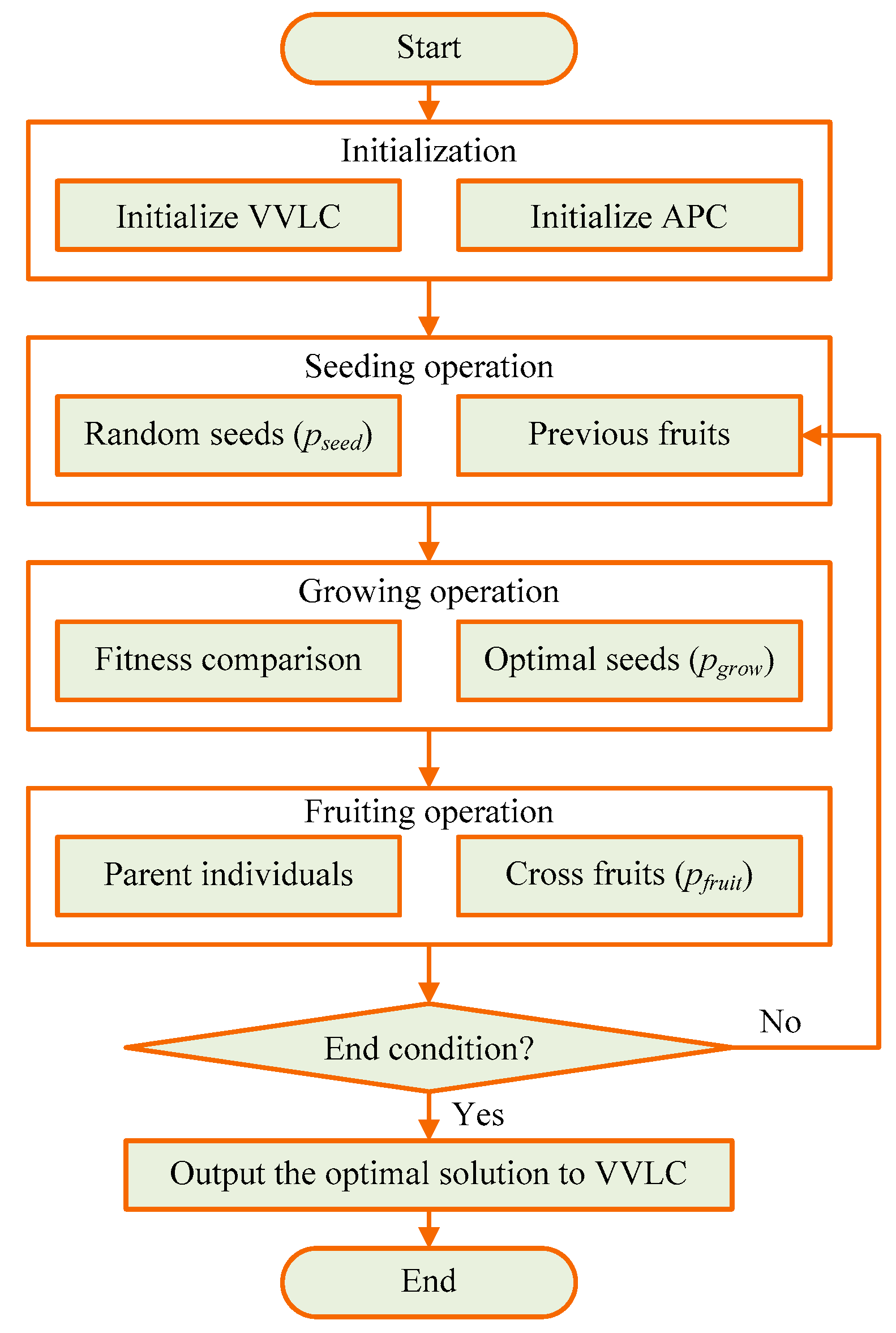
- To address the multi-objective optimization problem in time-sensitive VVLC flows, an improved artificial plant community (APC) algorithm [15] is proposed, with enhanced global search and local search capabilities. By randomly seeding, the global search ability is improved, and by giving the optimal plant individuals more fruiting opportunities, the local search ability is enhanced. This heuristic method intelligently determines whether efficient schedules may be used or searches for optimal scheduling solutions.
- To test the performance, we propose a benchmark test set and conduct a series of benchmark experiments for VVLC flow scheduling. The outcomes of the experiments show that the proposed APC algorithm can efficiently ensure a low makespan and delay, a high schedulable ratio and bandwidth utilization, quick response times, and low computation overheads.
2. Related Works
3. Problem Description
3.1. Notation Definition
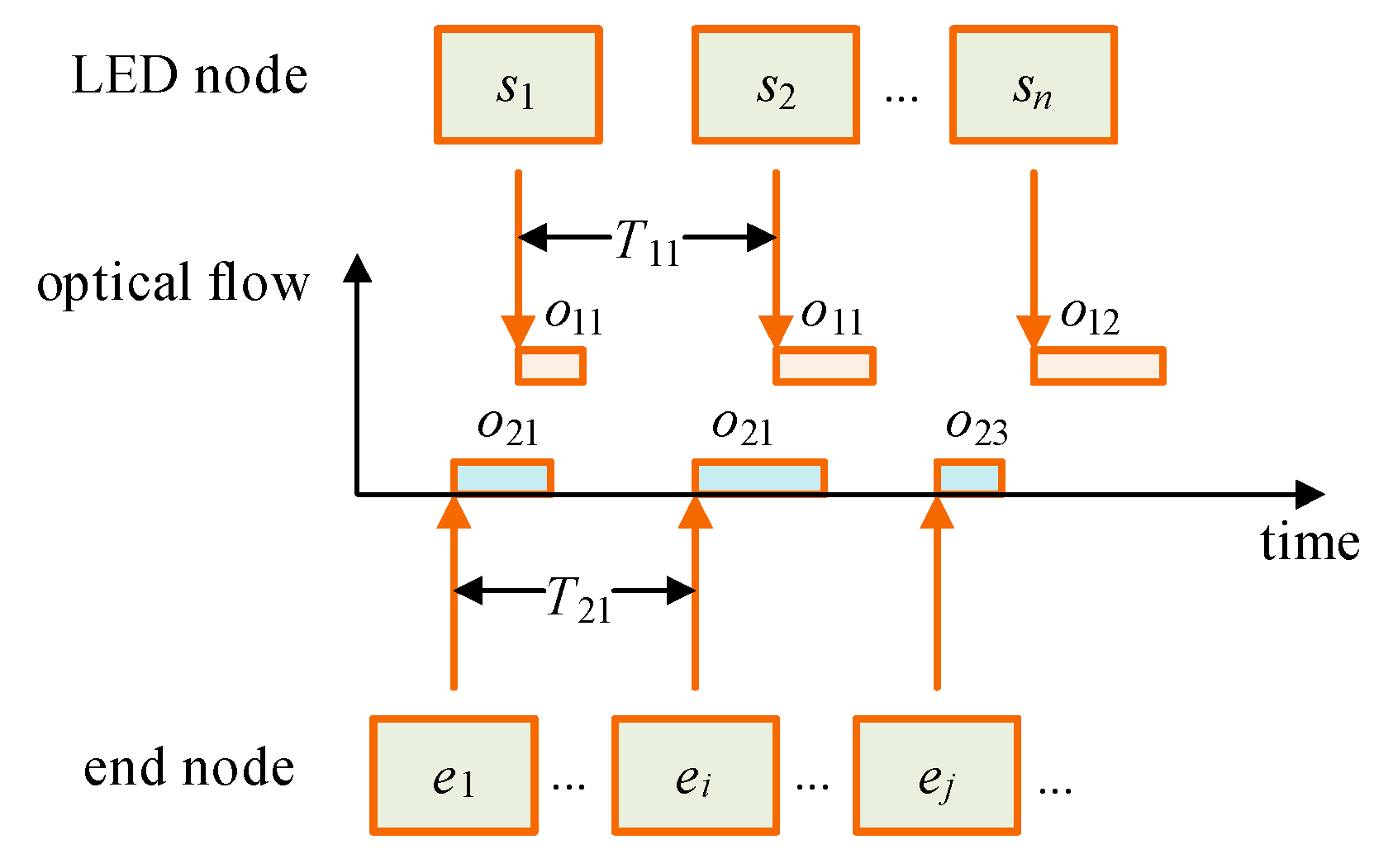
3.2. Optical Flow Scheduling Model of VVLC
3.3. Conflicts Between Optical Flows
3.4. Multi-Objective Optimization Model of VVLC
3.5. Integer Solution Space of VVLC
4. An Improved Artificial Plant Community Algorithm
4.1. Methodologies
4.2. Static APC Scheduling
| Algorithm 1. Static APC scheduling | |
| Input: , , , , , , . | |
| Set: , . | |
| Output: . | |
| 1: | |
| 2: | then |
| 3: | |
| 4: | else |
| 5: | |
| 6: | } |
| 7: | |
| 8: | |
| 9: | |
| 10: | |
| 11: | |
| 12: | |
| 13: | |
| 14: | then return to line 5 |
| 15: | end if |
| 16: | end for |
| 17: | |
4.3. Dynamic APC Scheduling
| Algorithm 2. Dynamic APC Scheduling | |
| , , , , , , . | |
| , . | |
| . | |
| 1: | |
| 2: | |
| 3: | |
| 4: | |
| 5: | i |
| 6: | |
| 7: | |
| 8: | |
| 9: | |
| 10: | |
| 11: | |
| 12: | |
| 13: | |
| 14: | then return to line 2 |
| 15: | end for |
| 16: | |
5. Simulation Results and Analysis
5.1. Experiment Setup
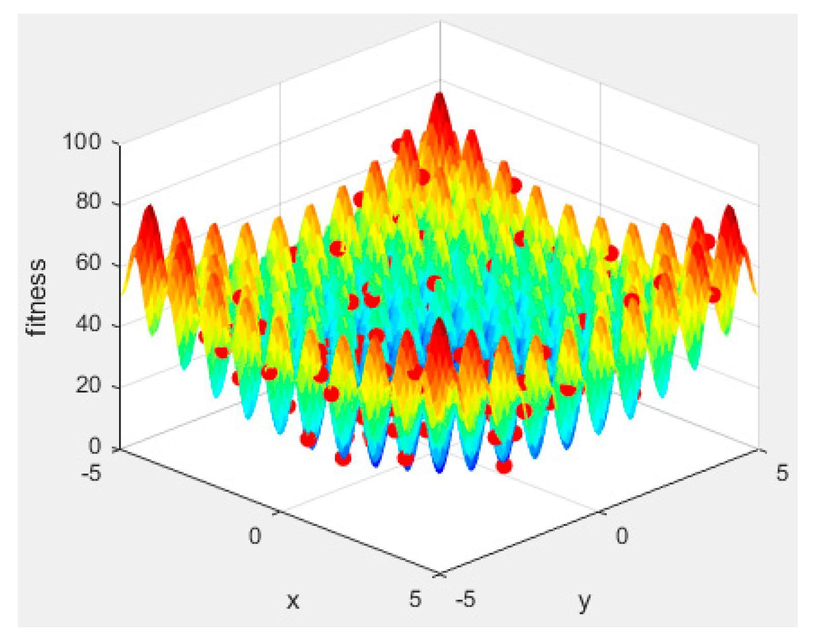
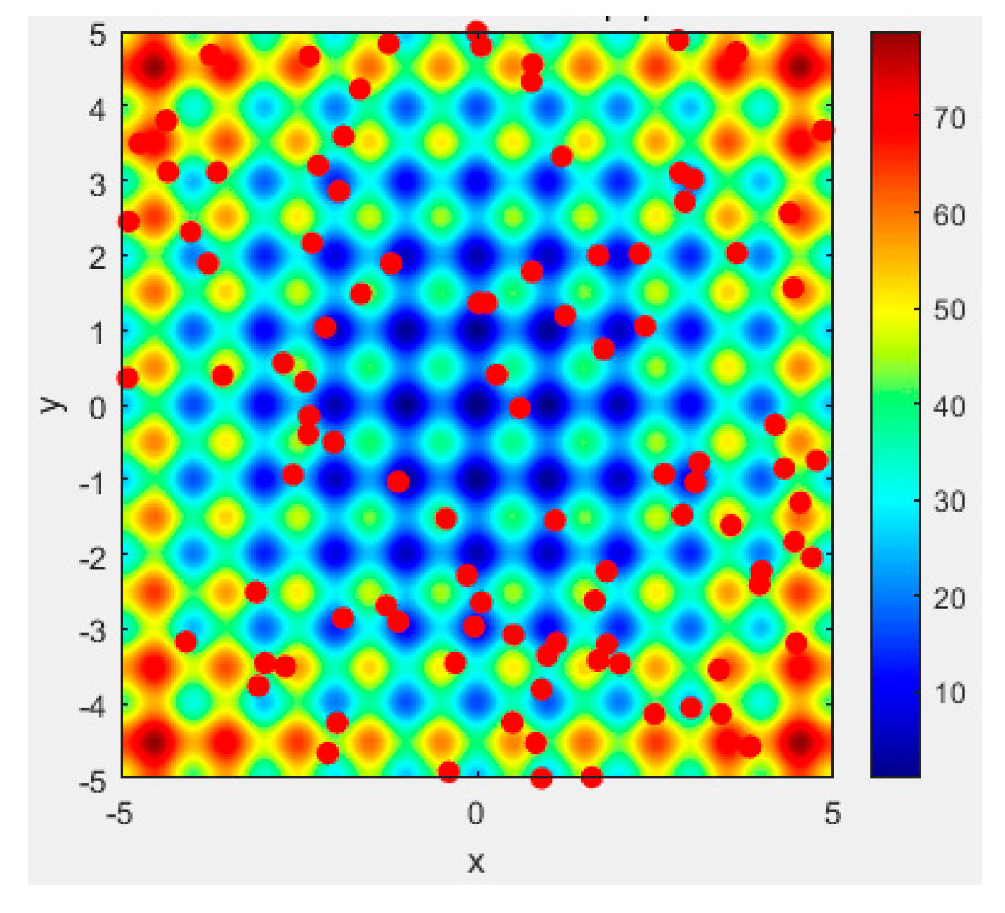
5.2. Benchmark Test of the APC Algorithm
5.3. Performance Comparison
5.4. Discussion
6. Conclusions
Author Contributions
Funding
Institutional Review Board Statement
Informed Consent Statement
Data Availability Statement
Acknowledgments
Conflicts of Interest
References
- Jing, X.; Wu, Y.; Yu, F.; Xu, Y.; Wang, X. Reconfigurable intelligent surface-aided security enhancement for vehicle-to-vehicle visible light communications. Photonics 2024, 11, 1151. [Google Scholar] [CrossRef]
- Sharda, P. Next generation based vehicular visible light communications: A novel transmission scheme. IEEE Trans. Veh. Technol. 2024, 73, 16735–16743. [Google Scholar] [CrossRef]
- Wang, J.; Luo, H.; Ruby, R.; Liu, J.; Wang, S.; Wu, K. Enabling reliable water–air direct optical wireless communication for uncrewed vehicular networks: a deep reinforcement learning approach. IEEE Trans. Veh. Technol. 2024, 73, 11470–11486. [Google Scholar] [CrossRef]
- Li, Y.C.; Wu, L.; Zhang, Z.C.; Dang, J.; Zhu, B.C.; Zhang, X.C.; Wu, Y.P. Sensing assisted optical wireless communication for UAVs. IEEE Trans. Veh. Technol. 2024, 73, 18620–18634. [Google Scholar] [CrossRef]
- Zadobrischi, E. Traffic and vehicle management in roundabouts through systems based on dedicated short-range communications and visible light communications. Electronics 2025, 14, 317. [Google Scholar] [CrossRef]
- Bu, F.F.; Luo, H.J.; Ma, S.S.; Li, X.; Ruby, R.; Han, G.J. AUV-aided optical-acoustic hybrid data collection based on deep reinforcement learning. Sensors 2023, 23, 578. [Google Scholar] [CrossRef]
- Pointurier, Y.; Benzaoui, N.; Lautenschlaeger, W.; Dembeck, L. End-to-end time-sensitive optical networking: Challenges and solutions. J. Light. Technol. 2019, 37, 1732–1741. [Google Scholar] [CrossRef]
- Zeng, H.S.; Zhang, C.X.; Yi, X.S.; Xiong, R. Heuristic fragmentation-aware scheduling for a multicluster time-sensitive passive optical LAN. Opt. Fiber Technol. 2021, 66, 102662. [Google Scholar] [CrossRef]
- Peng, Y.F.; Shi, B.X.; Jiang, T.G.; Tu, X.D.; Xu, D.; Hua, K. A survey on in-vehicle time-sensitive networking. IEEE Internet Things J. 2023, 10, 14375–14396. [Google Scholar] [CrossRef]
- Xu, Y.L.; Shang, J.; Tang, H. Recent trends of in-vehicle time sensitive networking technologies, applications and challenges. China Commun. 2023, 20, 30–55. [Google Scholar] [CrossRef]
- Li, J.; Bose, S.K.; Shen, G.X. Cooperative resource scheduling for time-sensitive services in an integrated XGS-PON and Wi-Fi 6 network. IEEE Commun. Lett. 2022, 26, 1338–1342. [Google Scholar] [CrossRef]
- Su, C.; Zhang, J.W.; Ji, Y.F. Time-aware deterministic bandwidth allocation scheme in TDM-PON for time-sensitive industrial flows. J. Opt. Commun. Netw. 2023, 15, 255–267. [Google Scholar] [CrossRef]
- Waqar, M.; Mustafa, M.U.; Jabeen, F.; Shah, S.A. Performance improvement of time-sensitive fronthaul networks in 5G Cloud-RANs using reinforcement learning-based scheduling scheme. IEEE Access 2024, 12, 59756–59770. [Google Scholar] [CrossRef]
- Wang, N.; Liu, J.F.; Lu, J.; Zeng, X.Y.; Zhao, X.Y. Low-delay layout planning based on improved particle swarm optimization algorithm in 5G optical fronthaul network. Opt. Fiber Technol. 2021, 67, 102736. [Google Scholar] [CrossRef]
- Cai, Z.; Ma, Z.; Zuo, Z.; Xiang, Y.; Wang, M. An image edge detection algorithm based on an artificial plant community. Appl. Sci. 2023, 13, 4159. [Google Scholar] [CrossRef]
- Wei, T.; Lin, T.; Huang, N.; Fu, C.; Liu, X.; Su, L.; Tang, L.; Hu, Q.; Gong, C. Multi-user scheduling and channel characteristics for water-to-air unmanned vehicular visible light communication. IEEE Trans. Veh. Technol. 2024, 73, 18705–18718. [Google Scholar] [CrossRef]
- Di, Y.; Xu, A.; Chen, L.K. Performance enhancement via real-time image-based beam tracking for WA-OWC with dynamic waves and mobile receivers. J. Light. Technol. 2024, 42, 6671–6678. [Google Scholar] [CrossRef]
- Yang, W.; Liu, H.; Cheng, G. Modeling and performance study of vehicle-to-infrastructure visible light communication system for mountain roads. Sensors 2024, 24, 5541. [Google Scholar] [CrossRef]
- Singh, K.D.; Sood, S.K. QoS-aware optical fog-assisted cyber-physical system in the 5G ready heterogeneous network. Wirel. Pers. Commun. 2021, 116, 3331–3350. [Google Scholar] [CrossRef]
- Li, Y. Quality of service improvement in fiber-wireless networks using a fuzzy-based nature-inspired algorithm. Photon. Netw. Commun. 2022, 44, 82–89. [Google Scholar] [CrossRef]
- Zhu, W.; Yang, X.; Wu, T.Y.; Qiu, Y. A routing algorithm for underwater acoustic-optical hybrid wireless sensor networks based on intelligent ant colony optimization and energy-flexible global optimal path selection. IEEE Sens. J. 2024, 24, 17116–17126. [Google Scholar] [CrossRef]
- Vyas, U. Deterministic lightpath scheduling and routing in elastic optical networks. Wirel. Pers. Commun. 2022, 124, 1593–1607. [Google Scholar] [CrossRef]
- Li, B.Q.; Zhu, Y.; Liu, Q.; Yao, X.X. Development of deterministic communication for in-vehicle networks based on software-defined time-sensitive networking. Machines 2024, 12, 816. [Google Scholar] [CrossRef]
- Mowla, M.M.; Ahmad, I.; Habibi, D.; Phung, Q.V.; Zahed, M.I.A. Green traffic backhauling in next generation wireless communication networks incorporating FSO/mmWave technologies. Comput. Commun. 2022, 182, 223–237. [Google Scholar] [CrossRef]
- Shin, H.; Baek, S.; Song, Y. Multidimensional beam optimization in underwater optical wireless communication based on deep reinforcement learning. IEEE Internet Things J. 2024, 11, 28623–28634. [Google Scholar] [CrossRef]
- Kamalakis, T.; Dogkas, L.; Simou, F. Optimization of a discrete multi-tone visible light communication system using a mixed-integer genetic algorithm. Opt. Commun. 2021, 485, 126741. [Google Scholar] [CrossRef]
- Arya, S.; Chung, Y.H. Artificial bee colony based iterative heuristic signal detection technique for optical wireless communications. IEEE J. Quantum Electron. 2023, 59, 8000311. [Google Scholar] [CrossRef]
- Singh, P.; Prakash, S. Implementation of marin predators algorithm for optimizing the position of multiple optical network units in fiber wireless access networks. Opt. Fiber Technol. 2022, 72, 102971. [Google Scholar] [CrossRef]
- Vieira, M.; Galvão, G.; Vieira, M.A.; Vestias, M.; Louro, P.; Vieira, P. Integrating visible light communication and AI for adaptive traffic management: a focus on reward functions and rerouting coordination. Appl. Sci. 2024, 15, 116. [Google Scholar] [CrossRef]
- Cai, Z.; Du, J.; Huang, T.; Lu, Z.; Liu, Z.; Gong, G. Energy-efficient collision-free machine/AGV scheduling using vehicle edge intelligence. Sensors 2024, 24, 8044. [Google Scholar] [CrossRef]
- Cai, Z.; Du, X.; Huang, T.; Lv, T.; Cai, Z.; Gong, G. Robotic edge intelligence for energy-efficient human–robot collaboration. Sustainability 2024, 16, 9788. [Google Scholar] [CrossRef]
- Lu, Y.; Liu, Y.; Yang, S.X.; Hua, Q.; Sangaiah, A.K.; Yu, K. An intelligent deterministic scheduling method for ultralow latency communication in edge enabled industrial internet of things. IEEE Trans. Ind. Inf. 2023, 19, 1756–1767. [Google Scholar] [CrossRef]
- Li, P.; Wei, X.; Tang, X.; Deng, J.; Xu, J. UAV-assisted free space optical communication system with decode-and-forward relaying. IEEE Trans. Veh. Technol. 2024, 73, 14102–14112. [Google Scholar] [CrossRef]
- Zhang, Z.; Wu, Q.; Fan, P.; Cheng, N.; Chen, W.; Letaief, K.B. DRL-based optimization for AoI and energy consumption in C-V2X enabled IoV. IEEE Trans. Green Commun. Netw. 2025. [Google Scholar] [CrossRef]
- P60802/D3.4, May 2025 - IEC/IEEE Draft International Standard Time-Sensitive Networking Profile for Industrial Automation. Date of Publication: 22 May 2025, Electronic ISBN: 979-8-8557-2246-8. Available online: https://ieeexplore.ieee.org/servlet/opac?punumber=11014762 (accessed on 7 July 2025).
- IEEE Std 802.15.7a 2024; IEEE Standard for Local and Metropolitan Area Networks—Part 15.7: Short Range Optical Wireless Communications Amendment 1: Higher Rate, Longer Range Optical Camera Communication (OCC). IEEE Computer Society: Washington, DC, USA, 2025.


| Notation | Explanation |
|---|---|
| The VVLC nodes | |
| A set of optical flows | |
| The period of an optical flow | |
| The greatest common divisor of periods for the optical flows | |
| The LED node number in TSON | |
| The end node number in TSON | |
| An optical flow from a node i to a node j | |
| The bandwidth of an optical flow | |
| The bandwidth of the directed edge | |
| Transfer time for a single packet in an optical flow | |
| The departure time of the 1st packet in an optical flow | |
| The arrival time of the 1st packet in an optical flow | |
| The packet processing time of an optical flow in the LED node | |
| Transfer power for a single packet in an optical flow | |
| The packet processing power of an optical flow | |
| The energy consumption of an optical flow | |
| The energy consumption of the directed edge | |
| Accumulated delay | |
| The delay constraints for the optical flows in O | |
| Accumulated jitter | |
| The jitter constraints for the optical flows in O |
| Optical Flow Number | Cycles T (ms) | Ratios | Packet Sizes (Byte) |
|---|---|---|---|
| 100 | (2.0, 1.0, 0.6, 0.3, 0.2, and 0.1) | 1:2:2:2:2:1 | 32 to 256 |
| 200 | (2.0, 1.0, 0.6, 0.3, 0.2, and 0.1) | 1:2:3:2:3:1 | 32 to 256 |
| 300 | (2.0, 1.0, 0.6, 0.3, 0.2, and 0.1) | 1:3:2:3:2:1 | 32 to 256 |
| 400 | (2.0, 1.0, 0.6, 0.3, 0.2, and 0.1) | 2:2:3:1:3:1 | 32 to 256 |
| 500 | (2.0, 1.0, 0.6, 0.3, 0.2, and 0.1) | 3:3:3:3:2:1 | 32 to 256 |
| Method | Number of Optical Flows | Mean | |||||
|---|---|---|---|---|---|---|---|
| 100 | 200 | 300 | 400 | 500 | |||
| APC | Makespan (s) | 0.165 | 0.238 | 0.347 | 0.475 | 0.572 | 0.359 |
| Accumulated delay (microseconds) | 25.6 | 38.4 | 52.2 | 64.3 | 74.5 | 51.0 | |
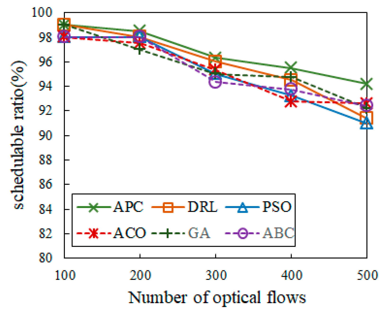
| Schedulable ratio (%) | 99.000 | 98.500 | 96.333 | 95.500 | 94.200 | 96.706 | |
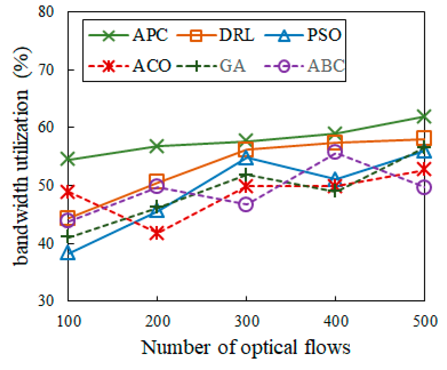
| Bandwidth utilization (%) | 54.545 | 56.768 | 57.636 | 58.947 | 61.946 | 57.9684 | |
| Solution time (s) | 5.682 | 6.491 | 7.576 | 8.848 | 9.682 | 7.656 | |
| DRL | Makespan (s) | 0.203 | 0.257 | 0.356 | 0.488 | 0.594 | 0.3796 |
| Accumulated delay (microseconds) | 28.1 | 39.5 | 55.3 | 64.8 | 77.2 | 52.98 | |
| Schedulable ratio (%) | 99.000 | 98.000 | 96.000 | 94.500 | 91.400 | 95.780 | |
| Bandwidth utilization (%) | 44.334 | 50.583 | 56.179 | 57.377 | 58.043 | 53.3032 | |
| Solution time (s) | 27.794 | 33.610 | 47.543 | 51.661 | 67.794 | 45.6804 | |
| PSO | Makespan (s) | 0.235 | 0.286 | 0.365 | 0.548 | 0.621 | 0.411 |
| Accumulated delay (microseconds) | 34.3 | 43.8 | 56.4 | 69.2 | 81.0 | 56.94 | |
| Schedulable ratio (%) | 98.000 | 98.000 | 95.000 | 93.250 | 91.000 | 95.05 | |
| Bandwidth utilization (%) | 38.297 | 45.614 | 54.794 | 51.094 | 56.000 | 49.1598 | |
| Solution time (s) | 6.015 | 6.432 | 7.691 | 8.946 | 10.015 | 7.820 | |
| ACO | Makespan (s) | 0.174 | 0.311 | 0.402 | 0.560 | 0.668 | 0.423 |
| Accumulated delay (microseconds) | 27.8 | 47.1 | 57.5 | 68.9 | 76.7 | 55.6 | |
| Schedulable ratio (%) | 98.000 | 97.500 | 95.330 | 92.750 | 92.600 | 95.236 | |
| Bandwidth utilization (%) | 48.913 | 41.801 | 49.875 | 49.910 | 52.711 | 48.642 | |
| Solution time (s) | 5.994 | 6.733 | 7.692 | 9.012 | 9.994 | 7.885 | |
| GA | Makespan (s) | 0.219 | 0.280 | 0.386 | 0.571 | 0.627 | 0.417 |
| Accumulated delay (microseconds) | 26.2 | 42.0 | 58.6 | 73.4 | 75.3 | 55.1 | |
| Schedulable ratio (%) | 99.000 | 97.000 | 95.000 | 94.750 | 92.200 | 95.590 | |
| Bandwidth utilization (%) | 41.095 | 46.263 | 51.813 | 49.036 | 56.542 | 48.9498 | |
| Solution time (s) | 5.878 | 6.774 | 7.705 | 8.927 | 9.878 | 7.832 | |
| ABC | Makespan (s) | 0.205 | 0.261 | 0.428 | 0.503 | 0.704 | 0.420 |
| Accumulated delay (microseconds) | 31.7 | 42.5 | 61.9 | 66.7 | 84.6 | 57.48 | |
| Schedulable ratio (%) | 98.000 | 98.000 | 94.333 | 93.750 | 92.400 | 95.296 | |
| Bandwidth utilization (%) | 43.902 | 49.808 | 46.728 | 55.666 | 49.645 | 49.1498 | |
| Solution time (s) | 6.106 | 6.551 | 7.667 | 9.113 | 10.106 | 7.9086 | |
Disclaimer/Publisher’s Note: The statements, opinions and data contained in all publications are solely those of the individual author(s) and contributor(s) and not of MDPI and/or the editor(s). MDPI and/or the editor(s) disclaim responsibility for any injury to people or property resulting from any ideas, methods, instructions or products referred to in the content. |
© 2025 by the authors. Licensee MDPI, Basel, Switzerland. This article is an open access article distributed under the terms and conditions of the Creative Commons Attribution (CC BY) license (https://creativecommons.org/licenses/by/4.0/).
Share and Cite
Cai, Z.; Lei, S.; Li, J.; Yu, C.; Liu, J.; Gong, G. A Heuristic Optical Flow Scheduling Algorithm for Low-Delay Vehicular Visible Light Communication. Photonics 2025, 12, 693. https://doi.org/10.3390/photonics12070693
Cai Z, Lei S, Li J, Yu C, Liu J, Gong G. A Heuristic Optical Flow Scheduling Algorithm for Low-Delay Vehicular Visible Light Communication. Photonics. 2025; 12(7):693. https://doi.org/10.3390/photonics12070693
Chicago/Turabian StyleCai, Zhengying, Shumeng Lei, Jingyi Li, Chen Yu, Junyu Liu, and Guoqiang Gong. 2025. "A Heuristic Optical Flow Scheduling Algorithm for Low-Delay Vehicular Visible Light Communication" Photonics 12, no. 7: 693. https://doi.org/10.3390/photonics12070693
APA StyleCai, Z., Lei, S., Li, J., Yu, C., Liu, J., & Gong, G. (2025). A Heuristic Optical Flow Scheduling Algorithm for Low-Delay Vehicular Visible Light Communication. Photonics, 12(7), 693. https://doi.org/10.3390/photonics12070693