3.1. Line Spread Function
The line spread function (LSF) serves as a fundamental descriptor of optical system performance for line source imaging [
16,
17]. It represents the light intensity distribution along a specific direction (usually perpendicular to the line light source) after the line light source is imaged by an optical system. Under normal circumstances, the LSF is mathematically derived from the Point Spread Function (PSF) through the integral relationship expressed in Equation (
1).
Here, denotes the Point Spread Function (PSF) characterizing the optical system’s spatial response to a point source, indicates the coordinate position of the response in the readout data. The LSF is obtained by integrating the PSF along the longitudinal axis (y-axis) parallel to the line source’s extended dimension. In this coordinate framework, the transversal x-axis defines the measurement direction of the LSF, while the longitudinal y-axis coincides with the geometric orientation of the line source.
The line spread functions (LSFs) across distinct spectral bands in multiple image slicers can be derived from slit-enhanced imagery acquired at the object plane. For each image slicer array response, a scanning frame protocol sequentially isolates effective data points along the image rows, followed by estimation of the LSF parameter through Gaussian fitting upon valid identification of the data point.
Common methodologies for characterizing LSFs encompass Gaussian profile fitting, Lorentzian distribution modeling, polynomial regression, Fermi function approximation, and composite function synthesis. The Gaussian and Lorentzian approaches demonstrate optimal efficacy for symmetric datasets with smooth curvature profiles, whereas polynomial decomposition has proven suitable for complex morphological distributions. Asymmetric data structures necessitate Fermi function implementation, while intricate LSF configurations require composite model integration. Empirical analysis of experimental response data reveals the superior suitability of Gaussian/Lorentzian paradigms for LSF reconstruction. The formula for the Gaussian fitting LSF is presented in Equation (
2), and the formula for the Lorentzian fitting LSF is presented in Equation (
3) [
18]. When processing experimental detector-readout image data, each slice’s signal response is processed individually. The pixel data fitting procedure, conducted row-by-row, incorporates both screening operations and regression analysis applied exclusively to integer-row pixel arrays. The fitting process establishes a precise correspondence between the column indices of response data in the detector readout image and the signal response values (voltage code values) at their corresponding pixel locations.
In the above formulas,
and
represent the signal response values and x represents the column index of the pixel in the detector readout image. In Equation (
2),
A is the height of the peak,
is the center position of the peak,
b is the bias term, and
is the standard deviation, which determines the width of the curve. In Equation (
3),
A is the height of the peak,
is the center position of the peak,
b is the bias term, and
is the half-width, which determines the width of the curve.
Table 1 quantitatively compares these two methodologies through three key metrics: mean root mean square error (RMSE, calculated as the square root of the mean squared difference between the measured intensity values at test points and the corresponding values predicted by the fitted LSF curve), average coefficient of determination (
), and successful fitting rows per image slicer group.
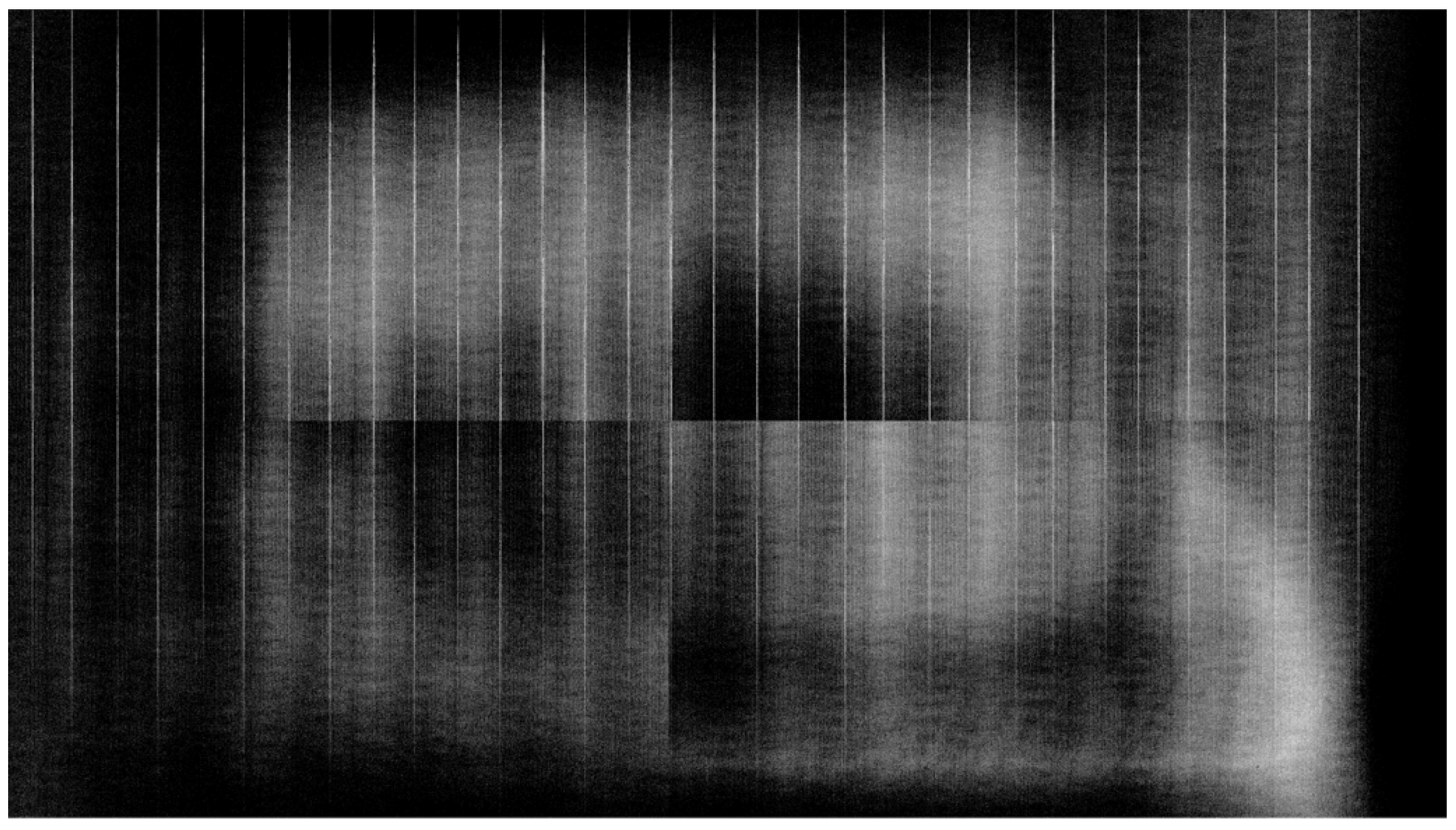
Table 1 presents a comparison of the performance of the Lorentzian and Gaussian fitting methods. The RMSE represents the root mean square deviation between the signal response values (voltage code values) at the original coordinate points and the predicted signal response values obtained from the fitted curve using the two methods at the input locations. Successful fitting rows refer to the number of rows in each image slicer that successfully fit a Gaussian curve and have a linearity greater than 0.94. The Lorentzian fitting method has a slightly smaller root mean square noise than the Gaussian fitting method. However, this slight advantage is offset by the fact that the number of successfully fitted curves using the Lorentzian method is significantly smaller than that of the Gaussian method. The number of fitted rows per group denotes the count of successfully fitted rows in each group. As the vertical direction of the detector’s response is the spectral dispersion direction, inserting a slit before the lens elicits a response from each band. Within the 440 nm to 600 nm range of the Hg-Ar lamp, each row corresponding to the bands in each group’s slicer response was fitted, and a slit position table for each band was generated, which was vital for subsequent calculations. A higher number of fitted rows enhances the subsequent processing precision; unresponsive bands require interpolation. This reflects the fitting method’s stability and applicability across data groups. Using the Lorentzian method results in fewer successfully fitted rows than the Gaussian method, implying a lower stability and applicability. Additionally, the Lorentzian method showed lower correlation. Thus, the Gaussian method offers better applicability and results in a more accurate LSF, proving to be superior, more reliable, and more effective for application. The halogen lamp response image obtained after placing a slit in front of the spectrometer lens can be seen in
Figure 7.
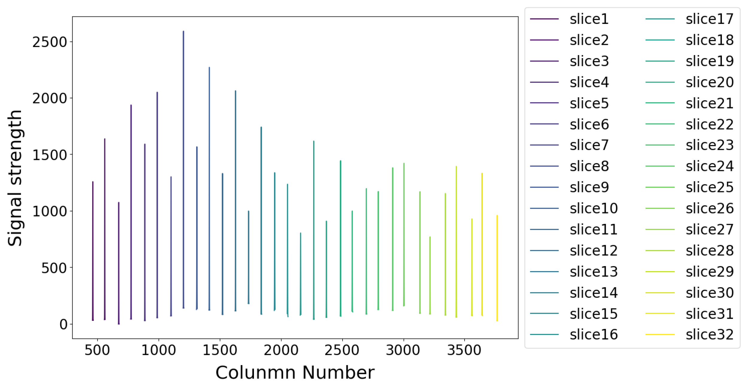
Figure 8 and
Figure 9 share the same coordinate system, with the horizontal axis indicating the detector column number and the vertical axis representing the pixel signal intensity.
Figure 9 presents the measured LSFs for all image slicer groups at 546.10 nm, corresponding to the spectral channel mapped by the integer-row pixel with nearest-neighbor interpolation to the characteristic 546.07 nm emission line of the Hg-Ar calibration source.
Figure 9 provides a magnified analysis of the first LSF curve from
Figure 8.
Figure 8 shows the peak response at 546.10 nm for all 32 slices (numbered 1 to 32 from left to right), with peak positions ranging from column 461.85 to 3767.10. The horizontal axis represents the column number of the detector, and the vertical axis represents the pixel response value. Due to optical system attenuation, the response of each slice varies. The LSF for each slice has a full width at half maximum (FWHM) of 1.32 to 2.38 pixels, averaging 1.73 pixels.
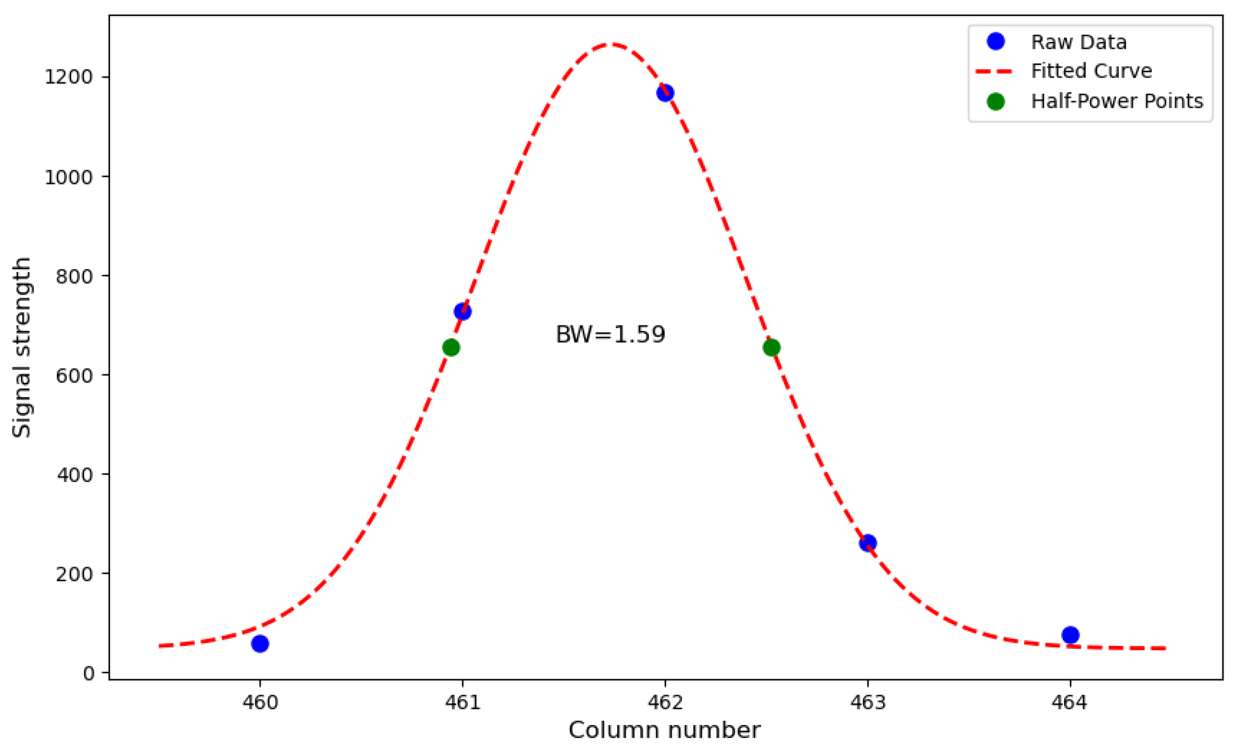
Figure 9 displays an enlarged view of the fitting curve for slice 1 (the leftmost slice in
Figure 8), where the peak is located at column 461.85 and the full width at half maximum is 1.59 pixels. The horizontal axis represents the column number of the detector, and the vertical axis represents the pixel response value (digital number).
3.2. Confirmation of Specific Spectral Segment Positioning Points
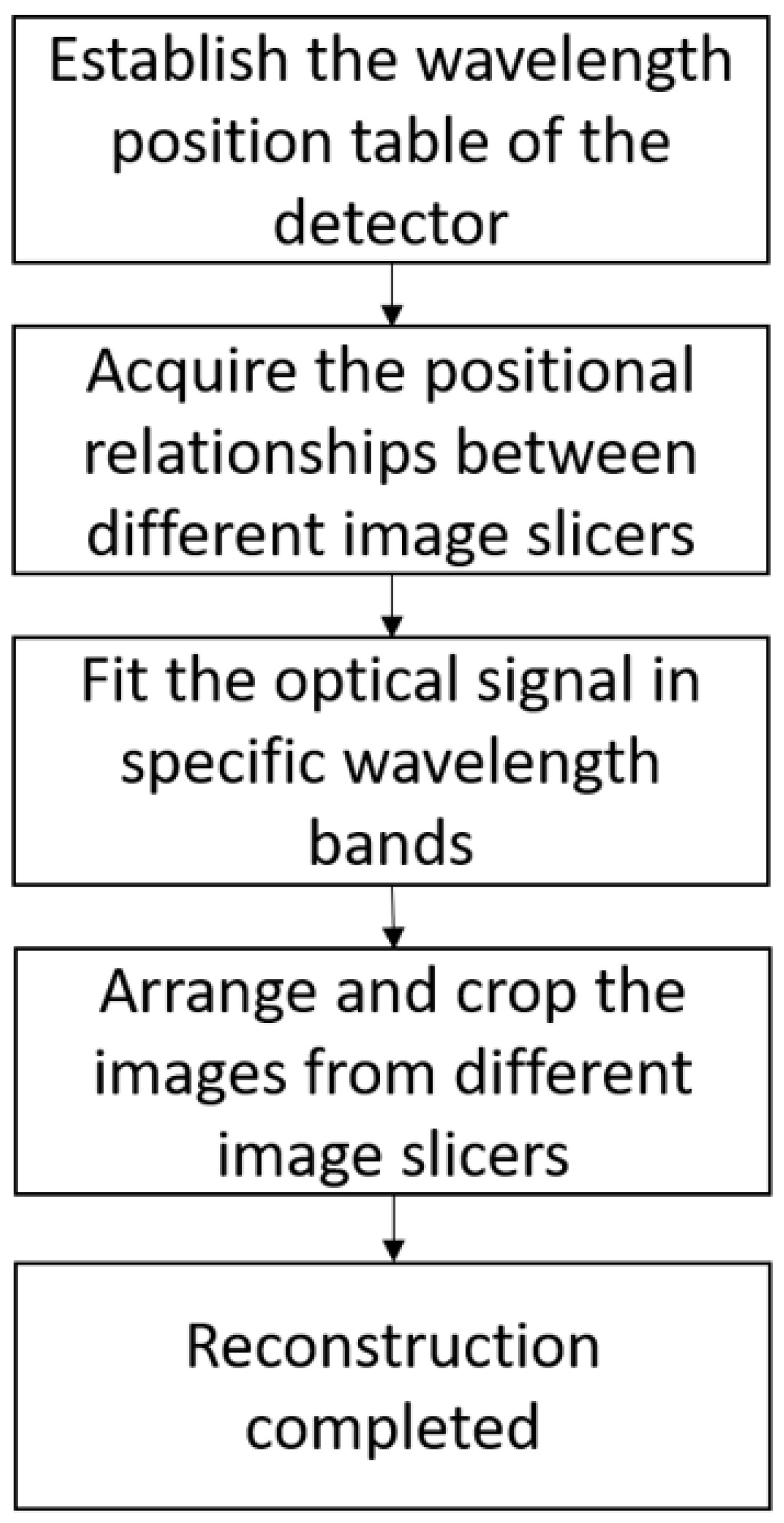
After determining the positions of the selected spectral bands in the 32 slices through the wavelength calibration table, the 32 sets of positions need to be aligned into a new common coordinate system. The main purpose of this section is to obtain a set of point coordinates that serve as positioning points. These coordinates establish a connection between the different sub-fields from the image slicer for the same spectral band. This means that these point coordinates help combine the 32 sub-fields into a 2D field-of-view image at the spectrometer lens. Aiming at the simultaneous response characteristics of spatial and spectral dimensions produced by the image slicer technology in spatial IFSs, this study proposes a sub-pixel-level interlinking positioning method. This method uses spatial coordinate data generated by a modulated sub-field slit (smaller than 1 instantaneous field-of-view) as input, combines it with spectral coordinate data from the wavelength calibration table, and performs initial data screening via a dynamic sliding window strategy; this strategy reduces the influence of distal data values on interpolation fitting. A bidirectional mapping model is constructed based on quintic spline interpolation technology. An adaptive smoothing coefficient is used to balance the model complexity and noise suppression requirements. To further enhance positioning stability, a composite optimization objective function including second derivative constraints is designed, integrating multiple constraints such as curvature smoothness, and robust penalty terms, ultimately outputting stable intersection coordinates that meet sub-pixel-level accuracy requirements. The positioning method process is shown in
Figure 10. In this section, the algorithm selects the spatial coordinate data of the characteristic spectral line at 546.07 nm as the spectral reference and combines it with the spatial information formed by the sub-field slit modulation as input to achieve sub-pixel-level positioning for each image slicer group.
As the incident field is split into 32 sub-fields by the image slicer, it is necessary to locate the alignment markers for each sub-field. The first sub-field is used as an example in the following description, while the remaining sub-fields follow an identical processing method. Firstly, from
Figure 10, it can be seen that there are two inputs: the response position information
of a specific spectral segment in each slice of the image slicer obtained from the detector readout image via the wavelength calibration table, and the centroid position
of the halogen lamp’s spectral response, acquired through a slit-apertured optical configuration positioned at the spectrometer’s entrance port. For these two sets of positions, response functions of
and
are established. The function
represents the response position information of each slice of the image slicer in a specific spectral segment obtained from the detector readout image via the wavelength calibration table. Here, the input
is an integer and denotes the column number of the detector readout image and the input
denotes the row number. The function
represents the response position of each slice of the integral field spectrograph’s before introduction of the slit in response to the halogen lamp, which can be determined by the peak positions of each slice at 440 nm to 600 nm (the spectral range of the halogen lamp), as described in
Section 3.1. Here, the input
is an integer and denotes the row number of the detector readout image and the input
denotes the column number. Theoretically, these two functions for each set of slices will have an intersection point.
To determine this intersection point, it is necessary to interpolate the two sets of functions to find a common position. To filter out valid positional information from the two datasets, reducing workload and enhancing result accuracy, a characteristic point (the integer point closest to the two sets of positional information) first needs to be identified. Then, an asymmetric search region is established around this characteristic point to select positional information and subsequently, interpolation is required to obtain the intersection of the two sets of input data. Given the shape of the two sets of positional information, a spline interpolation method suitable for one-dimensional data processing was chosen. Typically, cubic spline interpolation is commonly used for curve fitting problems [
19]; however, it may not suffice in cases where high smoothness and curvature are required. Quintic spline interpolation has advantages in such scenarios [
20,
21]. While cubic spline ensures continuity of the first derivative, quintic spline achieves continuity of the second derivative, ensuring smooth curvature changes. Quintic spline interpolation also provides a higher precision and strong adaptability to noise. Quintic B-spline interpolation further enhances these advantages [
22]. It offers a high precision and lower computational costs. It is capable of determining the solution providing an estimated solution at any mesh point in the domain. Given these advantages, we choose quintic B-spline to construct the functions
and
, which are shown in Equations (
4) and (
5), respectively.
In Equations (
4) and (
5),
represents the response position in the detector readout data for a specific wavelength band.
represents the spatial coordinates in the detector focal plane data, measured after light from the halogen lamp passes through the pre-slit assembly of the spectrograph lens.
and
represent the coordinate weights of the control points, corresponding to the fitting coefficients in their respective basis functions. These weights are optimized via the least squares method to approximate the input data points
and
with a spline curve. Adjusting these weights modulates the control points’ influence on the curve geometry, thereby enhancing the fidelity of the data fitting. The quintic spline basis functions
and
are defined using the Cox–de Boor recursive formula, as shown in Equations (
6) and (
7).
In these formula,
and
are knot vectors. They determine the intervals over which the basis functions are non-zero and thus control the local influence of each control point. Knot vectors are typically chosen to be non-decreasing sequences of real numbers, and their values can affect the smoothness and continuity of the resulting spline curves. The functions
and
can be represented by
Figure 11. The function
can be represented by
Figure 11a, where the green points indicate the position of the spectral response at 546.07 nm, and the orange line represents the function constructed using a fifth-order B-spline. The function
can be represented by
Figure 11b, where the blue points indicate the position of the slit’s spatial response on the detector, and the blue line represents the function constructed using a fifth-order B-spline.
The objective function transforms the mathematical properties of quintic splines into a computable optimization problem through a closed-loop optimization framework, thus avoiding the need to solve for the intersection of two quintic spline functions, with its core coupling mechanism presented in Equation (
8).
In this formula, represents the horizontal residual that ensures consistency between the intersection’s x-coordinate (detector column) and the actual value. Similarly, denotes the vertical residual ensuring alignment of the y-coordinate (detector row) at the intersection with its true position. Absolute distances are adopted here to prevent sign-based error cancellation, which could otherwise produce false focal point coordinates by allowing positive and negative deviations to offset each other. These residuals together establish a dual closed-loop verification mechanism, effectively mitigating the cumulative impact of fitting deviations in single directions. When the value of E(x,y) is minimized, the positioning point (x,y) is obtained.
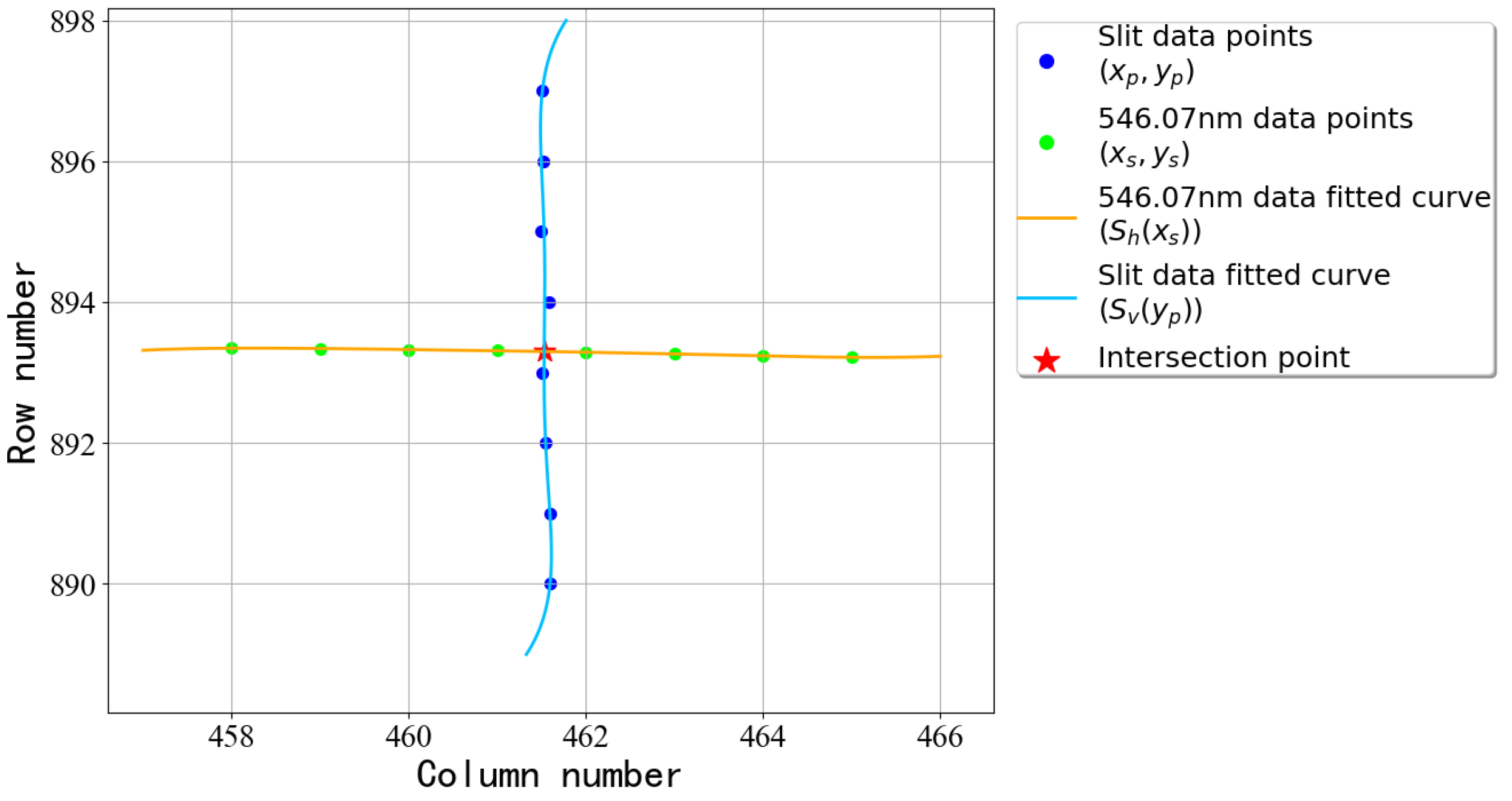
Figure 12 shows the positioning points of the first group of image slicers in the 546.07 nm band, with a focus on the fitting results of the center point. This figure includes specific data points and fitting curves, the localization point clearly demonstrates the positioning process.
Figure 12 presents the fitting results for 546.07 nm and the slit data of the first slice using a sub-pixel-level interconnect localization method. The blue dots show the position of 546.07 nm from the wavelength calibration table, with the fitted curve represented by the blue line. The green dots indicate the position mapped from the slit response, with its fitted curve in orange. The red dot marks the intersection point at (461.85689, 470.38038). From the figure, it can be observed that the calculated positioning points are accurate.
3.3. Image Slicer Group Alignment
Reconstructing the object–plane view of the lens requires integrating observation data from multiple spectral slice modules into a unified view. The position coordinates of each slice at a specific spectral segment can be obtained via a wavelength calibration table. Based on these coordinates, the signal response values for each position can be determined. Since the y-coordinate of each position is likely a fractional value, fitting using the spectral response values of integer pixel points is required to obtain the spectral response values at these sub-pixel locations.
For the laboratory data collected using a halogen lamp and a Hg-Ar lamp, the spectral dimension of the Hg-Ar lamp’s signal is used to extract intensity values at the selected spectral segments through Gaussian fitting. The halogen lamp response can be seen in
Figure 7. Due to the similar, continuous responses of adjacent pixels, the response at a certain band cannot be obtained through Gaussian fitting. Given the high spectral resolution of the spectrograph, spectral aliasing between bands is negligible. Therefore, a simple one-dimensional linear interpolation is adopted for initial fitting and reconstruction evaluation. This allows for the acquisition of signal response values for all position points of the 32 slice groups at specific spectral segments.
Next, a new coordinate system must be established to integrate the 32 slice groups. Initially, the 32 sets of one-dimensional data are combined from top to bottom according to their slicing order in the optical system. At this point, each row may contain a different number of pixels, and it is uncertain whether the pixels are correctly connected vertically. Therefore, the positioning points obtained from
Section 3.2 are used for verification. These positioning points are identified at the location of each slice and arranged linearly in the new coordinate system. Subsequently, each slice group is trimmed based on the shortest distance between its left and right boundaries and the positioning points. This process results in a well-organized two-dimensional field-of-view image.
The reconstructed images not only visualize data distribution characteristics but also establish a foundation for subsequent quantitative analysis. As representative examples,
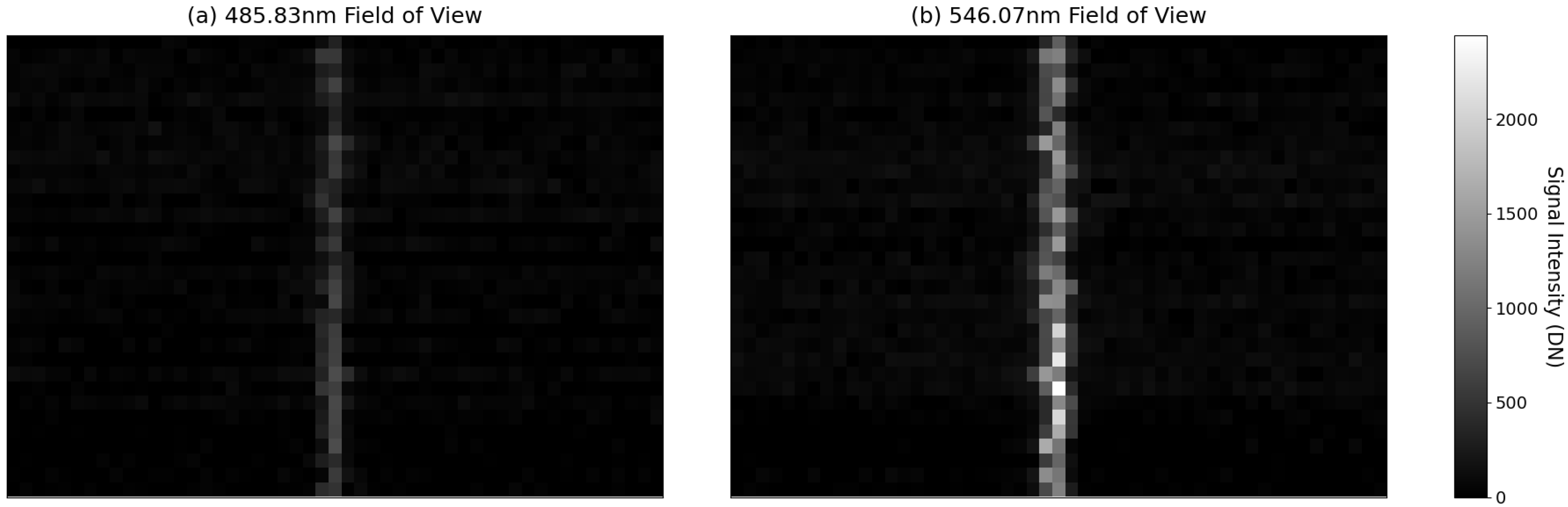
Figure 13 shows the 485.83 nm and 546.07 nm bands reconstructed using Quintic B-spline interpolation under halogen lamp illumination, with a slit installed in front of the spectrograph lens. Similarly,
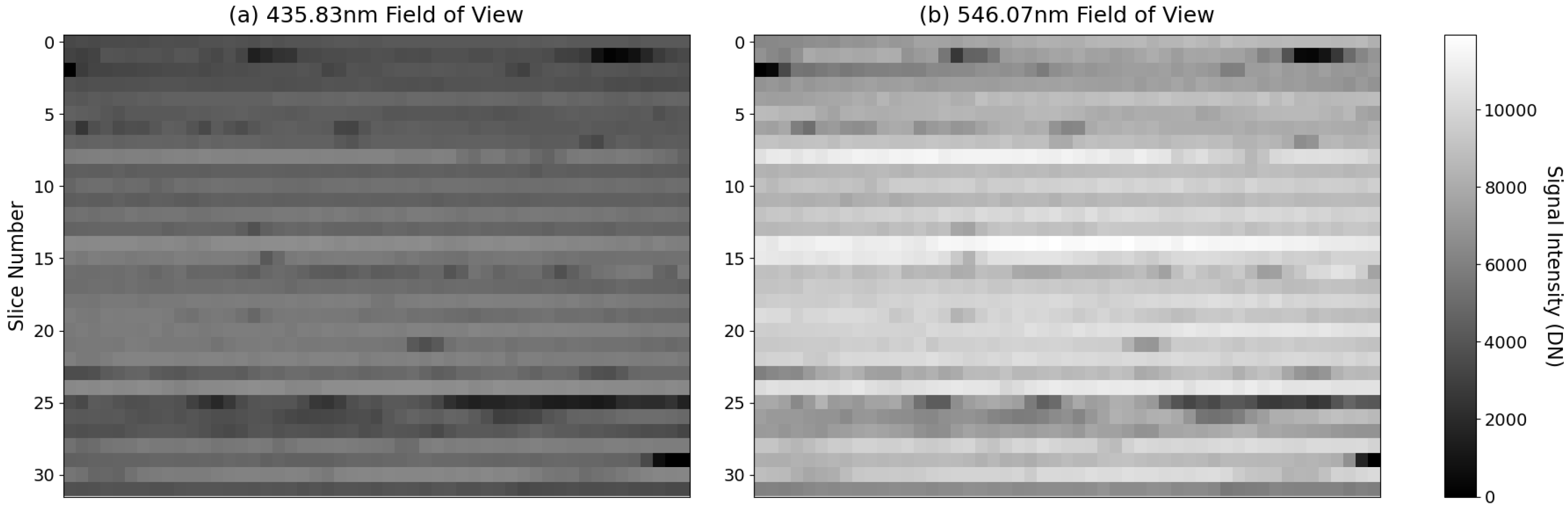
Figure 14 displays the 435.83 nm and 546.07 nm bands reconstructed with the same method under Hg-Ar lamp illumination. For a comprehensive method comparison,
Table 2 quantifies the positioning accuracy by showing the average pixel deviation between peak response positions and ground truth points across all rows in the field-of-view images of
Figure 13’s spectral bands, evaluating three interpolation methods: Quintic B-spline, Cubic B-spline, and Linear interpolation.
The offset in
Table 2 refers to the peak response positions of the slit in each pixel row compared to the positioning points. This offset should theoretically correspond to the horizontal ordinate of the positioning points in each slice from
Section 3.2. The results demonstrate that Quintic B-spline interpolation achieves the smallest deviation, followed by Cubic B-spline and Linear interpolation methods, with Quintic B-spline interpolation’s sub-0.25-pixel deviation validating the effectiveness of the proposed approach. In
Figure 13 and
Figure 14, red dots mark the 32 sub-pixel positioning points (not aligned with the pixel centers). The horizontal axis represents the one-dimensional data of the two-dimensional field-of-view segments from each slice, while the vertical axis represents the 32 slices of the image slicer.
Figure 13 displays the 2D field-of-view images of two spectral bands acquired with a slit installed in front of the spectrograph lens. The response signals are distributed across pixels adjacent to the positioned coordinates. Through the positioning point fitting algorithm, these coordinates are determined to be proximal to the true spectral peaks, which may not coincide with discrete pixel coordinates. In particular, strong responses at integer pixel positions are often located on either side of the actual peak position, consistent with the signal distribution shown in the image. This alignment validates the efficacy of our methodology.
In
Figure 14, the 2D field-of-view images of two spectral bands from the Hg-Ar lamp reveal that slice 25 exhibits a weaker response compared to other slices. This discrepancy likely stems from the higher optical path attenuation within this specific slice. When observing targets in this region, an extended integration time should be applied to enhance the response intensity. Additionally, the pixel-wise non-uniformity observed in the image requires correction based on responses at different energy levels.


