Combating Antimicrobial Resistance: Spectroscopy Meets Machine Learning

Abstract

One of the major health challenges that humans have been facing for the last few decades is antimicrobial resistance (AMR), where antibiotics stop responding to infections and, thereby, take a considerable amount of time to cure them while increasing mortality rates. There are various steps that have been taken by researchers and organizations to identify, cure, and prevent this urgent issue. Here, in this review, we have tried to illustrate how machine learning has been used with different spectroscopic analytical platforms—Raman spectroscopy (RS), Fourier-transform infrared spectroscopy (FTIR), and nuclear magnetic resonance (NMR)—to further accelerate the understanding and early detection of AMR. The combination of ML algorithms with advanced spectroscopic techniques delivers faster and deeper insights into the different mechanisms of bacterial resistance, delivering novel solutions.

1. Introduction

Antimicrobial resistance (AMR) is associated with major health challenges experienced in every part of the world. AMR reduces the efficacy of antibiotics and causes longer infection and high mortality risks in affected patients infected individuals. According to the World Health Organization (WHO), due to the global risk to human health and wellness, it is necessary to take action against AMR [1]. The primary reason for AMR has been reported to be the unregulated usage of various antibiotics. Antibiotics are easily available in different parts of the world, without prescription, resulting in an overuse and misuse of antibiotic medications [2]. Patients who fail to follow prescribed antibiotic instructions also contribute to the growth of resistance; as incomplete antibiotic therapy enables bacterial survival by encouraging tolerance against that specific antibiotic [3]. The development of new drugs requires long research times and high funding costs, leading to fewer innovations in drug discovery [4,5]. Additionally, to prevent bacterial infections in agricultural sectors while maximizing the productivity of livestock, antibiotics have been overused and as a result have entered the human food supply, further complicating the situation [4]. The WHO has disclosed that, on average, resistance development against a new antibiotic takes 2–3 years post market entry [6]. This explains the alarming scenario waiting for us unless we fail to adopt novel strategies to combat AMR soon. One of the main challenges of combating antimicrobial resistance lies in the economic dimensions of antibiotic development and deployment. Although it seems logical to develop new antibiotics to counter resistance to existing drugs, the process of discovering, testing, and approving a new antibiotic for clinical use demands a huge investment of time, skilled personnel, and funding.

Antimicrobial susceptibility testing (AST) can be performed through different methodologies for different clinical and research needs. Among them, microdilution [7] remains the benchmark method due to its precision in determining the minimum inhibitory concentrations (MICs), its high reproducibility, and its compatibility with different automated systems. It can generate detailed resistance profiles by testing multiple antibiotics across their different dilution ranges simultaneously. The gradient diffusion method, commonly known as the E-test, offers MIC readings from an antibiotic-coated strip placed on agar plates [8]. This method is more expensive, and interpreting the results is somewhat subjective between different clinicians. However, it is commonly used for testing fastidious or multidrug-resistant organisms. Meanwhile, disk diffusion (the Kirby–Bauer method) is considered a gold-standard method in routine diagnostics [8] because of its ease of use and affordability, despite being influenced by factors like agar composition and zone measurement variability by different clinicians. In parallel with these established approaches, many novel biophysical and optical techniques are reshaping the AST landscape. For example, dielectrophoresis (DEP) utilizes the motion of a bacterial population in non-uniform electric fields to separate viable and non-viable cells, thereby delivering a rapid, label-free analysis of different antibiotic potencies [9]. Optoelectronic sensors detect changes in optical properties like absorbance, reflectance, or refractive indices while monitoring bacterial responses to different antibiotics in real time [10]. These sensors can detect metabolic shifts, cell lysis, or biofilm dynamics with high sensitivity and speed, but due to the strain-specific signal interpretation and environmental variability, their adoption is currently limited.

Table 1. Comparison of conventional and emerging AST methods based on output type, turnaround time, automation potential, and limitations.

Method	Output	Time to Result	Automated Compatibility	Limitations
Microdilution	MIC	16–24 h	High	Labor-intensive, requires incubation
Gradient Diffusion (E-test)	MIC	16–24 h	Medium	Higher cost, subjective MIC reading
Disk Diffusion	Zone Diameter	16–24 h	Low	Qualitative, no MIC
Dielectrophoresis (DEP)	Viability	<1 h	Medium	Device complexity, sensitive to the ionic environment
Optoelectronic Sensors	Metabolic/Structural Changes	<1 h	High	Environmental sensitivity, complex fabrication

compares the traditional and some of the emerging AST methods on the basis of different parameters.

In addition to the traditional culture-based methods, various spectroscopic techniques have gained attention due to their ability to offer a rapid, label-free alternative for the study of bacterial composition and bacterial response to different antibiotic agents. However, these spectroscopic data are very much layered and complex to understand. This is where machine learning (ML) algorithms merge with spectroscopic data for the analysis plus interpretation of these multifaceted data layers, ensuring a speedy and accurate detection of normal and resistant bacteria [11]. There are several studies performed to extract information from pathogenic bacteria; for example, Ho et al. applied different ML algorithms to spot motifs and biomarkers related to bacterial resistance, which are extremely complicated to recognize manually [12]. Such a combination of ML algorithms with spectroscopic data increases the pace of the diagnostic process, thereby delivering effective treatment courses of action and helps in preventing further infection [13]. This review contributes a summary of various ML algorithms that have been employed to fight against the growing danger of antimicrobial resistance.

2. Spectroscopic Methods in AMR Detection

Spectroscopy is the study of the interaction between light and matter, offering a molecular-level understanding of the chemical composition, structural organization, and dynamic behavior of matter [14]. There are many spectroscopic methods, categorized based on unique aspects of radiation, interaction principle, resolution, and the nature of samples. In the following sections, we briefly give an overview of the primary spectroscopic methods that have been applied in exploring AMR.

2.1. Raman Spectroscopy

Raman spectroscopy is a powerful and non-invasive optical method that exploits laser light to scan a given sample (here, it is bacteria). This technique is based on the inelastic scattering of monochromatic light, where the shift in energy represents molecular vibrational modes within the sample [15]. These shifts offer insights into the chemical bonds and molecular environments in bacterial cells, including their lipid, protein, nucleic acid, and polysaccharide contents [16]. Each class of bacterial strain has its own unique pattern, more like a fingerprint, that separates it from another class of bacteria that Raman spectroscopy can detect through their unique vibrational pattern [13]. For example, Hlaing et al. studied bacterial composition by analyzing the vibrational spectra [17]. Bacteria typically undergo metabolic or structural changes when exposed to antibiotics, and Raman spectroscopy can non-invasively track these changes at the single-cell level. Because of this, Raman spectroscopy is emerging as a valuable technique for studying phenotypic resistance, persistence, and heteroresistance [18,19,20]. For instance, Lu et al. showed that the rapid identification of antibiotic-resistant bacteria is possible, and they successfully distinguished resistant ones from normal antibiotic-sensitive bacteria using Raman spectroscopy [21]. Because of its label-free nature and minimal sample preparation requirements, Raman spectroscopy has numerous advantages over other methods. Samples are often immobilized on quartz or calcium fluoride substrates and allowed to dry to reduce interference from water bands [22]. And to remove media residuals, cells are often washed with PBS or distilled water. However, background fluorescence from bacterial pigments or media can sometimes mask the desired Raman signals. To overcome these issues, surface-enhanced Raman spectroscopy (SERS) can be used. In SERS, metal nanoparticles (usually silver or gold) are used to amplify Raman signals, which leads to the detection of low-abundance biomolecules and provides insights into early-stage antibiotic responses [23].

2.2. Fourier Transform Infrared Spectroscopy (FTIR)

Unlike Raman spectroscopy, FTIR spectroscopy is an absorption-based method which utilizes mid-infrared radiation and captures the molecular vibrational modes within bacterial cells. When samples are exposed to IR light, the chemical bonds present in the biomolecules absorb specific wavelengths and give results in terms of a spectrum that serves as a molecular fingerprint [24]. They also provide detailed information about cellular macromolecules such as lipids, proteins, carbohydrates, and nucleic acids. For instance, Novais et al. successfully classified K. pneumoniae by integrating FTIR spectroscopy and ML algorithms [25]. To be specific, FTIR is highly sensitive to polar bonds (e.g., O-H, N-H, C=O), making it an effective tool for detecting changes in protein secondary structures or phospholipid composition following antibiotic exposure. When bacteria become resistant to certain antibiotics, leading to changes in their chemical composition and cellular structure, FTIR can detect these subtle changes efficiently. Rapid identification of Proteus mirabilis and Pseudomonas aeruginosa using ML and FTIR was reported by Abu-Aqil et al. and highlighted their antibiotic susceptibility with high precision [26]. Sample preparation for FTIR includes washing of the bacterial cultures, followed by concentrating and depositing them as a thin film or a dried pellet onto an IR-transparent substrate like zinc selenide (ZnSe) or silicon [27]. A widely used FTIR sampling mode known as attenuated total reflectance allows for a direct analysis of bacterial films without complex preprocessing. FTIR is also non-destructive in nature and requires minimal reagents or labels, which also makes it a widely acceptable monitoring method for different bacterial species. Specific wavenumber regions like amide I and II bands (protein), C-H stretches (lipids), and phosphate vibrations (nucleic acids) are found to be discriminative features for the resistance classification of bacteria when dealing with FTIR spectroscopy [28]. FTIR has limited ability in terms of spatial resolution compared to Raman spectroscopy, and also, it relies on dried or semi-solid samples, which restricts its capability to monitor them in real time. In spite of these limitations, FTIR’s rapidness, affordability, and adaptability to ML-based analysis make it a valuable tool in AMR detection [29].

2.3. Nuclear Magnetic Resonance (NMR)

Nuclear magnetic resonance spectroscopy is a powerful analytical technique that leverages the magnetic properties of atomic nuclei (¹H, ¹³C, ³¹P) to generate detailed structural and dynamic information about different biological molecules [30]. To study the link between antibiotics and their target sites in bacteria, NMR spectroscopy is highly efficient, as it determines the binding constants, folding thermodynamics, and kinetics of those reactions. In AMR studies, NMR is employed to interpret antibiotic–biomolecule interactions and bacterial metabolism and explore membrane dynamics induced by antibiotic exposure [31]. NMR utilizes radiofrequency pulses to excite nuclear spins while placing a sample in a strong magnetic field. This gives results in terms of relaxation signals, called free induction, which are high-resolution spectra and are Fourier-transformed. Each peak in an NMR spectrum represents a distinct nuclear environment, thereby permitting the precise identification of molecular structures and dynamics. This capability of NMR is exploited to monitor antibiotic uptake, binding affinity, resistance-related enzymatic activity (e.g., β-lactamases), and changes in cellular metabolic profiles while dealing with AMR [32,33]. For example, Medeiros-Silva et al. explored the interaction between nisin from Lactococcus lactis and lipid II in the cell membrane of Staphylococcus simulans using high-resolution NMR spectroscopy [32]. On the basis of different analytical objectives, sample preparation for NMR can also vary. For example, to reduce background signals in high-resolution studies, bacterial lysates, cell membranes, and purified protein–antibiotic complexes are prepared in deuterated solvents. Solid-state NMR is increasingly used to probe membrane-bound antibiotic interactions and biofilm matrices without the need for crystallization. Quantitative accuracy and high reproducibility are the key advantages of NMR. However, it is expensive and requires long acquisition times and relatively high sample concentrations [34]. And this technique is less suitable for rapid, high-throughput diagnostics compared to Raman or FTIR spectroscopy. Its integration with other spectroscopic methods and machine learning is expected to boost its application in AMR studies as NMR continues to evolve with time.

2.4. Near-Infrared Spectroscopy (NIR)

Near-infrared (NIR) spectroscopy is a vibrational and rotational technique that operates in the 700–2500 nm wavelength range, recording the more complex patterns that occur when molecular vibrations repeat or combine, particularly those of C-H, O-H, and N-H bonds [35]. NIR spectroscopy has gained attention in microbiology and AMR research for its rapid, non-destructive capabilities, while it was mostly used in agriculture and pharmaceutical quality control [36]. Sample preparation is minimal in this technique, with bacteria often analyzed in suspension or deposited on glass substrates, and it can be directly used on samples with aqueous environments. This gives NIR an edge over mid-IR techniques in some settings. Jin et al. quantified the real-time dynamics of kanamycin-resistant artificial microbiota by using NIR spectroscopy merged with a dispersion model [37]. Regardless of these advantages, NIR has relatively low molecular specificity compared to Raman or FTIR spectroscopy. The spectra collected from NIR spectroscopy are usually broad and overlapping, making it essential to apply machine learning algorithms to extract actionable information [38]. Furthermore, NIR sensitivity depends on sample scattering, path length variations, and environmental noise (background light, temperature, etc.). However, the speed, simplicity, and flexibility of NIR spectroscopy make it a valuable tool for high-throughput screening and real-time monitoring in AMR research [39]. Its potential increases significantly when integrated with machine learning and other analytical platforms.

2.5. Other Emerging Spectroscopic Techniques

With time, spectroscopic techniques are also advancing, further enhancing our understanding of AMR. At present, hyperspectral imaging (HIS) and terahertz spectroscopy (THz) have shown great potential by extending the comprehension of AMR. HIS is an interdisciplinary technique that combines traditional imaging with spectroscopy, simultaneously recording both spatial and spectral data across a broad range of wavelengths (usually 400–2500 nm) [40]. As each pixel in an HIS image captures the full spectrum, it allows for the pixel-level classification of bacterial species, subtypes, or resistance phenotypes. Sample preparation usually involves growing bacteria on transparent or reflective substrates suitable for optical imaging. In AMR research, HIS has shown great potential in tracking biofilm formation in real time, monitoring heterogeneity in microbial colonies, and distinguishing resistant strains when combined with advanced machine learning algorithms [41]. Meanwhile, THz spectroscopy operates within the 0.1 to 10 THz frequency range by measuring the reflection and absorption of terahertz radiation when applied to the sample [42]. The THz region is highly sensitive to rotational and vibrational transitions of water molecules and weak molecular interactions, making it ideal for probing bacterial hydration states, membrane fluidity, and intercellular connectivity. In AMR diagnostics, THz spectroscopy has been used to identify pathogenic vs. non-pathogenic species and to evaluate structural changes induced by antibiotics. Globus et al. reported THz responses in non-pathogenic E. coli and Bacillus subtilis spores, demonstrating their sensitivity to environmental and thermal stressors [43]. However, THz spectroscopy is still confined to research laboratories due to its high cost and technical complexity. A summary comparison of the key spectroscopic platforms used for AMR profiling is presented in

Table 2. Comparative overview of spectroscopic techniques used in antimicrobial resistance (AMR) detection, highlighting their molecular targets, sample preparation requirements, key strengths, and current limitations.

Technique	Molecular Target	Sample Prep	Strengths	Limitations
Raman	Vibrational bonds (C-H, C=C, etc.)	Dried bacterial film on slide (e.g., quartz or CaF2)	Label-free, chemical-specific, single-cell capable	Fluorescence background, low signal without enhancement
FTIR	IR-active bonds (e.g., C=O, N-H, O-H)	Thin dried film or pellet on an IR-transparent surface	Broad chemical fingerprint, minimal reagents needed	Lower spatial resolution, needs a dry sample
SERS	Same as Raman + signal amplification	Bacteria coated with silver/gold nanoparticles	Ultra-sensitive, works on low-concentration samples	Nanoparticle prep can be complex with reproducibility issues
NMR	Nucleus environment (e.g., H, C, P nuclei)	Requires high sample concentration in solution or solid-state	Detailed structural info, label-free	Expensive, long time, needs high sample volume
NIR	Overtones and combinations (C-H, N-H, O-H)	Little prep; works in aqueous solution	Fast, works in real-time, easy setup	Low specificity, overlapping spectra
HIS	Whole spectra per pixel (multiband imaging)	Grow bacteria on a flat transparent surface	High spatial info, detects heterogeneity	Complex hardware, lots of data
THz	Weak molecular bonds, water dynamics	Film or biofilm layer, hydrated samples	Good for hydration and membrane properties	Costly, not common yet

, detailing molecular targets, sample handling requirements, strengths, and current limitations.

3. Machine Learning Methods in AMR Research

Machine learning (ML) algorithms enhance the capabilities of spectroscopic techniques in detecting and analyzing AMR by understanding large datasets and complex patterns. ML models can enhance the authenticity and speed of AMR identification. The following sections describe some standard ML methods used in AMR research.

3.1. Supervised Learning

Supervised learning is a popular method in which we train an algorithm using labeled or annotated data, meaning that each provided input in the dataset has a corresponding known correct output, allowing the model to learn from these examples or events. The goal of the model is to make accurate predictions when it encounters new data. These algorithms can classify bacterial strains, predict resistance profiles, and identify patterns in spectroscopic data [44,45,46]. Supervised learning is further divided into two types: classification-based and regression-based. Classification involves predicting discrete labels for given inputs where models identify objects in images or diagnose diseases based on medical data. Classification methods based on different algorithms, namely logistic regression, decision trees, support vector machines, random forests, ensemble techniques, and neural networks, where algorithms learn from labeled data to distinguish between different categories and to decide accurate predictions of a given problem. On the other hand, regression relies on predicting continuous values such as predicting gene expression levels, estimating the growth rate of bacteria under different conditions, and forecasting patient survival times based on clinical data. The algorithms applied in regression tasks are linear regression, ridge regression, lasso regression, ElasticNet, support vector regression (SVR), and neural network. These algorithms learn the relationship between input variables and continuous output values, allowing them to make precise numerical predictions for new input data points. In this review, a few mathematical approaches using supervised and unsupervised learning are discussed.

3.1.1. Partial Least Squares Methods (PLS)

Partial Least Squares Regression (PLSR) is an approach that is useful for creating a linear regression model via transforming the predictor variables (X) with the given response variables (Y) into a new state known as a bilinear factor because of their projection of X and Y into new spaces. In cases when the response variable Y is categorical, it is termed as Partial Least Squares Discriminant Analysis (PLS-DA). PLSR is utilized to uncover the fundamental relationships between X and Y. PLS regression aims to forecast Y based on X and elucidate their shared structure. If X is full rank, while Y is a vector, then the objective of forecasting Y based on X and elucidating their shared structure is achieved through multiple regression. In case the number of predictors used is considerably larger than the number of available observations, it is common for X to be set to singular, resulting in multicollinearity. As a result, the regression approach becomes impractical. Various strategies have been devised to address this issue. One strategy that can be employed is to remove specific predictors from the analysis, and another alternative approach is principal component regression by conducting a principal component analysis (PCA) on the X matrix. The resulting components, or eigenvectors, are then used as predictors in regression analysis to predict Y. However, it is essential to note that while the principal components explain the variance in X, there is no assurance that these components are relevant or meaningful for predicting Y [47].

Unlike PCA regression, PLS regression identifies features from the predictor variable (X) relevant to the outcome variable (Y). More precisely, PLS regression seeks to identify a series of latent vectors or components that concurrently decompose X and Y to maximize the covariance between the two variables explained by these components. Moreover, it extends beyond PCA. Subsequently, during a regression process, the decomposition of X is used to make predictions for Y. PLS involves iterating the following steps for k components: first, identifying the directions in which the input and output data vary most and then using the input scores as the basis for least squares regression. This method is performed k times to achieve the desired component count. Partial Least Squares are employed in regression scenarios where the aggregate number of observations is less than the total number of components per observation. Specifically, Partial Least Squares Discriminant Analysis (PLS-DA) is applied for validating using a scoring matrix and regression when the target variable Y is categorical. For example, using Raman spectroscopy, PLS-DA has been utilized in classification tasks to identify antimicrobial resistance [48]. Another study reported taking advantage of FTIR spectral data integrated with PLS-DA for the rapid microbial contamination from chicken liver samples [49].

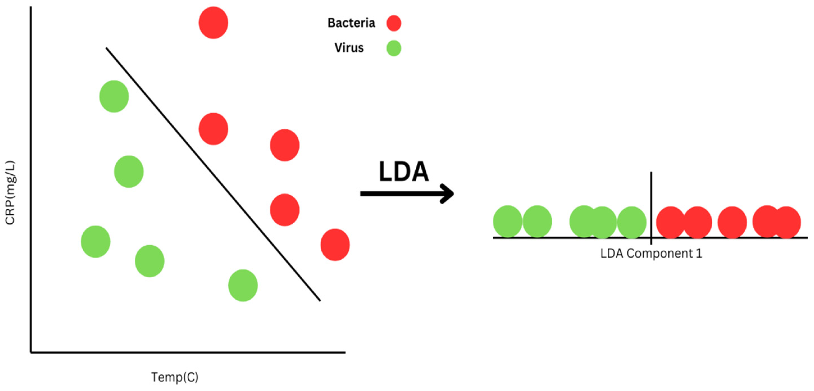
3.1.2. Linear Discriminant Analysis (LDA)

Linear discriminant analysis (LDA) helps us identify key features that differentiate different classes of objects or events. Discriminant function analysis is sometimes referred to as normal discriminant analysis. It can serve a dual purpose by classifying data and minimizing its dimensionality [50]. LDA acts like PCA, as both aim to find the integration of features that elucidate the input information. However, LDA considers the distinctions between data classes, whereas PCA does not consider any class differences [51].

Linear discriminant analysis (LDA) employs within- and between-class scatter to determine how well classes can be separated, as shown in Figure 1. Within-class scatter measures the spread or variability within each class, while between-class scatter measures the distance between the different classes. The objective is to discover a method to enhance class separation and minimize the spread within each class. It is represented as follows:

$$S_w=\sum _j{p}_j\times \left(co{v}_j\right)$$

(1)

where $p_j$ is the a priori probability of given class j and $co{v}_j$ is the covariance of given class j. The equation below is used to calculate a covariance matrix:

$$co{v}_j=\left(x_j-{\mu }_j\right){\left(x_j-{\mu }_j\right)}^T$$

(2)

Here, ${\mu }_j$ refers to the mean of given class j and $x_j$ refers to the vector of data points. The class of each scatter group is computed using the following equation:

$$S_b=\sum _j\left({\mu }_j-\mu \right){\left({\mu }_j-\mu \right)}^T$$

(3)

In this equation, $\mu$ represents the mean of that whole dataset, and the ratio of $S_b$ and $S_w$ is the optimizing criterion for LDA. The solution is obtained by maximizing the criterion. Each class in LDA with L-classes requires its own separate optimizing criterion. The optimizing components of every dependent type are calculated as

$$criterio{n}_j=inv\left(co{v}_j\right)\times S_b$$

(4)

where $inv\left(co{v}_j\right)$ represents matrix inverse of $co{v}_j$. The optimizing components of class-independent type are calculated as

$$criterion=inv\left(S_w\right)\times S_b$$

(5)

where $inv\left(S_w\right)$ represents matrix inverse of $S_w$.

In LDA, we transform original data by multiplying it with a transformation matrix for classification. The transformation matrix in LDA is defined as an eigen matrix of different criteria defined earlier. For any L-class problem, we would always have L-1 non-zero eigenvalues. We will only consider eigenvectors for which eigenvalues are non-zero.

For class-dependent LDA,

$$transforme{d}_j=transfor{m}_j^T\times se{t}_j$$

(6)

where $transforme{d}_j$ represents transformed dataset for jth class, $transfor{m}_j$ is the transformation matrix as described earlier containing eigenvectors and $se{t}_j$ is the set of data points of jth class.

For class-independent LDA,

$$transforme{d}_j=transform\_spe{c}^T\times data\_se{t}^T$$

(7)

where $transform\_spec$ is class-specific transformation, and $data\_set$ is the original dataset. Data points are classified utilizing either Euclidean distance or RMS distance after transforming, and the means are calculated for transformed data for every class. For a test vector, one should calculate the length from the test vector to all the means and then select the mean having the least distance from the test vector and assign the class of the mean to the test vector. Linear discriminant analysis (LDA) has various applications, including its adoption to identify antibiotic-resistant bacteria through surface-enhanced Raman spectroscopy [52,53]. It is also employed for classification tasks utilizing Raman spectroscopy data [54,55,56]. Additionally, LDA is used as a dimensionality reduction technique.

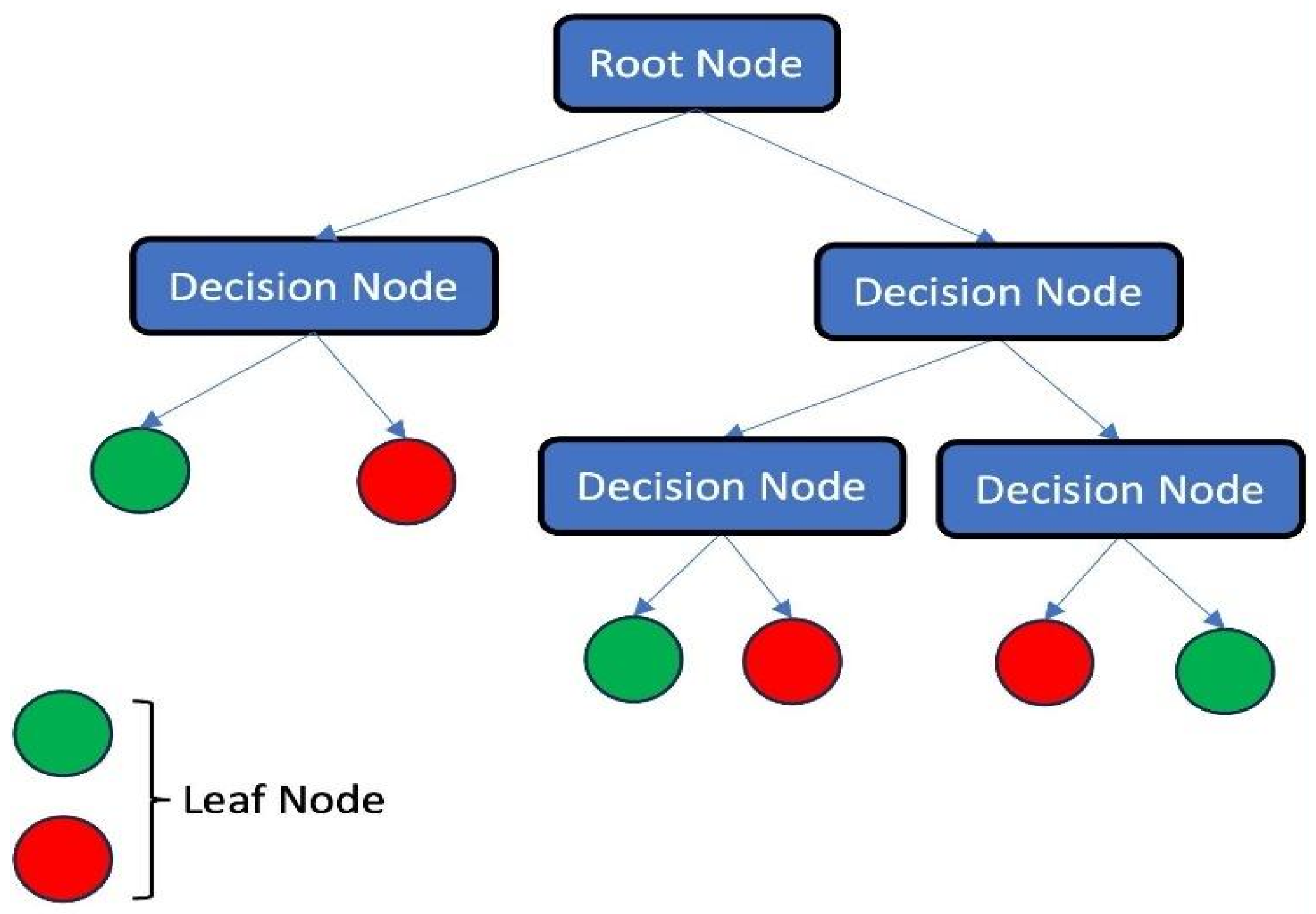
3.1.3. Decision Tree (DT)

Decision trees (DTs) are models that are useful for regression and classification tasks. When the target variable takes categorical values, it is referred to as a classification tree, and a regression type of decision tree algorithm is used when the target variable is continuous. In a classification tree, the leaves denote distinct classes, while the branches denote various combinations of features. Nodes contain groups of data points; at each branch, these data points are split into child nodes. A node is considered pure if all its data points belong to the same class, as shown in Figure 2. Various metrics are used to measure the purity of a node. Some of them are presented below.

• Entropy:

$$Entropy=\sum _i(-p_i\times lo{g}_2\left(p_i\right))$$

(8)

The higher the entropy value, the higher is the impurity in the node.

• Gini Index:

$$GiniIndex=1-\sum _i{p}_i^2$$

(9)

The higher the Gini index value, the higher the impurity in the node.

• Variance:

$$Variance={\displaystyle \frac{{\sum }_i{\left(x_i-\mu \right)}^2}{N}}$$

(10)

Entropy and the Gini index are used when the target variable is categorical, whereas variance is used when the target variable can take values from a range or continuous variable. An impure node is divided into smaller and purer nodes. This is called splitting of nodes. There may be several ways to split a node, but the split with the lowest value of entropy, Gini index, variance, or any other metric should be chosen. The gain in purity value after splitting a node is called information gain. It helps in feature selection for further tree construction.

$$Gain\left(S,f\right)=E\left(S\right)-\sum E\left(S_v\right){\displaystyle \frac{\left|S_v\right|}{\left|S\right|}}$$

(11)

Splitting stops when a desired purity level is achieved or based on other stopping criteria used according to the particular use case [57]. Decision trees (DTs) have a range of applications, such as classifying 12 common clinical pathogens using spectroscopy data [58]. They are also widely used for identification tasks, especially with SERS data [59]. Additionally, decision trees are employed in regression analyses to create decision trees for identifying pathogens in outbreaks of bovine respiratory disease derived from circumstantial factors [60].

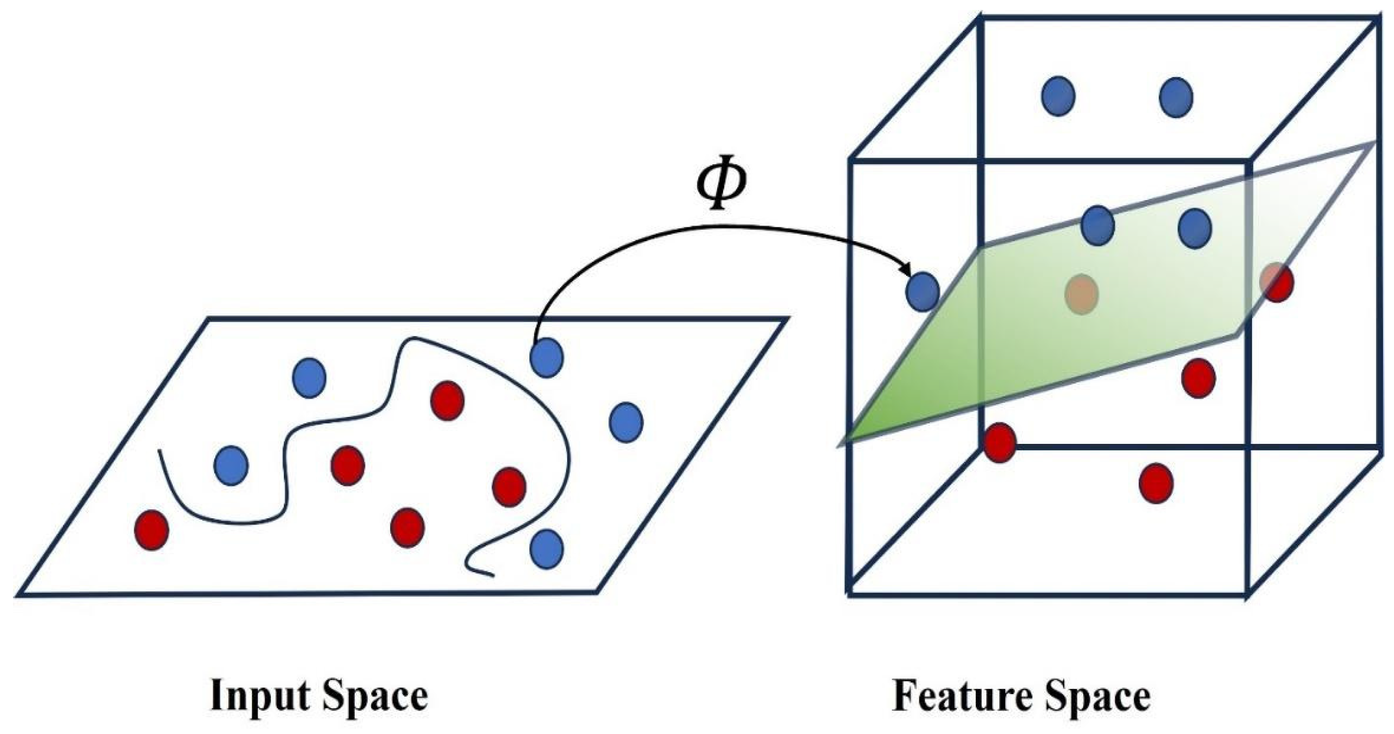
3.1.4. Support Vector Machines (SVMs)

The purpose of using an SVM is to classify spectral data between two groups, for example, to distinguish between resistant and susceptible bacterial strains. They construct hyperplanes that maximize the margin between different classes, improving classification accuracy, as shown in Figure 3.

Support vector machines (SVMs), or support vector networks, are applicable for both regression and classification problems. They work via constructing hyperplanes separating data into different classes. A hyperplane can be represented in general form using a vector w and a scalar b:

$$w^T·x+b=0$$

(12)

Let $y_i$ be target class label for a $x_i$ data point. As we are considering a two-class problem, we can safely assume that $y_i\in \{-1,+1\}.$ Any hyperplane that satisfies the following condition is considered a solution to the classification problem:

$$y_i\left(x_i ·w+b\right)\ge 1 \forall i$$

(13)

The margin for a hyperplane is a measure of the space between the provided hyperplane and the closed data point. Higher-margin hyperplanes are considered better for separating classes than the ones with low margins, as this reduces error. SVMs aim to identify a hyperplane that maximizes the margin for separating two classes. After applying some mathematical derivation, we get the following quadratic optimization problem:

• Minimize

  $$W\left(\alpha \right)=-{\alpha }^T·1+{\displaystyle \frac{1}{2}}{\alpha }^{T}H\alpha$$

  (14)
• Subject to

  $${\alpha }^{T}y=0$$

  $$\mathrm{And}, 0 \le \alpha \le C·1$$

  where there are l data points, $\alpha$ is a vector of l Lagrange multipliers, C is a constant, and $H$ is defined as follows:

  $$matrix{\left(H\right)}_{ij}=y_i{y}_j\left(x_i{·x}_j\right)$$

  (15)

  where $x_i$ is the ith data point with a dimensional vector. In this way, by solving the above minimization, we will have the value of $\alpha$. In addition, from the derivation of these equations, the equation of optimal hyperplane can be written as

  $$w=\sum _i{\alpha }_i{y}_i{x}_i$$

  (16)

One can reach the optimal hyperplane using the above equations and some steps. This type of SVM is called hard SVM, as it uses straight hyperplanes to classify data points. In real-world scenarios, we encounter situations where we need curved hyperplanes. Ignoring some data points close to the hyperplane is better for making curved situations more efficient. This is achieved by using a slack variable. Then, the updated equation for the feasibility of hyperplanes will be

$$y_i\left(w^T·x_i+b\right)\ge 1-S_k\forall i$$

(17)

The slack variable, denoted as $S_k$, allows a data point to be situated at a distance of $S_k$ on the side of the hyperplane that is not preferred or desired without causing a violation of the constraint. Similarly, the objective also changes accordingly. It can be minimized using

$$W\left(\alpha \right)={\displaystyle \frac{1}{2}}{w}^T·w-\sum {\lambda }_k\left(y_k\left(w^T·x_k+b\right)+S_k-1\right)+\alpha \sum S_k$$

(18)

The type of SVM where we allow slack variables is called soft-margin SVM. In the real world, there are problems which cannot be solved using simple linear SVMs. To solve such a problem, we allow non-linear decision boundaries and hyperplanes. To do that, we transform the original data using some function. This transformation involves mapping low-dimensional data to high-dimensional data, and this mapping is called a function. These functions are called kernel functions. Some standard kernel functions are described below.

Polynomial:

$$K\left(x,x^{\prime }\right)=<x,x^{\prime }{>}^d$$

(19)

$$\mathit{Or}, K\left(x,x^{\prime }\right)={\left(<x,x^{\prime }>+1\right)}^d$$

(20)

The second formulation helps in avoiding zero values in calculations for solving SVMs.

• Gaussian Radial Basis:

  $$K\left(x,x^{\prime }\right)=exp\left(-{\displaystyle \frac{{\left|\left|x-x^{\prime }\right|\right|}^2}{{\sigma }^2}}\right)$$

  (21)
• Exponential Radial Basis:

  $$K\left(x,x^{\prime }\right)=exp\left(-{\displaystyle \frac{\left|\left|x-x^{\prime }\right|\right|}{{\sigma }^2}}\right)$$

  (22)
• Multi-layer Perceptron:

  $$K\left(x,x^{\prime }\right)=tanh\left(\rho \left(x,x^{\prime }\right)+e\right)$$

  (23)

In addition to their use in classification tasks, support vector machines (SVMs) can be utilized for regression tasks by incorporating alternative loss functions. These regression models are both linear and non-linear. Linear regression models commonly employ loss functions such as e-intensive, quadratic, and Huber [61]. Support vector machines (SVMs) are used in various applications, particularly spectroscopy. For instance, SVMs were adopted to differentiate drug (antibiotic) resistant strains with the application of surface-enhanced Raman spectroscopy and to classify multiple clinical pathogens with Raman spectroscopy data [62,63]. Furthermore, SVM classifiers have been utilized to identify the existence of concentration levels of antibiotics using absorption spectra obtained from raw milk using machine learning implementation to the spectra of a nano biosensor [64]. Another study utilized a HTMI (hyperspectral transmission microscopic imaging) system for the ultra-high-speed recognition and classification of the mixture of pathogenic bacteria at the single-bacterium level via PCA and SVM [62]. Similarly, another study showed the rapid determination of infection due to Mycobacterium tuberculosis and its resistance through the machine learning analysis of SERS fingerprinting spectra for classification tasks using Raman spectroscopy data to classify mixed bacteria using hyperspectral transmission microscopic imaging [63].

3.1.5. Random Forests

Random forests consist of multiple decision trees that improve classification performance by averaging the predictions of multiple trees, as shown in Figure 4. They are effective in handling large datasets and complex patterns in spectroscopic data. The random forest (RF) algorithm is widely implemented during classification and regression tasks. The RF method utilizes numerous decision trees to enhance the accuracy of its given predictions.

Unlike a single decision tree, which can easily overfit the data, RF’s ensemble method helps to mitigate overfitting and enhance generalization by aggregating the predictions of multiple trees, leading to more adaptable and precise outcomes. Every decision tree within a random forest is trained with the help of a randomly selected fraction of the provided input original dataset. Also, each provided decision tree is trained on a subset of extracted features. This helps avoid overfitting in training any single decision tree of the RF and makes it more robust. RF models predict outputs using majority voting among the decision trees. In the case of classification, RFs take the output label from all decision trees and output the label given by the most trees. In the application of regression, the provided output is just an average of values given by individual trees [65].

3.1.6. Logistic Regression (LR)

Logistic regression is a mathematical approach to address categorization problems, especially those with two distinct classes. When LR utilizes the given sigmoid ($\sigma$) function, then

$$\sigma \left(z\right)={\displaystyle \frac{1}{1+e^{-z}}}$$

(24)

which changes the numerical values found after multiplying features with weights into probabilities of individual classes. z is equal to the following equation:

$$z=X· w+b$$

(25)

where X is the feature matrix (rows are data points and columns are values of features), w is the weights vector, and b is a coefficient vector. So, the final equation of the probability of a class in logistic regression will be

$$p\left(X:b,w\right)={\displaystyle \frac{1}{1+e^{-\left(X·w+b\right)}}}$$

(26)

Usually, two classes are denoted as 1 and 0. So, for class = 1, the probability is $p\left(X:b, w\right) = p\left(x\right)$, whereas for class = 0, the probability is $\left(1-p\left(x\right)\right)$. Then, we use a mathematical technique called likelihood maximization on the equation to find the weight vector in the equation. The likelihood function for logistic regression is

$$L\left(b, w\right) =\prod _{i=1}^{n}p{\left(x_i\right)}^{y_i}{\left(1-p\left(x_i\right)\right)}^{1-y_i}$$

(27)

In the above equation, n denotes the total number of points present in the used dataset. Taking natural log on both sides and differentiating to maximize likelihood, we get the following equation:

$${\displaystyle \frac{\partial log\left(L\left(b,w\right)\right)}{\partial w_j}}=\sum _{i=n}^n\left(y_i-p\left(x_i:b,w\right)\right)x_{ij}$$

(28)

When solving the differential equation, we will get weight and coefficient vectors. These are further used to predict each class’s probability using the earlier probability equation, which is further extended for K classes by replacing the sigmoid function with the softmax function, as follows:

$$softmax\left(z_i\right)={\displaystyle \frac{e^{z_i}}{{\sum }_{j=1}^K{e}^{z_j}}}$$

(29)

where $z_i=X_i·w_i+b_i$. $z_i$ is the ith value of z vector and the length of z vector is equal to K. And following a similar procedure as for the two classes, we get the probability for class c as

$$P\left(Y=c|\overrightarrow{X}=x\right)={\displaystyle \frac{e^{x·w_c+b_c}}{{\sum }_{k=1}^K{e}^{x·w_k+b_k}}}$$

(30)

In cases where two or more classes are involved, the output is decided by calculating the probability for all classes and then choosing the class with the maximum probability [66]. Logistic regression is widely used for classification tasks. One notable application is in the classification of data obtained from Raman spectroscopy. This method effectively distinguishes between different categories based on spectral data [67]. One study demonstrates the classification capability of logistic regression on SERS data of miRNAs, showing its utility in distinguishing between various miRNA types related to pancreatic cancer [68].

3.1.7. Gradient Boosting (GB)

Gradient Boosting (GB) is an immensely effective ensemble algorithm within supervised machine learning that serves the purpose of both classification and regression tasks. It sequentially builds models such that every new model tries to eliminate errors made by previous models, as shown in Figure 5. This algorithm combines several base learners, typically decision trees.

The algorithm begins by training a base learner and then identifying data points that the base learner incorrectly classifies. Each base learner is trained using these data points as the training set. This process is continued for the entire ensemble. The incorrect data points in each step are called residual errors or Shrinkage, also known as the learning rate $(\eta$), which is used to update the ensemble using the weights of the newly trained base learner represented by

$$F_m\left(x\right)=F_{m-1}\left(x\right)+\eta ·h_m\left(x\right)$$

(31)

where $F_m\left(x\right)$ is the updated model after m iterations, $F_{m-1}\left(x\right)$ is the model after m-1 iterations, $h_m\left(x\right)$ is the desired prediction of the mth weak learner, and $\eta$ is the learning rate [69].

3.1.8. AdaBoost

AdaBoost, short for adaptive boosting, is a supervised ensemble method for classification and regression problems. AdaBoost also builds several weak learners (decision tree stumps of a single depth) sequentially, with every new learner trying to eliminate errors made by previous models [70], as shown in Figure 6.

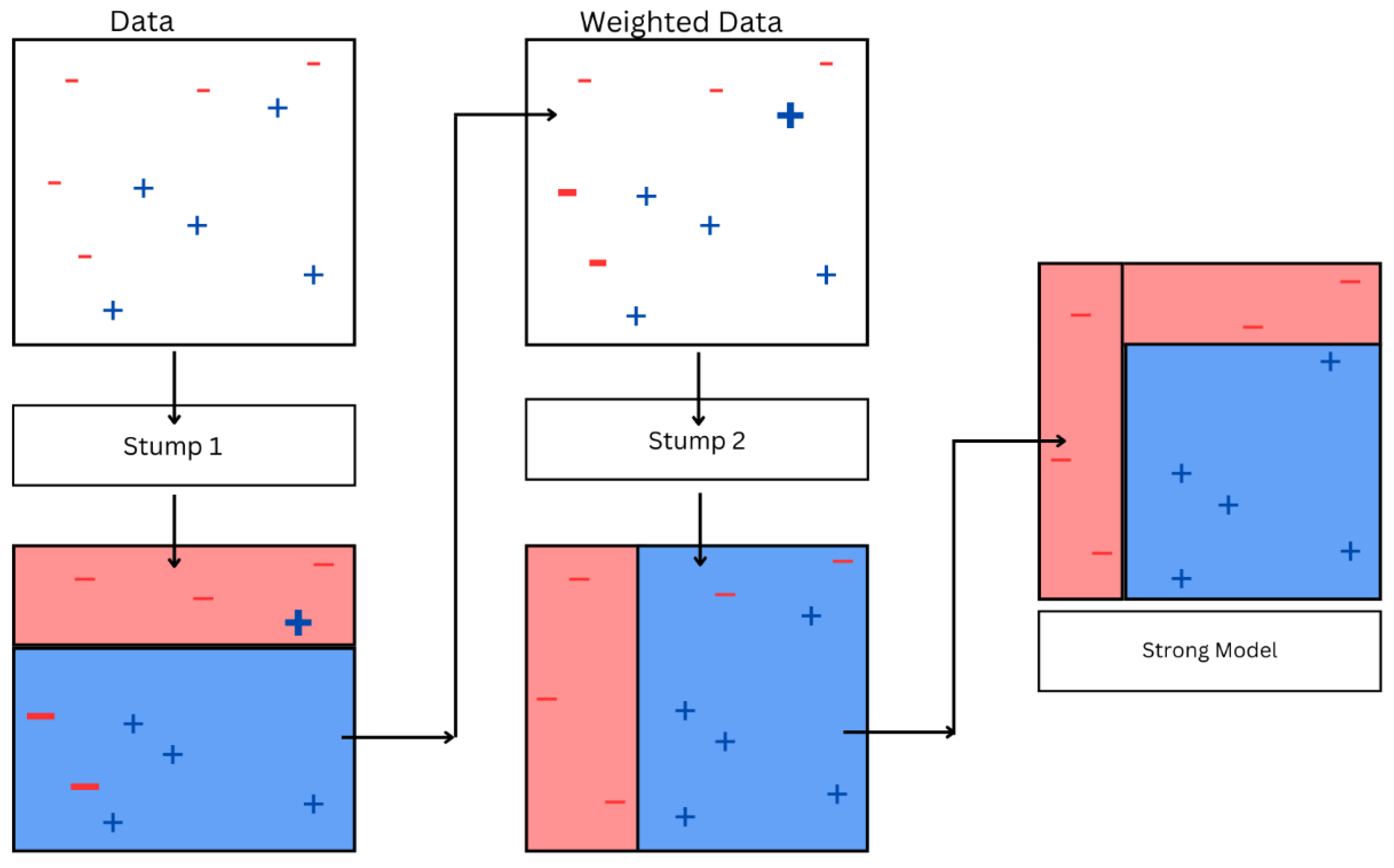
The following are the steps for AdaBoost:

(a)

Initialize equal weights for each data point. For example, if there are N data points, then each data point is assigned ${\displaystyle \frac{1}{N}}$ weight.

(b)

A weak classifier is trained on these weighted data points. The classifier tries to minimize weighted error, where the error for each incorrect prediction is weighted by the weight of the data point for which the prediction was made.

(c)

The learner’s error rate, ϵ, is determined by evaluating the weighted sum of incorrectly predicted samples. This error rate indicates how effectively the learner performs on the weighted data.

(d)

Calculate the weight of $\alpha$ by using

$$\alpha ={\displaystyle \frac{1}{2}}ln\left({\displaystyle \frac{1-ϵ}{ϵ}}\right)$$

(32)

(e)

This weight signifies the participation of this learner in the end prediction of the ensemble. Better-performing learners will have a higher weight, representing a higher contribution in the final prediction.

Update the weights of the data points using the following formula:

$$w_i\leftarrow w_i·e^{\alpha ·y_i·h\left(x_i\right)}$$

(33)

where $w_i$ is the weight of ith sample, $y_i$ is the true label, and $h\left(x_i\right)$ is the prediction of the weak learner, followed by normalizing the weights of the data points to ensure that they add up to one, ensuring fairness for the data points in the next iteration. Repeat the steps until the specified number of iterations or certain criteria are satisfied. In this process, each iteration introduces a new weak learner to the model ensemble.

(f)

The end model is constructed by summing the outputs of multiple weak learners using the calculated weights. When the model is used for predicting the label of a new sample, each weak classifier contributes to the prediction with a weight, and the ultimate prediction is calculated by taking a weighted mean of the estimates made by each and every weak classifier.

Adaboost is extensively used to enhance classification performance. One notable application is its use in classifying data obtained from spectroscopy data by boosting the accuracy of weak classifiers, where Adaboost effectively improves the differentiation between categories based on spectral data [71,72].

3.1.9. Neural Networks

Feature extraction and classification in spectral imaging data are achieved using convolutional neural networks (CNNs) and recurrent neural networks (RNNs). The implementation of CNNs has proven exceptionally valuable for analyzing spatial patterns in spectroscopic images. Neural networks are categorized as a part of algorithms in machine learning that are developed by inspiration from the human brain. They consist of neurons similar to the human brain, known as interconnected layers of nodes (or neurons). They can be supervised or unsupervised, depending on the application. Three main types of neural network layers are distinguished: input, hidden, and output. The input layer is responsible for receiving the input data, with k neurons representing individual features of the data. The hidden layer transforms the input passed from the input layer through connections and activation functions. Neurons in hidden layers are interconnected, and each connection has some weight associated with it. When data is sent from one neuron to another, it is transformed by multiplying it by the associated weight and then applying an activation function. The end or output layer of a neural network’s corresponding quantity of neurons is determined by the number of possible outputs that the network can provide to produce the final output.

The training of neural networks is very crucial. One should minimize the inconsistency between the predicted and actual outcomes by iteratively adjusting the weights within the network. In neural networks, the term “loss” means the divergence between the actual result and the anticipated output, which is quantified by a loss function. Another important term is “backpropagation,” where the network adjusts its weights by reversing the flow of loss through the system, which is employed by optimization algorithms like gradient descent. The following are a few commonly used loss functions in neural networks:

(a)

Mean Squared Error Loss Function:

$$Loss\left(y,\widehat{y}\right)={\displaystyle \frac{1}{N}}\sum _{i=0}^N{\left(y_i-{\widehat{y}}_i\right)}^2$$

(34)

(b)

Cross Entropy Loss Function:

$$Loss\left(y,\widehat{y}\right)=-\sum _{i=0}^N{\widehat{y}}_i·log\left(y_i\right)$$

(35)

(c)

Mean Absolute Percentage Error/Deviation:

$$Loss\left(y,\widehat{y}\right)={\displaystyle \frac{100\%}{N}}\sum _{i=0}^N{\displaystyle \frac{\left|y_i-{\widehat{y}}_i\right|}{{\widehat{y}}_i}}$$

(36)

where the value of y represents the actual result, $\widehat{y}$ represents the anticipated value, and N explains the quantity of features in the data for continuous values. One of the major key components is an “activation function,” which ensures learning and understanding of complex relationships in the network. The following are a few examples of commonly utilized activation functions:

(a)

Binary step function:

$$f\left(x\right)=\left\{\begin{array}{c}0, x<0\\ 1, x\ge 0\end{array}\right.$$

(37)

(b)

Linear activation function:

$$f\left(x\right)=x$$

(38)

(c)

Sigmoid/logistic function:

$$f\left(x\right)={\displaystyle \frac{1}{1+e^{-x}}}$$

(39)

(d)

Tanh function:

$$f\left(x\right)={\displaystyle \frac{\left(e^x-e^{-x}\right)}{\left(e^x+e^{-x}\right)}}$$

(40)

(e)

Rectified Linear Unit, popularly known as ReLU function:

$$f\left(x\right)=max\left(0,x\right)$$

(41)

(f)

Leaky Rectified Linear Unit function (Leaky ReLU):

$$f\left(x\right)=max\left(0.1x,x\right)$$

(42)

(g)

Parametric ReLU function:

$$f\left(\alpha ,x\right)=max\left(\alpha x,x\right)$$

(43)

(h)

Exponential Linear Unit (ELU) function:

$$f\left(\alpha ,x\right)=\left\{\begin{array}{r}\alpha \left(e^x-1\right), x<0\\ x, x\ge 0\end{array}\right.$$

(44)

(i)

Softmax function:

$$f\left(x_i\right)={\displaystyle \frac{e^{x_i}}{{\sum }_{j=1}^n{e}^{x_j}}}$$

(45)

where n defines the quantity of neurons in the output layer used.

(j)

Swish function:

$$f\left(x\right)={\displaystyle \frac{x}{1+e^{-x}}}=x\ast sigmoid\left(x\right)$$

(46)

(k)

Gaussian Error Linear Unit (GELU) function:

$$f\left(x\right) = 0.5x\left(1+tanh\left[\sqrt{\left({\displaystyle \frac{2}{\pi }}\right)}\left(x + 0.044715x^3\right)\right]\right)=xP\left(X\le x\right)$$

(47)

where $P\left(X\le x\right)=\Phi \left(x\right)$ is used for symbolizing the cumulative probability curve of the standard normal distribution.

(l)

Scaled Exponential Linear Unit, also called SELU function:

$$f\left(\alpha ,x\right)=\lambda \left\{\begin{array}{r}\alpha \left(e^x-1\right), x<0\\ x, x\ge 0\end{array}\right.$$

(48)

There are numerous neural networks that have been developed over time, and each of them has different purposes or applications and is used based on the problem requirement. An example is a feedforward neural network, which is also known as a multilayer perceptron (MLP). It allows data to move in one direction, from input to output, without loops, making it straightforward and widely used for handling complex patterns. On the other hand, convolutional neural networks (CNNs) are designed to process mesh-like network inputs such as surface images and pictures utilizing convolutional layers to learn hierarchical feature representations, making them suitable for image analysis. Similarly, recurrent neural networks (RNNs) work well for sequential inputs like time series or text by learning to capture temporal dependencies, making them suitable for language prediction and forecasting. There are a few variants in RNN, which include Gated Recurrent Units (GRUs) with Long Short-Term Memory (LSTM) networks and Generative Adversarial Networks (GANs). LSTMs are adept at managing long-term dependencies within data, and GANs include a pair of interconnected networks or a generator to generate new data samples to verify the authenticity of these generated samples by using a discriminator. Another type of unsupervised neural network is Autoencoders, which learn compressed representations of initial variables by compressing and transforming them into a lower-dimensional space and reorganizing the original data input.

Neural networks are extensively utilized across diverse fields for numerous purposes. Convolutional neural networks (CNNs) are employed for classification using spectroscopy data and to classify resistance in TB-causing bacterial strains [73]. Long Short-Term Memory Networks (LSTMs) have been used to classify Staphylococcus species using surface-enhanced Raman spectroscopy data [71]. A combination of CNN, LSTM, MLP (multilayer perceptron), GRU (Gated Recurrent Unit), and RNN (recurrent neural networks) was utilized to classify clinically important pathogens using surface-enhanced Raman spectroscopy [74]. CNN, GRU, LSTM, and MLP were also applied to quickly identify whether a person is infected with Mycobacterium tuberculosis and determine their drug resistance status using Raman spectroscopy [63]. MLPs and CNNs have also been used to classify Candida species using Raman spectroscopy [75]. Based on Raman spectroscopy signals, the deep neural network algorithm is employed to predict the growth status of an unknown bacteria strain, which is composed of a single hidden layer with eight neurons employing Rectified Linear Unit (ReLU) activation function connected with the hidden layer and associated with a sigmoid activation function in the output layer. Lastly, using Raman spectroscopy, MLPs were used to identify urinary tract infection bacteria [76]. In

Table 3. Summary of major useful supervised learning algorithms and their application in antibiotic resistance studies.

Method	Description	Applications in Antimicrobial Resistance
PLS	A linear regression model that transforms predictors and responses into a new domain. Useful when the target variable is continuous or categorical.	Raman spectroscopy coupled with PLSR successfully identified Campylobacter species in mixed samples of C. jejuni, E. coli, C. upsaliensis, and C. fetus [77].
LDA	Projects data to a lower-dimensional space for class separation, enhancing interpretability.	PCA-LDA models combined with IR spectroscopy differentiated between resistant and sensitive E. coli strains [78]. Also applied to SERS data to classify clinical pathogens [52].
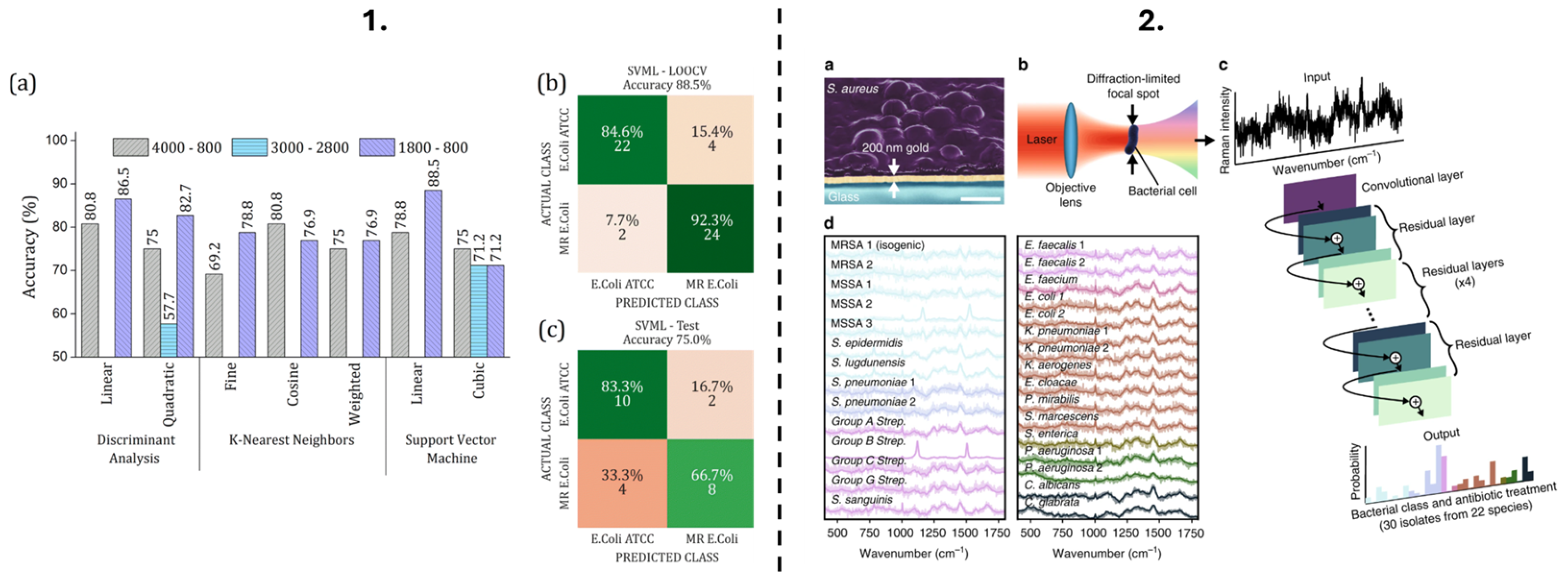
SVM	Projects data into a higher-dimensional space and creates hyperplanes for classification.	SVM with Raman spectra enabled accurate identification of infectious fungi with 100% sensitivity and specificity using single-cell Raman spectroscopy (SCRS) [75].
RF	An ensemble of decision trees trained on different dataset subsets and features. Provides robust classification and handles overfitting well.	Combined with spectroscopy for classification of antibiotic-resistant bacterial strains; improved feature importance interpretation [79].
Logistic Regression	Uses a sigmoid function to predict categorical outcomes; particularly effective in binary classification problems.	Used as a baseline classifier in AMR studies; interpretable and efficient in small-scale Raman datasets [80].
AdaBoost	Similar to GB but increases weight for misclassified points. Focuses learners on difficult cases to improve accuracy.	Boosts weak classifiers on spectroscopy datasets; useful in settings with class imbalance.
Neural Network	Inspired by the human brain; consists of interconnected layers for learning non-linear patterns. Supports classification and regression tasks.	Neural networks, including ANN and CNN, were used for bacterial and fungal infection classification from Raman and IR databases with >90% accuracy [12,81]. CNNs also identified MRSA vs. MSSA with 89% accuracy [12].
U-Net (CNN architecture)	Specialized CNN architecture for image-like data; ideal for segmentation and feature extraction.	U-Net architecture achieved high accuracy in classifying antibiotic resistance from Raman spectra of 30 bacterial and yeast isolates [82].

, we have highlighted a few significant studies that were used for the rapid identification of bacteria and their antibiotic resistance using machine learning and spectroscopy.

3.2. Unsupervised Learning

Unsupervised learning algorithms are employed to detect and analyze patterns in data without relying on predefined labels. Unlike supervised learning, they do not require input–output pairs. Instead, they explore the data to find hidden structures or patterns on their own. They are useful for exploring the underlying structure of spectroscopic data and identifying clusters of similar bacterial strains. Unsupervised learning encompasses clustering, dimensionality reduction, and association, as shown in Figure 7. Clustering groups data points based on similarities and is used for identifying different cell types in single-cell RNA sequencing data, grouping protein structures, or clustering bacterial species based on genetic information, using algorithms like K-Means, hierarchical clustering, and DBSCAN.

Dimensionality reduction methods, such as principal component analysis (PCA), t-distributed Stochastic Neighbor Embedding (t-SNE), and linear discriminant analysis (LDA), are introduced to reduce the number of useful features in a dataset while retaining useful information. These methods are particularly employed during visualizing high-dimensional genomic data, reducing noise in biological signal data, and extracting important features from complex datasets [83]. Association techniques, like Apriori, Eclat, and FP-Growth, help discover relationships between variables, such as finding associations between genetic markers and diseases, identifying frequently co-occurring mutations in cancer cells, and analyzing metabolic pathways.

3.2.1. Principal Component Analysis (PCA)

PCA is a frequently utilized approach in spectral data analysis for minimizing the dimensionality of the data. This is operated by converting the initial high-dimensional input data into a lower-dimensional space referred to as the principal components. Using spectral fingerprints, PCA can efficiently differentiate groups of bacterial strains [84]. Here, the matrix Y of dimensions N × K stores I observations with K dependent variables. X with dimensions N × M stores the inputs of M estimated values compiled for I observations. To decompose matrix X, the decomposition of its single value is utilized.

$$X=S\Delta V^T$$

(49)

where

$$S^{T}S=V^{T}V=I$$

(50)

The left and right singular vectors are stored in S and V matrices, respectively. Each singular values are positioned as elements that lie on the diagonal within the matrix ∆. The identity matrix I is used to express the matrices S, V, and ∆ in a specific way. The singular vectors are arranged parallel to the unit values. Those are directly proportional to the square root of each of the element’s variances present inside the matrix. The singular vectors on the left, found in the columns in matrix S, are subsequently utilized in standard regression to predict Y [85].

3.2.2. Hierarchical Cluster Analysis (HCA)

Hierarchical cluster analysis organizes similar data points into clusters, which are applied to gain meaningful information about the connections between bacterial strains and their resistance patterns. This technique can be broadly classified into two types: agglomerative clustering (called bottom-up), where clusters are progressively merged, and divisive clustering (called top-down), where clusters are progressively divided. One of the studies by Berrazeg et al. demonstrated the use of hierarchical clustering to monitor antibiotic resistance phenotypes in Klebsiella pneumoniae strains, showing its effectiveness in identifying and organizing resistance patterns [86]. The primary goal of agglomerative clustering is to make a single large cluster by assuming that each data point initially represents an individual cluster. That is why it is also called the bottom-up clustering technique. The basic algorithm for agglomerative clustering involves several steps: the first step is to treat every data point as a separate group, followed by the calculation of a proximity matrix to measure the similarity or distance between different clusters. The two nearest clusters in the proximity matrix are then merged into a larger cluster. This process is repeated continuously, re-computing the proximity matrix and merging the closest clusters at every step until only a single cluster remains [87]. However, divisive clustering is a top-down clustering technique that begins with a single cluster containing all the data points which progressively splits this large cluster into smaller clusters, with each iteration creating new clusters that contain fewer data points. This approach is the opposite of agglomerative clustering, which starts with individual data point clusters and gradually combines them into larger clusters. The initial step in divisive clustering involves creating a single cluster encompassing all the data points. This large cluster is then divided using a flat-clustering technique like K-means. This next stage identifies the cluster with the highest Sum of Squared Error (SSE) and further splits it, and the process continues until a defined stopping criterion is met, such as reaching a specified number of clusters or achieving optimal intra-cluster similarity. The proximity between two clusters is calculated using different metrics, each with its own merits. A few of the primary metrics are described below.

MIN: In this metric, the resemblance between the two clusters C₁ and C₂ is determined by calculating the lowest similarity value among pairs of data points, where one point P_i belongs to C₁ and the other point P_j belongs to C₂. This methodology is likewise known as the single-linkage algorithm.

$$Sim\left(C_1,C_2\right)=Min Sim\left(P_i,P_j\right) such that P_i\in C_1 and P_j\in C_2$$

(51)

This MIN approach for clustering offers advantages, such as its ability to separate clusters with irregular or non-elliptical shapes, as it does not assume any specific geometric form and is useful for handling complex patterns. It is also effective when there is a significant gap between clusters; it helps accurately identify and separate them into distinct clusters. The drawback of this approach is that, sometimes, it fails to handle noise between clusters when significant noise or overlapping data points affect the minimum similarity measure, resulting in incorrect cluster assignments. These pros and cons should be carefully considered when applying the MIN approach for cluster analysis.

MAX: This metric determines the resemblance between two groups, C₁ and C₂, by calculating the highest resemblance between any two data points, as P_i belongs to C₁ whereas P_j belongs to C_2, and maximum similarity values are used to evaluate the similarity between clusters.

$$Sim\left(C_1,C_2\right)=Max Sim\left(P_i,P_j\right) such that P_i\in C_1 and P_j\in C_2$$

(52)

The approach effectively deals with noise between clusters by focusing on finding the maximum similarity between data points in different clusters. Therefore, the MAX approach is useful for accurately identifying and separating clusters even in the presence of noise. One of the drawbacks of this method is that it fails to identify clusters with irregular shapes.

Group Average: This metric evaluates the similarities between all pairs of points and finds the average similarity. Those points can be evaluated for similarity by utilizing distance metrics such as Euclidean distance or Manhattan distance, etc. In mathematical terms, it can be expressed as

$$Sim\left(C_1,C_2\right)={\displaystyle \frac{\sum Sim\left(P_i,P_j\right)}{\left|C_1\right|\ast \left|C_2\right|}}$$

(53)

In this equation, $P_i\in C_1 \& P_j\in C_2$.

One advantage of the group average approach is its ability to effectively separate clusters in the presence of noise between them. One drawback of the group average approach is that it tends to favor globular clusters over other types of clusters.

Ward’s Method: This method is applicable for quantifying the resemblance between two groups like group average; Ward’s method computes the total squared intervals between P_i and P_j. In mathematical terms, it can be expressed as

$$Sim\left(C_1,C_2\right)={\displaystyle \frac{\sum {\left(Sim\left(P_i,P_j\right)\right)}^2}{\left|C_1\right|\ast \left|C_2\right|}}$$

(54)

Ward’s method is effective in separating clusters even in the presence of noise between them. However, it is known to have a bias towards detecting and forming globular clusters. Hierarchical clustering is represented visually by the dendrogram. The sequence of cluster merges or splits is represented in a dendrogram as a tree diagram.

3.2.3. K-Means Clustering

K-means clustering iteratively groups data points into distinct clusters without supervision, making it a machine-learning unsupervised algorithm. It divides into separate clusters that do not overlap with each other. The K-means algorithm initially selects k initial centroids from the dataset, which are used as the starting points for the clustering process. The selection could be random or manual. Once the centroids are selected, each data point is assigned to a centroid based on their distance to each centroid, using a distance metric. The centroid with the lowest distance value is assigned to each data point Some of the most widely used distance metrics are described below.

(a)

Euclidean distance:

$$d\left(p,q\right)=\sqrt{\sum _{i=1}^n{\left(q_i-p_i\right)}^2}$$

(55)

In the Equations (55) and (56), p and q are data points with n features; $p_i$ and $q_i$ represent the value of the ith feature of p and q, respectively.

(b)

Manhattan distance:

$$d\left(p,q\right)=\sum _{i=1}^n\left|p_i-q_i\right|$$

(56)

(c)

Mahalanobis distance:

$$d\left(p,q\right)=\left(p-q\right){\mathsf{\Sigma }}^{-1}{\left(p-q\right)}^T$$

(57)

In this equation, p and q are data points and $\mathsf{\Sigma }$ is the covariance matrix of the complete input data.

(d)

Hamming distance:

$$d\left(p,q\right)=\sum _{i=1}^n\left|p_i-q_i\right|$$

(58)

In this equation, p and q are data points with n features; $p_i$ and $q_i$ represent the the value of the ith feature of p and q, respectively. This distance is used for measuring differences in binary strings.

(e)

Cosine distance:

$$d\left(p,q\right)=1-{\displaystyle \frac{p·q}{{\left|\left|p\right|\right|}_2{\left|\left|q\right|\right|}_2}}$$

(59)

Once every data point is allocated to its centroids, each k cluster’s centroid is updated by finding the average of the data points in that cluster. The process continues until the centroids do not change any more. Clustering methods can be used to find groups within data by grouping similar data points. Clustering helps expose structures that are not initially transparent, facilitating insights and informed decision-making in various fields.

A few examples of unsupervised learning approaches applied in antibiotic resistance studies are summarized in

Table 4. Summary of major useful supervised learning algorithms and their application in antibiotic resistance study.

Method	Description	Applications in Antimicrobial Resistance
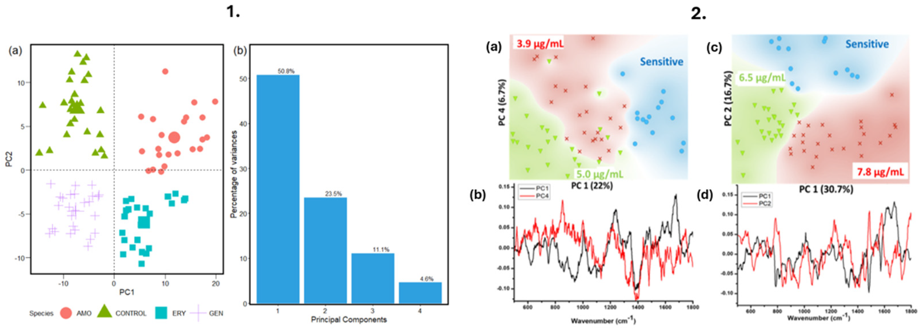
PCA	A dimensionality reduction technique widely used in spectroscopy to reduce features into principal components for easier visualization and interpretation.	Raman spectroscopy was used to find spectral differences between colistin-sensitive and resistant E. coli strains using PCA [88]. PCA and clustering were applied to identify similar spectral patterns among Mycobacterium bovis and Mycobacteriales strains [73].
HCA	Groups similar data points into clusters using a tree-like dendrogram, which helps identify relationships among observations.	Used in conjunction with Raman spectroscopy to classify bacterial strains and monitor structural similarities across resistant and non-resistant species [77].
K-Means Clustering	A centroid-based algorithm that partitions data into a predefined number of clusters based on distance metrics.	Applied in spectral data to differentiate microbial strains by their biochemical signatures, especially in unsupervised analysis settings [89].

.

3.3. Deep Learning

Deep learning can handle large and complex signals, specifically convolutional neural networks (CNNs) and recurrent neural networks (RNNs), which have offered significant promise in the differentiation of resistant and sensitive strains [12,52,58]. Convolutional neural networks (CNNs) are very good at analyzing spectroscopic images, finding important details, and sorting bacterial strains into categories. They have been used to analyze hyperspectral imaging data to identify resistant bacteria and automatically extract relevant features from primary data [90]. CNNs exclude the requirement of manual feature engineering. Algorithms such as recurrent neural networks (RNNs) and Long Short-Term Memory (LSTM) networks work best for assessing time-dependent monitoring, like bacterial growth and bacterial response to antibiotics. They capture temporal dependencies, making them helpful in modeling the dynamics of bacterial populations under antibiotic stress. They use ensemble learning techniques similar to Gradient Boosting and AdaBoost to enhance accuracy and stability by collective outlook from different models, leveraging the strengths of diverse models to create more stable and consistent predictions [91]. In the Gradient Boosting algorithm, models are built sequentially, where each new model is generated by correcting errors made by previous ones; therefore, Gradient Boosting is useful for classification tasks in antimicrobial resistance (AMR) research, utilizing spectroscopy data to improve detection accuracy [92]. On the other hand, AdaBoost adjusts the model weights by incorrectly classifying instances in each iteration, which enhances the performance of weak classifiers, making it effective for AMR detection using spectroscopic data.

3.4. Transfer Learning

Transfer learning becomes a valuable approach for AMR detection when labeled data is limited, as it leverages knowledge from pre-trained models on similar tasks to enhance performance on the target task [93]. Models that are already trained on large datasets like ImageNet can help improve specific AMR detection tasks. They require fewer labeled data and less speed for the development of new models. Additionally, domain adaptation techniques allow models trained on one domain, such as general bacterial classification, to perform well on a related domain, such as specific antibiotic resistance detection [94]. This helps machine learning models work well with different datasets and situations.

3.5. Reinforcement Learning (RL)

Reinforcement learning is a type of method which involves improving decision-making abilities through interaction with an environment and gaining responses in the form of incentives or consequences, also known as RL agents. Although RL is not widely applied in AMR research, it has great potential for optimizing treatment strategies and understanding bacterial adaptation to antibiotics. RL can be utilized to develop adaptive treatment strategies that minimize the emergence of resistance by simulating various treatment scenarios and allowing RL agents to learn optimal antibiotic usage patterns. RL models can be useful for studying the evolutionary dynamics of bacteria under different selective pressures, providing insights into bacterial adaptation to antimicrobial agents and informing the development of strategies to counteract resistance [95].

4. Case Studies and Applications of ML in AMR Research

Recent advancements have demonstrated the efficacy of integrating machine learning (ML) with spectroscopic methods for AMR research [12,82,90,96]. Many studies report that using FTIR spectroscopy combined with ML algorithms is promising in predicting antibiotic resistance, offering a faster and more precise alternative to traditional antibiotic susceptibility testing (AST) methods [25,26,28]. One study reported the use of FTIR spectroscopy data to accurately predict resistant and sensitive E. coli using various ML techniques [97]. Another published study proved that Raman spectroscopy combined with convolutional neural networks (CNNs) can identify different bacterial phenotypes precisely [12], as shown in Figure 8. This method achieved high accuracy in distinguishing antibiotic-resistant strains from susceptible ones, significantly improving pathogen identification speed and diagnostic outcomes in clinical settings. Automated AST systems using spectroscopic data and ML models streamline diagnostics, helping clinicians make informed treatment decisions quickly and reducing antibiotic misuse [98,99,100].

Many studies have used unsupervised dimension techniques to find antibiotic resistance. For example, PCA spatial patterns have been used to identify resistance profiles of various antibiotic-treated species by FTIR datasets from S. aureus species [101]. Another study utilized PCA for dimension reduction and identified between colistin-sensitive and -resistant E. coli strains using Raman spectra 81, as shown in Figure 9 [102].

The integration of quantitative PCR (qPCR) with ML techniques has enhanced the detection of AMR genes in bacterial populations [103]. ML improves the accuracy and speed of gene detection, supporting effective monitoring and management of antibiotic resistance in clinical settings. This approach facilitates the tracking of resistance gene spread and aids in implementing infection control measures. Moreover, near-infrared (NIR) spectroscopy combined with ML enables the real-time monitoring of bacterial responses to antibiotic treatment [47]. Yamaguchi et al. developed an NIR-II imaging platform and studied the real-time monitoring of infection by E. coli against the immune cells of mice in vivo [104].

Different spectroscopic techniques unified with ML algorithms have also shown great promise in terms of antibiotic resistance, which is unfolding in agriculture, as well as in various other environments [105,106]. Raman spectroscopy and FTIR have proven to be very practical and effective in detecting resistant bacteria that thrive in soil, water, or inside animals and help prevent further spread of resistance and infection. These highly efficient and non-invasive methods offer a deeper understanding of the overuse and misuse of antibiotics and the consequences of AMR. On top of that, public health services have also started implementing integrated ML–spectroscopic techniques for AMR monitoring. For example, Huang et al. tested domestic sewage and adult male urine samples to explore mixed antibiotic presence with the help of spectral ML [107]. Shams et al. researched the rapid detection of AMR in uropathogenic Escherichia coli (UPEC) by using optical photothermal infrared spectroscopy in their innovative study [108]. These approaches help public health teams in the fight against resistant infections, stopping them from spreading further by rapidly and accurately analyzing large sets of data.

5. Discussion and Future Directions

AMR is one of the most alarming global health threats of the 21st century, complicating the approach to the treatment of bacterial infections and thereby greatly raising the risk of morbidity, mortality, and treatment expenditures. As a countermeasure, a vital focus of research is to develop rapid and accurate AST methods. This review explores how integrating spectroscopic tools and machine learning algorithms can significantly improve the speed and accuracy of AST methods, contributing to more effective AMR management. Although traditional diagnostic methodologies have long served as the foundation of clinical AST, their dependency on bacterial culture and extended incubation periods, often 16–24 h, delays rapid clinical decision-making [42]. Our assessment of the current literature and recent technological advancements confirms that next-generation AST methods must prioritize speed, sensitivity, and phenotypic accuracy as a unified goal. Due to their ability to provide chemical-specific information from bacteria, spectroscopy-based techniques present a compelling alternative paradigm. Raman spectroscopy, for example, enables label-free, high-resolution chemical profiling of live bacterial cells [16]. While SERS addresses the sensitivity concerns of Raman spectroscopy, it introduces new complexities like reproducibility issues associated with nanoparticle substrate preparation [109]. FTIR has lower spatial resolution than Raman spectroscopy but provides broad compositional insights. NMR spectroscopy offers unmatched depth in understanding biochemical interactions [110]. Emerging techniques like HIS and THz spectroscopy further expand the diagnostic frontier. While promising, both the HIS and THz techniques remain confined to advanced research labs due to their cost and operational complexity [111].

Remarkably, ML has emerged as a backbone for translating spectral data into treatment responses. Supervised algorithms like SVM, RF, and CNNs have shown high accuracy in spectral classification [62,79,82]. While CNNs excel at analyzing hyperspectral and Raman imaging datasets by capturing spatial hierarchies in data [112], unsupervised methods such as PCA and t-SNE assist in visualizing spectral patterns and dimensionality reduction [65]. Hybrid and ensemble models improve effectiveness across various datasets. The lack of standard spectral repositories and data variability between different instruments makes integrating with different spectroscopic techniques harder [112]. The black-box nature of deep learning models also raises interpretability concerns, necessitating the development of explainable AI frameworks to gain clinical trust and regulatory approval [113]. For the clinical translation of ML-integrated spectroscopic platforms, initiatives should be taken to build open access databases and establish cross-institutional standardized protocols. Recently reported advancements suggest that ML technologies are playing a pivotal role in making these advanced AST systems both faster and smarter [114]. Supervised algorithms such as support vector machines, random forests, and convolutional neural networks have shown remarkable success in analyzing complex diagnostic outputs, including spectral patterns from Raman or FTIR data. By learning from large datasets, these models enhance diagnostic accuracy, reduce false positives, and even detect subtle resistance phenotypes. Importantly, ML enables real-time analytics that can be deployed on cloud or mobile platforms, making advanced diagnostics more accessible in decentralized settings. Efforts to integrate explainable AI and improve data-sharing frameworks are essential for building clinical trust and standardizing these tools globally.

Barriers to widespread adoption are not only technical but also economic and logistical. Particularly in low-resource areas, because of the high cost of advanced equipment and the need for trained personnel, adoption is sometimes unfeasible. In these situations, guessing the correct antibiotic is risky. That is why affordable AST methods are necessary for making accurate and timely treatment decisions. The resistance patterns of different regions require careful calibration and validation by different diagnostic systems. From a systems-level perspective, the technological advancements of AST must be evaluated in the broader context of AMR control strategies. The pharmaceutical framework to develop novel antibiotics remains slow because of low returns on investment, extended clinical trial timelines, and strict regulatory pathways. Rapid and accurate AST can prevent the misuse of antibiotics, facilitate targeted therapy, and support the management of antimicrobial initiatives globally. It is very important to have diagnostic tools that can be used outside hospitals or research labs, especially in places with limited resources where proper lab facilities are not available. Portable AST platforms leveraging spectroscopy, microfluidics, and ML can offer access to timely resistance detection, thereby improving patient outcomes and aiding in epidemiological surveillance. These tools help close the gap in testing between rich and developing countries, where drug resistance is often a bigger problem.

The next wave of innovation in AST will demand modularity, integration, and connectivity. Systems that simultaneously assess susceptibility across multiple drug classes, generate real-time results, and upload data to cloud-based epidemiological networks are becoming technically feasible. Mobile health applications and tele-microbiology platforms are expected to provide remote interpretation and clinical decision-making based on the AST outputs. Hospitals and health policies need to grow too, and they have to change alongside the new diagnostic tools. For example, buying plans should focus on long-term value, not just low upfront costs. Also, payment systems should support the use of tests that help doctors choose the proper treatment more accurately. In parallel, public health communication strategies must reinforce the role of diagnostics in the collective AMR response. In places where people do not use or fully understand medical tests, working with local health workers and community leaders can help build trust. This is especially important because new tools might replace older methods that people are used to. Also, when universities, health organizations, and companies work together, they can quickly bring new test technologies to the public. These partnerships have already helped speed up testing for diseases like COVID-19 and tuberculosis [115,116]. Similar models should be expanded for AMR-focused diagnostics. Regulatory unification across jurisdictions will also play a central role in ensuring safe and timely market access for innovative technologies. International platforms such as the Global AMR R&D Hub [117], GARDP (Global Antibiotic Research and Development Partnership) [118], and CARB-X (Combating Antibiotic-Resistant Bacteria Biopharmaceutical Accelerator) [119] are already funding novel diagnostics and drug development pipelines. Expanding their mandates to prioritize scalable, low-cost AST innovations can complement existing efforts and close current diagnostic gaps. As global attention continues to focus on pandemic preparedness and health security, AMR must remain central to strengthening strategies for health systems. As the threat of antimicrobial resistance grows, combining smart technology, fast testing, and global teamwork gives us a real chance to stay ahead, but only if we act together and without delay.

6. Conclusions

This review aims to highlight the understanding of current machine learning algorithms applied in spectroscopic methods that are being employed in antimicrobial resistance studies and have the potential to be used in future studies. The predictive power of machine learning algorithms merges with the analytical functionality of spectroscopic techniques; researchers and organizations have developed platforms beyond rapid AMR identification as they also contribute to a deeper understanding of AMR mechanisms. These platforms also enable clinicians to help in the detection of AMR at a much earlier stage than other traditional methods. However, because of some of the challenges associated with these methods, these platforms have not been used to their full potential. Moreover, these advanced tools need cautious planning and accurate testing to ensure that they act in unison. Future research should invest in aiming to enhance sensitivity, standardize common protocols, and verify the outputs in real-world health institutions. Through a united, joint global effort, we can further enhance our understanding of antimicrobial research and come up with a fresh approach to face antimicrobial resistance.

References

- Sharma, A.; Sarin, S. Indian Priority Pathogen List 2019. Available online: https://cdn.who.int/media/docs/default-source/searo/india/antimicrobial-resistance/ippl_final_web.pdf?sfvrsn=9105c3d1_6 (accessed on 10 September 2022).
- Ventola, C.L. The Antibiotic Resistance Crisis Part 1: Causes and Threats. Pharm. Ther. 2015, 40, 277. [Google Scholar]
- Kardas, P. Patient compliance with antibiotic treatment for respiratory tract infections. J. Antimicrob. Chemother. 2002, 49, 897–903. [Google Scholar] [CrossRef] [PubMed]
- Van Boeckel, T.P.; Brower, C.; Gilbert, M.; Grenfell, B.T.; Levin, S.A.; Robinson, T.P.; Teillant, A.; Laxminarayan, R. Global trends in antimicrobial use in food animals. Proc. Natl. Acad. Sci. USA 2015, 112, 5649–5654. [Google Scholar] [CrossRef] [PubMed]
- Laxminarayan, R.; Duse, A.; Wattal, C.; Zaidi, A.K.; Wertheim, H.F.; Sumpradit, N.; Vlieghe, E.; Hara, G.L.; Gould, I.M.; Goossens, H.; et al. Antibiotic resistance-the need for global solutions. Lancet Infect. Dis. 2013, 13, 1057–1098. [Google Scholar] [CrossRef]
- Lack of Innovation Set to Undermine Antibiotic Performance and Health Gains. Available online: https://www.who.int/news/item/22-06-2022-22-06-2022-lack-of-innovation-set-to-undermine-antibiotic-performance-and-health-gains#:~:text=Lack%20of%20innovation%20set%20to%20undermine%20antibiotic%20performance%20and%20health%20gains,-22%20June%202022&text=Development%20of%20new%20antibacterial%20treatments,by%20the%20World%20Health%20Organization (accessed on 22 June 2022).
- Ericsson, H.M.; Sherris, J.C. Antibiotic sensitivity testing. Report of an international collaborative study. Acta Pathol. Microbiol. Scand. B Microbiol. Immunol. 1971, 90. [Google Scholar]
- Jorgensen, J.H.; Ferraro, M.J.; McElmeel, M.L.; Spargo, J.; Swenson, J.M.; Tenover, F.C. Detection of penicillin and extended-spectrum cephalosporin resistance among Streptococcus pneumoniae clinical isolates by use of the E test. J. Clin. Microbiol. 1994, 32, 159–163. [Google Scholar] [CrossRef]
- di Toma, A.; Brunetti, G.; Chiriacò, M.S.; Ferrara, F.; Ciminelli, C. A Novel Hybrid Platform for Live/Dead Bacteria Accurate Sorting by On-Chip DEP Device. Int. J. Mol. Sci. 2023, 24, 7077. [Google Scholar] [CrossRef]
- Brunetti, G.; Conteduca, D.; Armenise, M.N.; Ciminelli, C. Novel micro-nano optoelectronic biosensor for label-free real-time biofilm monitoring. Biosensors 2021, 11, 361. [Google Scholar] [CrossRef]
- Kim, D.; Jun, S.R.; Hwang, D. Employing Machine Learning for the Prediction of Antimicrobial Resistance (AMR) Phenotypes. In SoutheastCon; IEEE: Piscataway, NJ, USA, 2024; pp. 1519–1524. [Google Scholar]
- Ho, C.S.; Jean, N.; Hogan, C.A.; Blackmon, L.; Jeffrey, S.S.; Holodniy, M.; Banaei, N.; Saleh, A.A.; Ermon, S.; Dionne, J. Rapid identification of pathogenic bacteria using Raman spectroscopy and deep learning. Nat. Commun. 2019, 10, 4927. [Google Scholar] [CrossRef]
- Kochan, K.; Nethercott, C.; Taghavimoghaddam, J.; Richardson, Z.; Lai, E.; Crawford, S.A.; Peleg, A.Y.; Wood, B.R.; Heraud, P. Rapid Approach for Detection of Antibiotic Resistance in Bacteria Using Vibrational Spectroscopy. Anal. Chem. 2020, 92, 8235–8243. [Google Scholar] [CrossRef]
- Hollas, J.M. Modern Spectroscopy; John Wiley & Sons: Hoboken, NJ, USA, 2004. [Google Scholar]
- Carey, P.R. Raman spectroscopy, the sleeping giant in structural biology, awakes. J. Biol. Chem. 1999, 274, 26625–26628. [Google Scholar] [CrossRef] [PubMed]
- Lee, K.S.; Landry, Z.; Pereira, F.C.; Wagner, M.; Berry, D.; Huang, W.E.; Taylor, G.T.; Kneipp, J.; Popp, J.; Zhang, M.; et al. Raman microspectroscopy for microbiology. Nat. Rev. Methods Primers 2021, 1, 80. [Google Scholar] [CrossRef]
- Ramesh, G.; Paul, W.; Valparambil Puthanveetil, V.; Raja, K.; Embekkat Kaviyil, J. Raman spectroscopy as a novel technique for the identification of pathogens in a clinical microbiology laboratory. Spectrosc. Lett. 2022, 55, 546–551. [Google Scholar] [CrossRef]
- Dewachter, L.; Maarten, F.; Jan, M. Bacterial heterogeneity and antibiotic survival: Understanding and combatting persistence and heteroresistance. Mol. Cell 2019, 76, 255–267. [Google Scholar] [CrossRef]
- Barzan, G.; Sacco, A.; Mandrile, L.; Giovannozzi, A.M.; Brown, J.; Portesi, C.; Alexander, M.R.; Williams, P.; Hardie, K.R.; Rossi, A.M. New frontiers against antibiotic resistance: A Raman-based approach for rapid detection of bacterial susceptibility and biocide-induced antibiotic cross-tolerance. Sens. Actuators B Chem. 2020, 309, 127774. [Google Scholar] [CrossRef]
- Yu, Y.; Xue, J.; Zhang, W.; Ru, S.; Liu, Y.; Du, K.; Jiang, F. Antibiotic heteroresistance: An important factor in the failure of Helicobacter Pylori eradication. Crit. Rev. Microbiol. 2025, 1–16. [Google Scholar] [CrossRef]
- Kerr, L.T.; Byrne, H.J.; Hennelly, B.M. Optimal choice of sample substrate and laser wavelength for Raman spectroscopic analysis of biological specimen. Anal. Methods 2015, 7, 5041–5052. [Google Scholar] [CrossRef]
- Butler, H.J.; Ashton, L.; Bird, B.; Cinque, G.; Curtis, K.; Dorney, J.; Esmonde-White, K.; Fullwood, N.J.; Gardner, B.; Martin-Hirsch, P.L.; et al. Using Raman spectroscopy to characterize biological materials. Nat. Protoc. 2016, 11, 664–687. [Google Scholar] [CrossRef]
- Das, S.; Saxena, K.; Tinguely, J.C.; Pal, A.; Wickramasinghe, N.L.; Khezri, A.; Dubey, V.; Ahmad, A.; Perumal, V.; Ahmad, R.; et al. SERS Nanowire Chip and Machine Learning-Enabled Classification of Wild-Type and Antibiotic-Resistant Bacteria at Species and Strain Levels. ACS Appl. Mater. Interfaces 2023, 15, 24047–24058. [Google Scholar] [CrossRef]
- Rohman, A.; Windarsih, A.; Lukitaningsih, E.; Rafi, M.; Betania, K.; Fadzillah, N.A. The use of FTIR and Raman spectroscopy in combination with chemometrics for analysis of biomolecules in biomedical fluids: A review. Biomed. Spectrosc. Imaging 2019, 8, 55–71. [Google Scholar] [CrossRef]
- Novais, Â.; Gonçalves, A.B.; Ribeiro, T.G.; Freitas, A.R.; Méndez, G.; Mancera, L.; Read, A.; Alves, V.; López-Cerero, L.; Rodríguez-Baño, J.; et al. Development and validation of a quick, automated, and reproducible ATR FT-IR spectroscopy machine-learning model for Klebsiella pneumoniae typing. J. Clin. Microbiol. 2024, 62, e01211-23. [Google Scholar] [CrossRef] [PubMed]
- Abu-Aqil, G.; Lapidot, I.; Salman, A.; Huleihel, M. Quick Detection of Proteus and Pseudomonas in Patients’ Urine and Assessing Their Antibiotic Susceptibility Using Infrared Spectroscopy and Machine Learning. Sensors 2023, 23, 8132. [Google Scholar] [CrossRef] [PubMed]
- Kochan, K.; Jiang, J.H.; Kostoulias, X.; Lai, E.; Richardson, Z.; Pebotuwa, S.; Heraud, P.; Wood, B.R.; Peleg, A.Y. Fast and Accurate Prediction of Antibiotic Susceptibility in Clinical Methicillin-Resistant S. aureus Isolates Using ATR-FTIR Spectroscopy: A Model Validation Study. Anal. Chem. 2025, 97, 6041–6048. [Google Scholar] [CrossRef] [PubMed]
- Barrera Patiño, C.P.; Soares, J.M.; Blanco, K.C.; Bagnato, V.S. Machine Learning in FTIR Spectrum for the Identification of Antibiotic Resistance: A Demonstration with Different Species of Microorganisms. Antibiotics 2024, 13, 821. [Google Scholar] [CrossRef]
- Abu-Aqil, G.; Sharaha, U.; Suleiman, M.; Riesenberg, K.; Lapidot, I.; Salman, A.; Huleihel, M. Culture-independent susceptibility determination of E. coli isolated directly from patients’ urine using FTIR and machine-learning. Analyst 2022, 147, 4815–4823. [Google Scholar] [CrossRef]
- Klages, J. Structure and Dynamics Using NMR Spectroscopy. Doctoral Dissertation, Technische Universität München, Munich, Germany, 2008. [Google Scholar]
- Aries, M.L.; Cloninger, M.J. NMR metabolomic analysis of bacterial resistance pathways using multivalent quaternary ammonium functionalized macromolecules. Metabolomics 2020, 16, 1–11. [Google Scholar] [CrossRef]
- Medeiros-Silva, J.; Jekhmane, S.; Paioni, A.L.; Gawarecka, K.; Baldus, M.; Swiezewska, E.; Breukink, E.; Weingarth, M. High-resolution NMR studies of antibiotics in cellular membranes. Nat. Commun. 2018, 9, 3963. [Google Scholar] [CrossRef]
- Romaniuk, J.A.; Cegelski, L. Bacterial cell wall composition and the influence of antibiotics by cell-wall and whole-cell NMR. Philos. Trans. R. Soc. B Biol. Sci. 2015, 370, 20150024. [Google Scholar] [CrossRef]
- Kaprou, G.D.; Bergšpica, I.; Alexa, E.A.; Alvarez-Ordóñez, A.; Prieto, M. Rapid methods for antimicrobial resistance diagnostics. Antibiotics 2021, 10, 209. [Google Scholar] [CrossRef]
- Liu, Z.; Davies, P.B. Infrared laser absorption spectroscopy of rotational and vibration rotational transitions of HeH+ up to the dissociation threshold. J. Chem. Phys. 1997, 107, 337–341. [Google Scholar] [CrossRef]
- Jin, N.; Semple, K.T.; Jiang, L.; Luo, C.; Zhang, D.; Martin, F.L. Spectrochemical analyses of growth phase-related bacterial responses to low (environmentally relevant) concentrations of tetracycline and nanoparticulate silver. Analyst 2018, 143, 768–776. [Google Scholar] [CrossRef] [PubMed]
- Jin, N.; Paraskevaidi, M.; Semple, K.T.; Martin, F.L.; Zhang, D. Infrared Spectroscopy Coupled with a Dispersion Model for Quantifying the Real-Time Dynamics of Kanamycin Resistance in Artificial Microbiota. Anal. Chem. 2017, 89, 9814–9821. [Google Scholar] [CrossRef] [PubMed]
- Zhang, W.; Kasun, L.C.; Wang, Q.J.; Zheng, Y.; Lin, Z. A review of machine learning for near-infrared spectroscopy. Sensors 2022, 22, 9764. [Google Scholar] [CrossRef] [PubMed]
- Chakkumpulakkal Puthan Veettil, T.; Kochan, K.; Williams, G.C.; Bourke, K.; Kostoulias, X.; Peleg, A.Y.; Lyras, D.; De Bank, P.A.; Perez-Guaita, D.; Wood, B.R. A multimodal spectroscopic approach combining mid-infrared and near-infrared for discriminating gram-positive and gram-negative bacteria. Anal. Chem. 2024, 96, 18392–18400. [Google Scholar] [CrossRef]
- Gao, L.; Smith, R.T. Optical hyperspectral imaging in microscopy and spectroscopy–a review of data acquisition. J. Biophotonics 2015, 8, 441–456. [Google Scholar] [CrossRef]
- Wang, Y.; Reardon, C.P.; Read, N.; Thorpe, S.; Evans, A.; Todd, N.; Van Der Woude, M.; Krauss, T.F. Attachment and antibiotic response of early-stage biofilms studied using resonant hyperspectral imaging. NPJ Biofilms. Microbiomes. 2020, 6, 57. [Google Scholar] [CrossRef]
- Elbehiry, A.; Marzouk, E.; Abalkhail, A.; Abdelsalam, M.H.; Mostafa, M.E.; Alasiri, M.; Ibrahem, M.; Ellethy, A.T.; Almuzaini, A.; Aljarallah, S.N.; et al. Detection of antimicrobial resistance via state-of-the-art technologies versus conventional methods. Front. Microbiol. 2025, 16, 1549044. [Google Scholar] [CrossRef]
- Globus, T.; Igor, S.; Boris, G. Teraherz vibrational spectroscopy of E. coli and molecular constituents: Computational modeling and experiment. Adv. Biosci. Biotechnol. 2013, 4, 493–503. [Google Scholar] [CrossRef]
- Colbaugh, R.; Glass, K. Predicting Antimicrobial Resistance via Lightly-Supervised Learning. In Proceedings of the 2019 IEEE International Conference on Systems, Man and Cybernetics (SMC), Bari, Italy, 6–9 October 2019; IEEE: Piscataway, NJ, USA, 2019; pp. 2428–2433. [Google Scholar]
- Goodswen, S.J.; Barratt, J.L.; Kennedy, P.J.; Kaufer, A.; Calarco, L.; Ellis, J.T. Machine learning and applications in microbiology. FEMS Microbiol. Rev. 2021, 45, fuab015. [Google Scholar] [CrossRef]
- Abdi, H. Partial least squares regression and projection on latent structure regression (PLS Regression). Wiley Interdiscip. Rev. Comput. Stat. 2010, 2, 97–106. [Google Scholar] [CrossRef]
- Truong, V.K.; Chapman, J.; Cozzolino, D. Monitoring the Bacterial Response to Antibiotic and Time Growth Using Near-infrared Spectroscopy Combined with Machine Learning. Food Anal. Methods 1994, 14, 1394–1401. [Google Scholar] [CrossRef] [PubMed]
- Tahir, F.; Kamran, A.; Majeed, M.I.; Alghamdi, A.A.; Javed, M.R.; Nawaz, H.; Iqbal, M.A.; Tahir, M.; Tariq, A.; Rashid, N.; et al. Surface-Enhanced Raman Scattering (SERS) in Combination with PCA and PLS-DA for the Evaluation of Antibacterial Activity of 1-Isopentyl-3-pentyl-1H-imidazole-3-ium Bromide against Bacillus subtilis. ACS Omega 2024, 9, 6861–6872. [Google Scholar] [CrossRef] [PubMed]
- Dourou, D.; Grounta, A.; Argyri, A.A.; Froutis, G.; Tsakanikas, P.; Nychas, G.J.E.; Doulgeraki, A.I.; Chorianopoulos, N.G.; Tassou, C.C. Rapid Microbial Quality Assessment of Chicken Liver Inoculated or Not With Salmonella Using FTIR Spectroscopy and Machine Learning. Front. Microbiol. 2021, 11, 623788. [Google Scholar] [CrossRef]
- Xanthopoulos, P.; Pardalos, P.M.; Trafalis, T.B.; Xanthopoulos, P.; Pardalos, P.M.; Trafalis, T.B. Linear discriminant analysis. In Robust Data Mining; Springer: Berlin/Heidelberg, Germany, 2013; pp. 27–33. [Google Scholar]
- Balakrishnama, S.; Ganapathiraju, A. Linear discriminant analysis-a brief tutorial. Inst. Signal Inf. Process. 1998, 18, 1–8. [Google Scholar]
- Ciloglu, F.U.; Caliskan, A.; Saridag, A.M.; Kilic, I.H.; Tokmakci, M.; Kahraman, M.; Aydin, O. Drug-resistant Staphylococcus aureus bacteria detection by combining surface-enhanced Raman spectroscopy (SERS) and deep learning techniques. Sci. Rep. 2021, 11, 18444. [Google Scholar] [CrossRef]
- Liu, W.; Tang, J.W.; Lyu, J.W.; Wang, J.J.; Pan, Y.C.; Shi, X.Y.; Liu, Q.H.; Zhang, X.; Gu, B.; Wang, L. Discrimination between Carbapenem-Resistant and Carbapenem-Sensitive Klebsiella Pneumoniae Strains through Computational Analysis of Surface-Enhanced Raman Spectra: A Pilot Study. Microbiol. Spectr. 2022, 10, e02409-21. [Google Scholar] [CrossRef]
- Nakar, A.; Pistiki, A.; Ryabchykov, O.; Bocklitz, T.; Rösch, P.; Popp, J. Detection of multi-resistant clinical strains of E. coli with Raman spectroscopy. Anal. Bioanal. Chem. 2022, 414, 1481–1492. [Google Scholar] [CrossRef]
- Fernández-Manteca, M.G.; Ocampo-Sosa, A.A.; de Alegría-Puig, C.R.; Roiz, M.P.; Rodríguez-Grande, J.; Madrazo, F.; Calvo, J.; Rodríguez-Cobo, L.; López-Higuera, J.M.; Fariñas, M.C.; et al. Automatic classification of Candida species using Raman spectroscopy and machine learning. Spectrochim. Acta Part A Mol. Biomol. Spectrosc. 2023, 290, 122270. [Google Scholar] [CrossRef]
- Yamamoto, T.; Taylor, J.N.; Koseki, S.; Koyama, K. Prediction of growth/no growth status of previously unseen bacterial strain using Raman spectroscopy and machine learning. LWT 2023, 174, 114449. [Google Scholar] [CrossRef]
- Song, Y.Y.; Ying, L.U. Decision tree methods: Applications for classification and prediction. Shanghai Arch. Psychiatry 2015, 27, 130. [Google Scholar]
- Lu, W.; Li, H.; Qiu, H.; Wang, L.; Feng, J.; Fu, Y.V. Identification of pathogens and detection of antibiotic susceptibility at single-cell resolution by Raman spectroscopy combined with machine learning. Front. Microbiol. 2023, 13, 1076965. [Google Scholar] [CrossRef] [PubMed]
- Ciloglu, F.U.; Saridag, A.M.; Kilic, I.H.; Tokmakci, M.; Kahraman, M.; Aydin, O. Identification of methicillin-resistant: Staphylococcus aureus bacteria using surface-enhanced Raman spectroscopy and machine learning techniques. Analyst 2020, 145, 7559–7570. [Google Scholar] [CrossRef] [PubMed]
- Lowie, T.; Callens, J.; Maris, J.; Ribbens, S.; Pardon, B. Decision tree analysis for pathogen identification based on circumstantial factors in outbreaks of bovine respiratory disease in calves. Prev. Vet. Med. 2021, 196, 105469. [Google Scholar] [CrossRef] [PubMed]
- Burges, C.J. A Tutorial on Support Vector Machines for Pattern Recognition. Data Min. Knowl. Discov. 1998, 2, 121–167. [Google Scholar] [CrossRef]
- Zhu, H.; Luo, J.; Liao, J.; He, S. High-Accuracy Rapid Identification and Classification of Mixed Bacteria Using Hyperspectral Transmission Microscopic Imaging and Machine Learning. Prog. Electromagn. Res. 2023, 178, 49–62. [Google Scholar] [CrossRef]
- Wang, L.; Zhang, X.D.; Tang, J.W.; Ma, Z.W.; Usman, M.; Liu, Q.H.; Wu, C.Y.; Li, F.; Zhu, Z.B.; Gu, B. Machine learning analysis of SERS fingerprinting for the rapid determination of Mycobacterium tuberculosis infection and drug resistance. Comput. Struct. Biotechnol. J. 2022, 20, 5364–5377. [Google Scholar] [CrossRef]
- Gutiérrez, P.; Godoy, S.E.; Torres, S.; Oyarzún, P.; Sanhueza, I.; Díaz-García, V.; Contreras-Trigo, B.; Coelho, P. Improved antibiotic detection in raw milk using machine learning tools over the absorption spectra of a problem-specific nanobiosensor. Sensors 2020, 20, 4552. [Google Scholar] [CrossRef]
- Rigatti, S.J. Random Forest. J. Insur. Med. 2017, 47, 31–39. [Google Scholar] [CrossRef]
- Kleinbaum, D.G. Logistic Regression; Springer: New York, NY, USA, 2002. [Google Scholar]
- Lu, J.; Chen, J.; Liu, C.; Zeng, Y.; Sun, Q.; Li, J.; Shen, Z.; Chen, S.; Zhang, R. Identification of antibiotic resistance and virulence-encoding factors in Klebsiella pneumoniae by Raman spectroscopy and deep learning. Microb. Biotechnol. 2022, 15, 1270–1280. [Google Scholar] [CrossRef]
- Zeng, X.; Liu, Y.; Liu, W.; Yuan, C.; Luo, X.; Xie, F.; Chen, X.; de la Chapelle, M.L.; Tian, H.; Yang, X.; et al. Evaluation of classification ability of logistic regression model on SERS data of miRNAs. J. Biophotonics 2022, 15, e202200108. [Google Scholar] [CrossRef]
- Natekin, A.; Knoll, A. Gradient boosting machines, a tutorial. Front. Neurorobot. 2013, 7, 21. [Google Scholar] [CrossRef] [PubMed]
- Bühlmann, P.; Yu, B. Boosting with the L 2 loss: Regression and classification. J. Am. Stat. Assoc. 2003, 98, 324–339. [Google Scholar] [CrossRef]
- Tang, J.W.; Liu, Q.H.; Yin, X.C.; Pan, Y.C.; Wen, P.B.; Liu, X.; Kang, X.X.; Gu, B.; Zhu, Z.B.; Wang, L. Comparative Analysis of Machine Learning Algorithms on Surface Enhanced Raman Spectra of Clinical Staphylococcus Species. Front. Microbiol. 2021, 12, 696921. [Google Scholar] [CrossRef] [PubMed]
- Zeng, W.; Wang, C.; Xia, F. Classification and identification of foodborne pathogenic bacteria by Raman spectroscopy based on PCA and LightGBM algorithm. In Proceedings of the International Conference on Algorithms, High Performance Computing, and Artificial Intelligence (AHPCAI 2023), Yinchuan, China, 8–19 August 2023; SPIE: Washington, DC, USA, 2023; Volume 12941. [Google Scholar]
- Macgregor-Fairlie, M.; De Gomes, P.; Weston, D.; Rickard, J.J.S.; Goldberg Oppenheimer, P. Hybrid use of Raman spectroscopy and artificial neural networks to discriminate Mycobacterium bovis BCG and other Mycobacteriales. PLoS ONE 2023, 18, e0293093. [Google Scholar] [CrossRef] [PubMed]
- Tang, J.W.; Li, J.Q.; Yin, X.C.; Xu, W.W.; Pan, Y.C.; Liu, Q.H.; Gu, B.; Zhang, X.; Wang, L. Rapid Discrimination of Clinically Important Pathogens Through Machine Learning Analysis of Surface Enhanced Raman Spectra. Front. Microbiol. 2022, 13, 843417. [Google Scholar] [CrossRef]
- Xu, J.; Luo, Y.; Wang, J.; Tu, W.; Yi, X.; Xu, X.; Song, Y.; Tang, Y.; Hua, X.; Yu, Y.; et al. Artificial intelligence-aided rapid and accurate identification of clinical fungal infections by single-cell Raman spectroscopy. Front. Microbiol. 2023, 14, 1125676. [Google Scholar] [CrossRef]
- Goodacre, R.; Timmins, E.M.; Burton, R.; Kaderbhai, N.; Woodward, A.M.; Kell, D.B.; Rooney, P.J. Rapid Identification of Urinary Tract Infection Bacteria Using Hyperspectral Whole-Organism Fingerprinting and Artificial Neural Networks. Microbiology 1998, 144, 1157–1170. [Google Scholar] [CrossRef]
- Ma, L.; Chen, L.; Chou, K.C.; Lu, X. Campylobacter jejuni antimicrobial resistance profiles and mechanisms determined using a raman spectroscopy-based metabolomic approach. Appl. Environ. Microbiol. 2021, 87, e00388-21. [Google Scholar] [CrossRef]
- Sharaha, U.; Rodriguez-Diaz, E.; Riesenberg, K.; Bigio, I.J.; Huleihel, M.; Salman, A. Using infrared spectroscopy and multivariate analysis to detect antibiotics’ resistant Escherichia coli bacteria. Anal. Chem. 2017, 89, 8782–8790. [Google Scholar] [CrossRef]
- Thomsen, B.L.; Christensen, J.B.; Rodenko, O.; Usenov, I.; Grønnemose, R.B.; Andersen, T.E.; Lassen, M. Accurate and fast identification of minimally prepared bacteria phenotypes using Raman spectroscopy assisted by machine learning. Sci. Rep. 2022, 12, 16436. [Google Scholar] [CrossRef]
- Chia, C.; Sesia, M.; Ho, C.S.; Jeffrey, S.S.; Dionne, J.; Candes, E.J.; Howe, R.T. Interpretable classification of bacterial Raman spectra with knockoff wavelets. IEEE J. Biomed. Health Inform. 2021, 26, 740–748. [Google Scholar] [CrossRef] [PubMed]
- Tewes, T.J.; Welle, M.C.; Hetjens, B.T.; Tipatet, K.S.; Pavlov, S.; Platte, F.; Bockmühl, D.P. Understanding Raman Spectral Based Classifications with Convolutional Neural Networks Using Practical Examples of Fungal Spores and Carotenoid-Pigmented Microorganisms. AI 2023, 4, 114–127. [Google Scholar] [CrossRef]
- Al-Shaebi, Z.; Uysal Ciloglu, F.; Nasser, M.; Aydin, O. Highly accurate identification of bacteria’s antibiotic resistance based on raman spectroscopy and U-net deep learning algorithms. ACS Omega 2022, 7, 29443–29451. [Google Scholar] [CrossRef]
- Kanter, I.; Yaari, G.; Kalisky, T. Applications of community detection algorithms to large biological datasets. Methods Mol. Biol. 2021, 2243, 59–80. [Google Scholar]
- Rodriguez, L.; Zhang, Z.; Wang, D. Recent advances of Raman spectroscopy for the analysis of bacteria. Anal. Sci. Adv. 2023, 4, 81–95. [Google Scholar] [CrossRef]
- Shlens, J. A Tutorial on Principal Component Analysis. arXiv 2014, arXiv:1404.1100. [Google Scholar]
- Berrazeg, M.; Drissi, M.; Medjahed, L.; Rolain, J.M. Hierarchical clustering as a rapid tool for surveillance of emerging antibiotic-resistance phenotypes in Klebsiella pneumoniae strains. J. Med. Microbiol. 2013, 62, 864–874. [Google Scholar] [CrossRef]
- Sinaga, K.P.; Yang, M.S. Unsupervised K-means clustering algorithm. IEEE Access 2020, 8, 80716–80727. [Google Scholar] [CrossRef]
- Mushtaq, A.; Nawaz, H.; Majeed, M.I.; Rashid, N.; Tahir, M.; Nawaz, M.Z.; Shahzad, K.; Dastgir, G.; Bari, R.Z.A.; ul Haq, A.; et al. Surface-enhanced Raman spectroscopy (SERS) for monitoring colistin-resistant and susceptible E. coli strains. Spectrochim. Acta Part A Mol. Biomol. Spectrosc. 2022, 278, 121315. [Google Scholar] [CrossRef]
- Sakagianni, A.; Koufopoulou, C.; Koufopoulos, P.; Kalantzi, S.; Theodorakis, N.; Nikolaou, M.; Paxinou, E.; Kalles, D.; Verykios, V.S.; Myrianthefs, P.; et al. Data-driven approaches in antimicrobial resistance: Machine learning solutions. Antibiotics 2024, 13, 1052. [Google Scholar] [CrossRef]
- Signoroni, A.; Savardi, M.; Pezzoni, M.; Guerrini, F.; Arrigoni, S.; Turra, G. Combining the use of CNN classification and strength-driven compression for the robust identification of bacterial species on hyperspectral culture plate images. IET Comput. Vis. 2018, 12, 941–949. [Google Scholar] [CrossRef]
- Li, D.; Zhu, Y.; Mehmood, A.; Liu, Y.; Qin, X.; Dong, Q. Intelligent identification of foodborne pathogenic bacteria by self-transfer deep learning and ensemble prediction based on single-cell Raman spectrum. Talanta 2025, 285, 127268. [Google Scholar] [CrossRef] [PubMed]
- Liu, Z.; Xue, Y.; Yang, C.; Li, B.; Zhang, Y. Rapid identification and drug resistance screening of respiratory pathogens based on single-cell Raman spectroscopy. Front. Microbiol. 2023, 14, 1065173. [Google Scholar] [CrossRef] [PubMed]
- Ren, Y.; Chakraborty, T.; Doijad, S.; Falgenhauer, L.; Falgenhauer, J.; Goesmann, A.; Schwengers, O.; Heider, D. Deep transfer learning enables robust prediction of antimicrobial resistance for novel antibiotics. Antibiotics 2022, 11, 1611. [Google Scholar] [CrossRef]
- Yao, H.; Wei, L.; Xue, W. Adversarial contrastive domain-generative learning for bacteria Raman spectrum joint denoising and cross-domain identification. Eng. Appl. Artif. Intell. 2025, 148, 110426. [Google Scholar] [CrossRef]
- Weaver, D.T.; King, E.S.; Maltas, J.; Scott, J.G. Reinforcement Learning informs optimal treatment strategies to limit antibiotic resistance. Proc. Natl. Acad. Sci. USA 2024, 121, e2303165121. [Google Scholar] [CrossRef]
- Dumont, A.P.; Fang, Q.; Patil, C.A. A computationally efficient Monte-Carlo model for biomedical Raman spectroscopy. J. Biophotonics 2021, 14, e202000377. [Google Scholar] [CrossRef]
- Marangoni-Ghoreyshi, Y.G.; Franca, T.; Esteves, J.; Maranni, A.; Portes, K.D.P.; Cena, C.; Leal, C.R. Multi-resistant diarrheagenic Escherichia coli identified by FTIR and machine learning: A feasible strategy to improve the group classification. RSC Adv. 2023, 13, 24909–24917. [Google Scholar] [CrossRef]
- Ribeiro da Cunha, B.; Fonseca, L.P.; Calado, C.R. Simultaneous elucidation of antibiotic mechanism of action and potency with high-throughput Fourier-transform infrared (FTIR) spectroscopy and machine learning. Appl. Microbiol. Biotechnol. 2021, 105, 1269–1286. [Google Scholar] [CrossRef]
- Chasse, J. New Analytical Tools for Biomedical Applications Using Machine Learning and Spectroscopy. Spectroscopy 2023, 38, 8–9. [Google Scholar] [CrossRef]
- Schröder, U.C.; Kirchhoff, J.; Hübner, U.; Mayer, G.; Glaser, U.; Henkel, T.; Pfister, W.; Fritzsche, W.; Popp, J.; Neugebauer, U. On-chip spectroscopic assessment of microbial susceptibility to antibiotics within 3.5 hours. J. Biophotonics 2017, 10, 1547–1557. [Google Scholar] [CrossRef] [PubMed]
- Barrera-Patiño, C.P.; Soares, J.M.; Branco, K.C.; Inada, N.M.; Bagnato, V.S. Spectroscopic Identification of Bacteria Resistance to Antibiotics by Means of Absorption of Specific Biochemical Groups and Special Machine Learning Algorithm. Antibiotics 2023, 12, 1502. [Google Scholar] [CrossRef]
- Saikia, D.; Jadhav, P.; Hole, A.R.; Krishna, C.M.; Singh, S.P. Unraveling the Secrets of Colistin Resistance with Label-Free Raman Spectroscopy. Biosensors 2022, 12, 749. [Google Scholar] [CrossRef] [PubMed]
- Ren, Y.; Chakraborty, T.; Doijad, S.; Falgenhauer, L.; Falgenhauer, J.; Goesmann, A.; Hauschild, A.C.; Schwengers, O.; Heider, D. Prediction of antimicrobial resistance based on whole-genome sequencing and machine learning. Bioinformatics 2022, 38, 325–334. [Google Scholar] [CrossRef] [PubMed]
- Yamaguchi, D.; Kamoshida, G.; Kawakubo, S.; Azuma, S.; Tsuji, T.; Kitada, N.; Saito-Moriya, R.; Yamada, N.; Tanaka, R.; Okuda, A.; et al. Near-infrared in vivo imaging system for dynamic visualization of lung-colonizing bacteria in mouse pneumonia. Microbiol. Spectr. 2024, 12, e00828-24. [Google Scholar] [CrossRef]
- Maguire, F.; Rehman, M.A.; Carrillo, C.; Diarra, M.S.; Beiko, R.G. Identification of primary antimicrobial resistance drivers in agricultural nontyphoidal Salmonella enterica serovars by using machine learning. Msystems 2019, 4, 10–1128. [Google Scholar] [CrossRef]
- Jiang, P.; Sun, S.; Goh, S.G.; Tong, X.; Chen, Y.; Yu, K.; He, Y.; Gin, K.Y.H. A rapid approach with machine learning for quantifying the relative burden of antimicrobial resistance in natural aquatic environments. Water Res. 2024, 262, 122079. [Google Scholar] [CrossRef]
- Huang, Y.; Chen, J.; Duan, Q.; Feng, Y.; Luo, R.; Wang, W.; Liu, F.; Bi, S.; Lee, J. A fast antibiotic detection method for simplified pretreatment through spectra-based machine learning. Front. Environ. Sci. Eng. 2022, 16, 1–12. [Google Scholar] [CrossRef]
- Shams, S.; Ahmed, S.; Smaje, D.; Tengsuttiwat, T.; Lima, C.; Goodacre, R.; Muhamadali, H. Application of infrared spectroscopy to study carbon-deuterium kinetics and isotopic spectral shifts at the single-cell level. Spectrochim. Acta Part A Mol. Biomol. Spectrosc. 2025, 327, 125374. [Google Scholar] [CrossRef]
- Muehlethaler, C.; Leona, M.; Lombardi, J.R. Towards a validation of surface-enhanced Raman scattering (SERS) for use in forensic science: Repeatability and reproducibility experiments. Forensic Sci. Int. 2016, 268, 1–13. [Google Scholar] [CrossRef]
- Fan, T.W.M.; Lane, A.N. Applications of NMR spectroscopy to systems biochemistry. Prog. Nucl. Magn. Reson. Spectrosc. 2016, 92, 18–53. [Google Scholar] [CrossRef] [PubMed]
- Zahra, A.; Qureshi, R.; Sajjad, M.; Sadak, F.; Nawaz, M.; Khan, H.A.; Uzair, M. Current advances in imaging spectroscopy and its state-of-the-art applications. Expert Syst. Appl. 2024, 238, 122172. [Google Scholar] [CrossRef]
- Kang, R.; Park, B.; Eady, M.; Ouyang, Q.; Chen, K. Classification of foodborne bacteria using hyperspectral microscope imaging technology coupled with convolutional neural networks. Appl. Microbiol. Biotechnol. 2020, 104, 3157–3166. [Google Scholar] [CrossRef] [PubMed]
- Ennab, M.; Hamid, M. Designing an interpretability-based model to explain the artificial intelligence algorithms in healthcare. Diagnostics 2022, 12, 1557. [Google Scholar] [CrossRef] [PubMed]
- Popa, S.L.; Pop, C.; Dita, M.O.; Brata, V.D.; Bolchis, R.; Czako, Z.; Saadani, M.M.; Ismaiel, A.; Dumitrascu, D.I.; Grad, S.; et al. Deep Learning and Antibiotic Resistance. Antibiotics 2022, 11, 1674. [Google Scholar] [CrossRef]
- Van Duijn, S.; Barsosio, H.C.; Omollo, M.; Milimo, E.; Akoth, I.; Aroka, R.; De Sanctis, T.; K’Oloo, A.; June, M.J.; Houben, N.; et al. Public-private partnership to rapidly strengthen and scale COVID-19 response in Western Kenya. Front. Public Health 2023, 10, 837215. [Google Scholar] [CrossRef]
- MacLean, E.L.; Villa-Castillo, L.; Ruhwald, M.; Ugarte-Gil, C.; Pai, M. Integrated testing for TB and COVID-19. Med 2022, 3, 162–166. [Google Scholar] [CrossRef]
- Available online: https://globalamrhub.org/ (accessed on 30 June 2025).
- Available online: https://gardp.org/ (accessed on 30 June 2025).
- Available online: https://carb-x.org/ (accessed on 30 June 2025).