Detection of Phosphorus in Water by Laser-Induced Breakdown Spectroscopy Based on Liquid-Solid Transformation of Graphite Substrate Combined with PLS-SVR Fusion Quantitative Analysis Algorithm

Abstract

To enhance sensitivity in detecting phosphorus in water via laser-induced breakdown spectroscopy (LIBS), this study integrates liquid–solid conversion on graphite substrates with a PLS-SVR fusion algorithm. Optimized laser parameters (500 mJ, 13 pulses) improved plasma excitation and signal-to-noise ratios. The graphite substrate adsorbed phosphorus, converting liquid samples into a solid matrix to suppress matrix interference and intensify spectral lines (P I 213.6 nm and 214.9 nm), achieving detection limits of 0.09 mg/L and 0.23 mg/L, respectively. Calibration curves showed high accuracy (R² = 0.9936). In real-world testing, absolute errors were below 0.017 mg/L, with relative errors <12%, aligning closely with traditional ammonium molybdate spectrophotometry. The PLS-SVR algorithm boosted prediction accuracy through data enhancement and spectral feature extraction, reducing errors to 2.1% (0.625 mg/L) and 5.6% (2.5 mg/L). With rapid sample preparation (<10 min), this method offers an efficient, low-cost solution for in situ phosphorus monitoring, advancing LIBS from lab to field use and supporting precise eutrophication management.

1. Introduction

Water environment protection is one of the core issues of global sustainable development. As a key nutrient element, phosphorus concentration balance in water is crucial to ecosystem health. However, in recent years, water eutrophication has occurred frequently, and the excessive input of phosphorus is one of the main causes of algae outbreak and water quality deterioration [1]. For example, algal blooms caused by phosphorus pollution in typical freshwater lakes such as Taihu Lake and Dianchi Lake in China not only cause fishery losses and increase water treatment costs [2] but also pose a threat to drinking water safety. Accurate and rapid detection of phosphorus in water bodies has become a key technical requirement for environmental monitoring and pollution control.

Traditional phosphorus detection technologies, such as molybdate photometry [3] and inductively coupled plasma atomic emission spectrometry (ICP-AES) [4], have high sensitivity, but there are bottlenecks such as tedious sample pretreatment, long detection cycle (more than 2 h for single sample analysis), and secondary pollution risk, which are difficult to meet the needs of on-site real-time monitoring. Laser-induced breakdown spectroscopy (LIBS) shows great potential in the field of environmental analysis due to the advantages of in situ [5], multi-element synchronous detection and the need for complex pre-processing. The technique uses high-energy lasers to induce samples to form plasma and uses characteristic spectra to achieve quantitative analysis of elements, which is especially suitable for rapid detection in the field and in extreme environments (such as Mars exploration missions) [6,7]. However, when LIBS is directly applied to liquid samples, it faces the challenge of low plasma excitation efficiency and poor signal stability, resulting in the detection limit of phosphorus (usually ppm level), which makes it difficult to meet the requirements of trace analysis.

Early LIBS technology is mainly for solid samples and has made important progress in the detection of phosphorus elements in fertilizers [8], soil [9], and other substrates. Farooq et al. (2012) successfully used LIBS to identify phosphorus elements in fertilizers and simultaneously detect multiple heavy metals [10], demonstrating the multi-element analysis capability of this technology in complex substrates. Marangoni et al. (2016) established a LIBS quantitative model for organic/inorganic fertilizers in Brazil [11], and the relative accuracy of phosphorus content determination reached 15%, which was comparable to traditional methods such as ICP-AES, highlighting the application value of LIBS in monitoring agricultural non-point source pollution. However, the detection experience of solid samples is difficult to directly transfer to the liquid system, because the fluidity of the liquid leads to instability of the laser energy coupling efficiency, and the plasma evolution process is more susceptible to medium interference.

Liquid sample LIBS detection faces numerous challenges [12]. In terms of plasma formation, liquids cool the plasma faster than gases or solids, shortening the plasma lifetime and reducing the signal intensity. This limits detection sensitivity, especially for trace elements; the expansion of plasma in liquids generates shock waves, disrupting sample and plasma stability, leading to unstable signals and requiring precise data acquisition times. Liquids absorb and scatter laser energy, necessitating higher laser fluxes, which may cause spattering, surface waves, or secondary breakdown. Unless optical compensation is performed, the refractive index of liquids alters laser focusing, potentially causing focus shifts and reducing ablation efficiency. Plasma-induced bubble scattering light disrupts the liquid surface, affecting subsequent laser pulses and measurement consistency. Regarding matrix effects, high concentrations of matrix elements suppress or enhance the emission lines of target analytes, complicating quantitative analysis. Viscosity, density, and surface tension influence ablation efficiency and plasma dynamics, requiring accurate matrix matching calibration. Dense liquid environments increase self-absorption of emitted light and pressure-induced spectral line broadening, reducing resolution and signal clarity.

To overcome these bottlenecks, several enhancement techniques have been developed, among which the liquid–solid conversion method significantly improves detection performance by converting liquid samples into solid substrates. This strategy utilizes adsorbent materials (such as filter paper [13,14], graphite [15], and nanoparticle coating [16]) to enrich target elements and provide a stable laser substrate, effectively improving the plasma excitation efficiency. For example, graphite is an ideal substrate for liquid–solid conversion due to its good thermal conductivity, chemical stability, and affinity for phosphorus. The graphite substrate can be fixed by physical adsorption or chemical action of phosphorus compounds, forming a uniform solid analysis surface, avoiding the signal fluctuations caused by liquid flow, and the high-temperature plasma environment of graphite can enhance the excitation probability of phosphorus atoms.

The liquid–solid conversion method based on graphite has the advantages of enhancing spectral signals, suppressing matrix interference, and simple operation. In recent years, LIBS detection based on graphite substrates has demonstrated excellent performance in the elemental analysis of different types of objects to be tested. For example, when conducting quantitative detection of cadmium in soil, the graphite doping method is adopted to enhance the spectral intensity of cadmium. The predicted centralized average relative error of cadmium detection in mixed soil types can reach 7.17% [17]. When conducting classification and identification research on seven different types of bacteria adhering to the graphite substrate, the identification rate can reach up to 100% at most [18]. When graphite enrichment LIBS technology is used for the quantitative analysis of heavy metal lead in water, the correlation coefficients of spectral intensity, spectral peak area, and Lorentz function of the quantitative analysis models of Pb elements at different concentrations established by the calibration curve method can reach 0.975, 0.980, and 0.983, respectively [19]. This study combines LIBS technology with machine learning for quantitative analysis, offering significant advantages over traditional methods [20,21]. First, the PLS-SVR fusion algorithm addresses LIBS signal variability caused by matrix effects through nonlinear modeling of full-spectrum features. To mitigate potential noise amplification from unconstrained spectral utilization, we implemented a two-step optimization: (1) PLS-based dimensionality reduction (from 8192 to 10 principal components) retaining >95% spectral variance while eliminating 99.9% redundant channels, and (2) Savitzky–Golay filtering (5-point window, 2nd-order polynomial) to suppress high-frequency noise. Second, the algorithm resolves spectral interference through wavelength selection guided by variable importance in projection, prioritizing phosphorus-sensitive regions. To mitigate potential noise amplification from full-spectrum utilization, the PLS-SVR algorithm incorporates spectral entropy weighting. This prioritizes information-dense regions while attenuating high-entropy noise bands. Combined with plasma fluctuation correction via carbon matrix reference lines (C I 247.8 nm), the model maintains prediction stability. This study addresses the issue of insufficient sensitivity in existing liquid LIBS for phosphorus detection by proposing a liquid–solid conversion enhancement strategy based on graphite substrates. Combined with the PLS-SVR fusion quantitative analysis algorithm, it achieves precise detection of phosphorus in water. The research findings are expected to provide new technical pathways for in situ rapid detection of phosphorus pollution in water bodies, promoting the transition of LIBS technology from laboratory settings to environmental monitoring sites, and aiding in the precise management and real-time control of eutrophic water bodies.

2. Experimental System

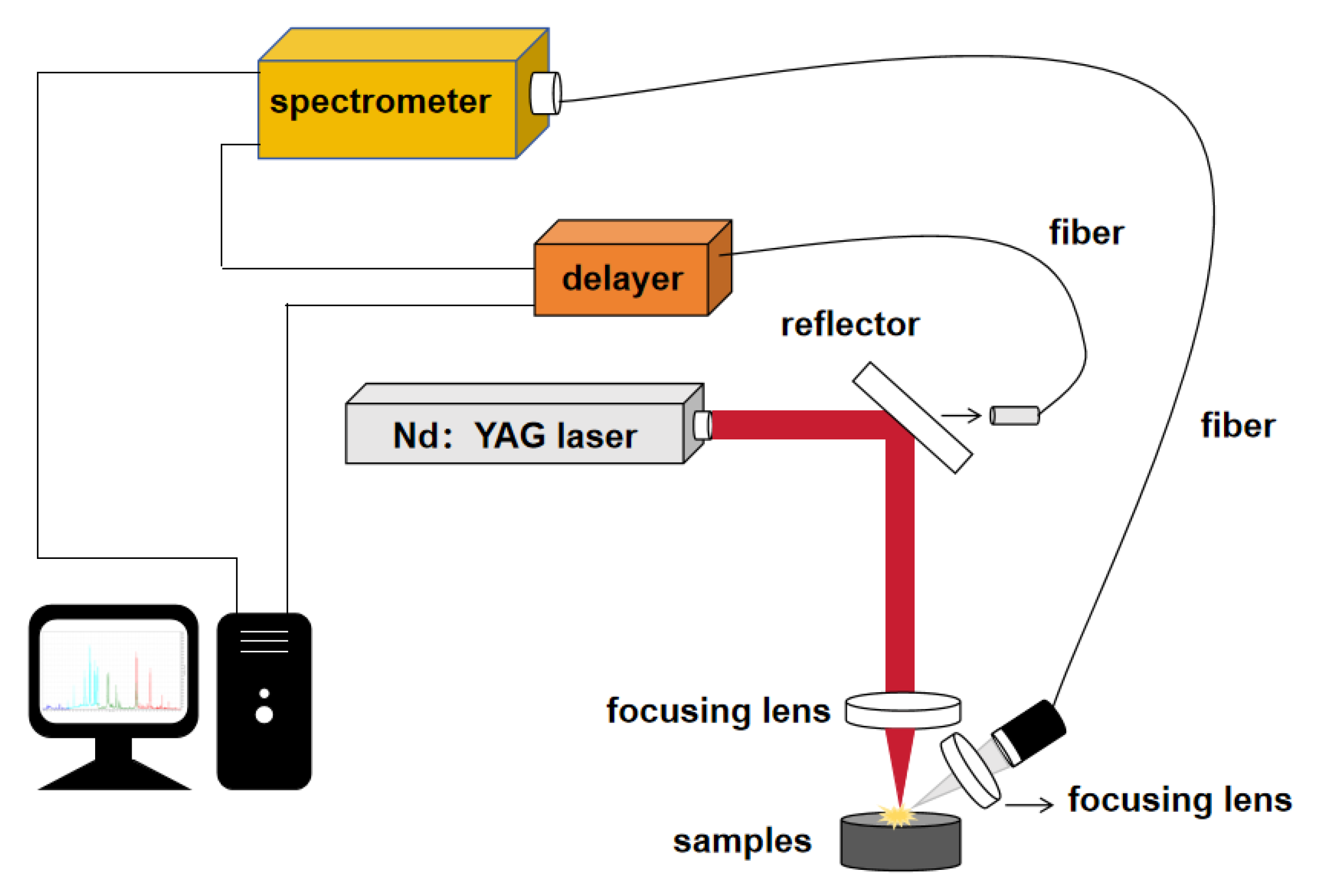
The laser-induced breakdown spectrum experimental system is shown in Figure 1, which includes the laser emission module, spectrum detection module, control module, and signal processing module. The passive Q-switched multi-pulse Nd:YAG laser produced by Ziyu Laser Technology Co., Ltd., of Anshan City, China, is used as the laser light source in the laser emission module. The working wavelength is 1064 nm, the repetition frequency is set to 1 Hz, and the pulse width is 20 ns. The spectral detection module comprises a spectrometer connected with a delay device, an optical fiber connected to the spectrometer, and an optical fiber probe connected to the end of the ray. The control module comprises a delay device and a receiving optical fiber. A small part of the output laser light passes through the reflector (the reflectivity is greater than 99%) as the source of the light trigger pulse of the delay device. Most of the energy is focused on the sample surface through the reflector and quartz lens (f = 25.4 mm). The plasma radiation generated by excitation is collected by the receiving lens, coupled into the fiber, and then collected into the spectrometer (AVS-DESKTOP-USB2) through the fiber. After receiving the light trigger pulse, the delay receiver controls the spectrometer in the external trigger mode to collect the spectrum and display the spectrum data on the computer through the data line.

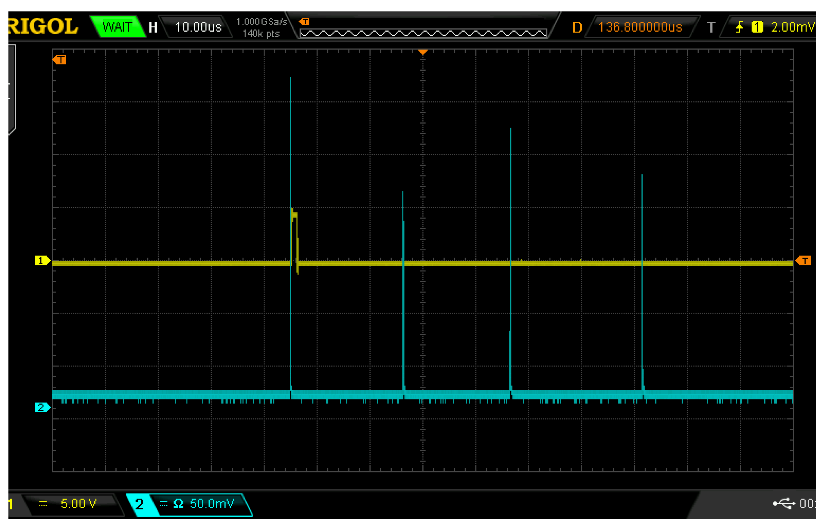
Inspired by two-pulse technology [22,23,24] and considering the cost of field detection equipment, we decided to use passive Q-switched lasers to construct a multi-pulse LIBS detection system. The calibrated pulse energy range of the Q-switched laser used in this system is 160–500 mJ. The passive Q multi-pulse Nd:YAG laser generates a pulse sequence composed of several independent high-energy short pulses, that is, each breakdown package contains several laser pulses, each pulse lasts for 20 ns, and the time interval between pulses is 15 to 30 μs. When the calibrated laser energy is 160 mJ, 4 laser pulses are issued. When the calibrated laser energy is increased, the number of pulses is also slowly increased. When the calibrated laser energy is its highest of 500 mJ, a maximum of 13 laser pulses are issued. The continuous background is subtracted using a baseline correction algorithm, and the spectrum is polynomially fitted to obtain the fitted spectrum. The fitting residuals are calculated, and peak removal is performed. If the actual value of the spectrum is greater than the fitted value, it is excluded; if the actual value is less than the fitted value, it is retained. After peak removal, the spectrum is again polynomially fitted, and the fitting residuals are calculated. If the conditions are met, the fitted spectrum, which serves as the baseline, is the output. If not, the spectrum reconstruction is repeated until the residuals meet the conditions, ultimately yielding the spectral baseline. Using polynomial fitting to obtain the baseline, the original spectrum is then subtracted from the baseline to produce the baseline-corrected spectrum. This process helps mitigate the impact of continuous background noise on experimental result analysis to some extent. In this experiment, the first pulse is selected as the trigger, with a delay time (relative to the first pulse) set to 1.5 μs, and the exposure time of the spectrometer set to 1.05 ms. When the laser emits light, the delay device delays the selected trigger pulse signal, using the delayed signal to drive the spectrometer to collect the plasma signal focused on the fiber optic by the receiving lens. The output pin of the delay device, which generates the delayed signal, is connected to an external trigger pin on the spectrometer, enabling precise control over the timing of different laser pulses and their corresponding delays in spectral acquisition. Although the output laser pulse energy of passive Q-switched laser is not as stable as that of active Q-switched laser, the operation of passive Q-switched laser is simple and the cost is low, which is more suitable for the integration of miniaturized equipment and suitable for field detection. The laser pulse width is 20 ns, and the time interval between different pulses is between 15 μs and 30 μs. The delay control module independently designed by the laboratory can realize the delay function and select multiple optical pulses, and then delay the selected pulses as trigger pulses. The delay unit converts the original optical pulse signals collected by photodiodes into electrical signals and then transforms them into corresponding TTL square wave signals through a gate driver. The photodiode used in the delay unit is an SFH209P-type photodiode with a working wavelength range of 400–1100 nm. The laser used in the experiment emits a wavelength of 1064 nm, which falls within its operating wavelength range. This photodiode has excellent time response performance, making it highly suitable for capturing optical signals. The voltage signal generated from the photodiode is an analog signal, which is further processed using a UCC27519 chip to convert the analog signal into a TTL signal. When the laser energy value is 160 mJ, the effect of using the delay device to select and delay the trigger pulse is shown in Figure 2, where the yellow waveform is the delay trigger signal and the blue waveform is the laser pulse signal. Each grid in the X-axis direction represents 10 μs, each grid in the Y-axis direction represents a voltage with an amplitude of 5 for the yellow waveform, and each grid in the Y-axis direction represents a voltage with an amplitude of 50 mV for the blue waveform.

In this experiment, the first pulse was selected as the trigger, the delay time (relative to the first pulse) was set to 1.5 μs, and the exposure time of the spectrometer was set to 1.05 ms. The delay device delays the selected trigger light pulse signal, and the delayed signal is used to drive the spectrometer to collect the plasma signal focused on the optical fiber by the receiving lens. The pin of the output delay signal of the delay device is connected with the external pin triggered by the external pin of the spectrometer, which can realize spectrum acquisition after different delays of different laser pulses.

In the LIBS experiment, a band of 196–220 nm was selected as the observation interval for background noise analysis. As shown in Figure 3, the LIBS spectral background of potassium dihydrogen phosphate aqueous solution in the range of 196–220 nm induced by one pulse is compared with the LIBS spectral background induced by 5 and 13 pulses using the liquid–solid conversion method of the graphite substrate.

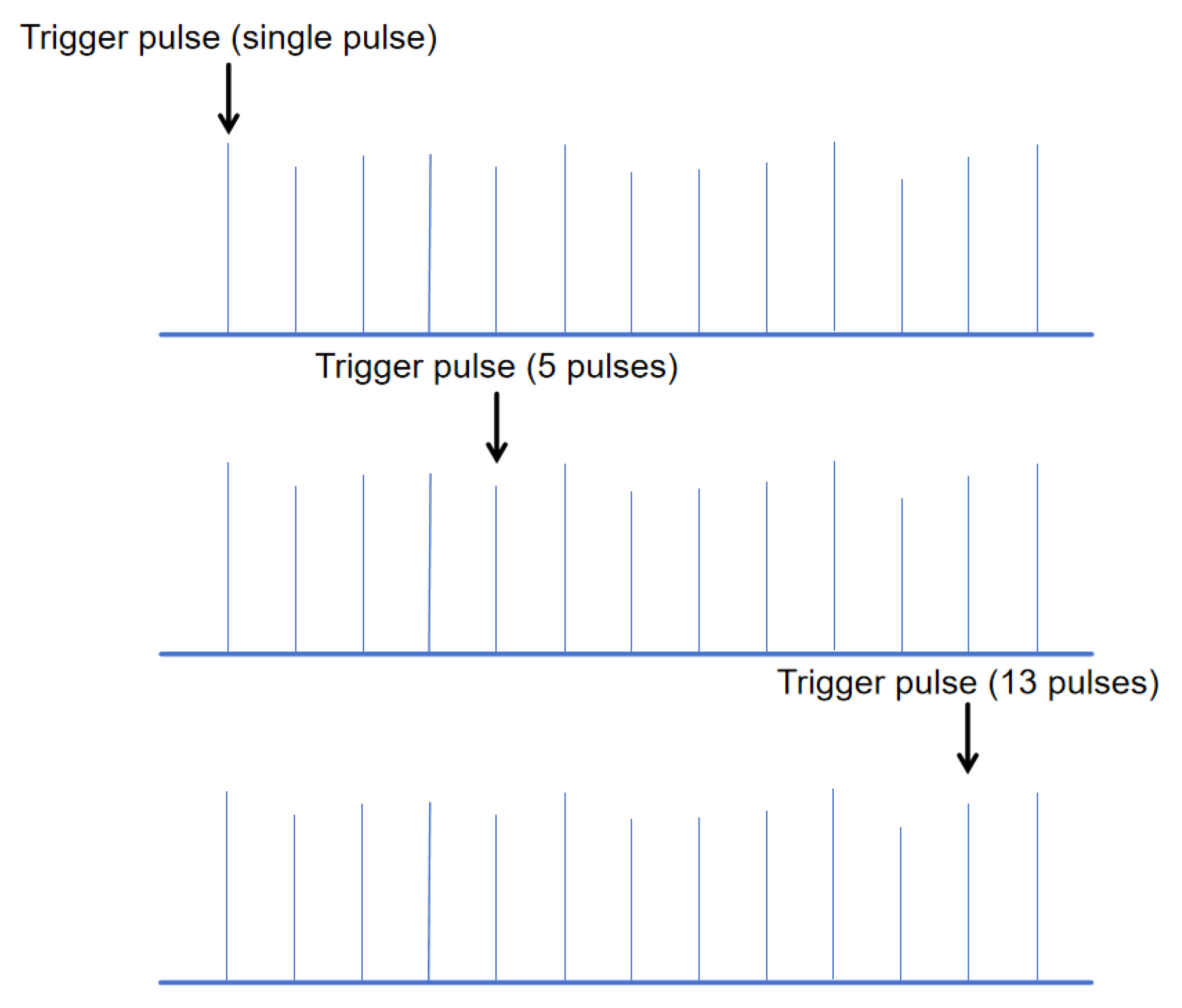
The schematic diagram of the trigger pulse position under different numbers of pulses is shown in Figure 4.

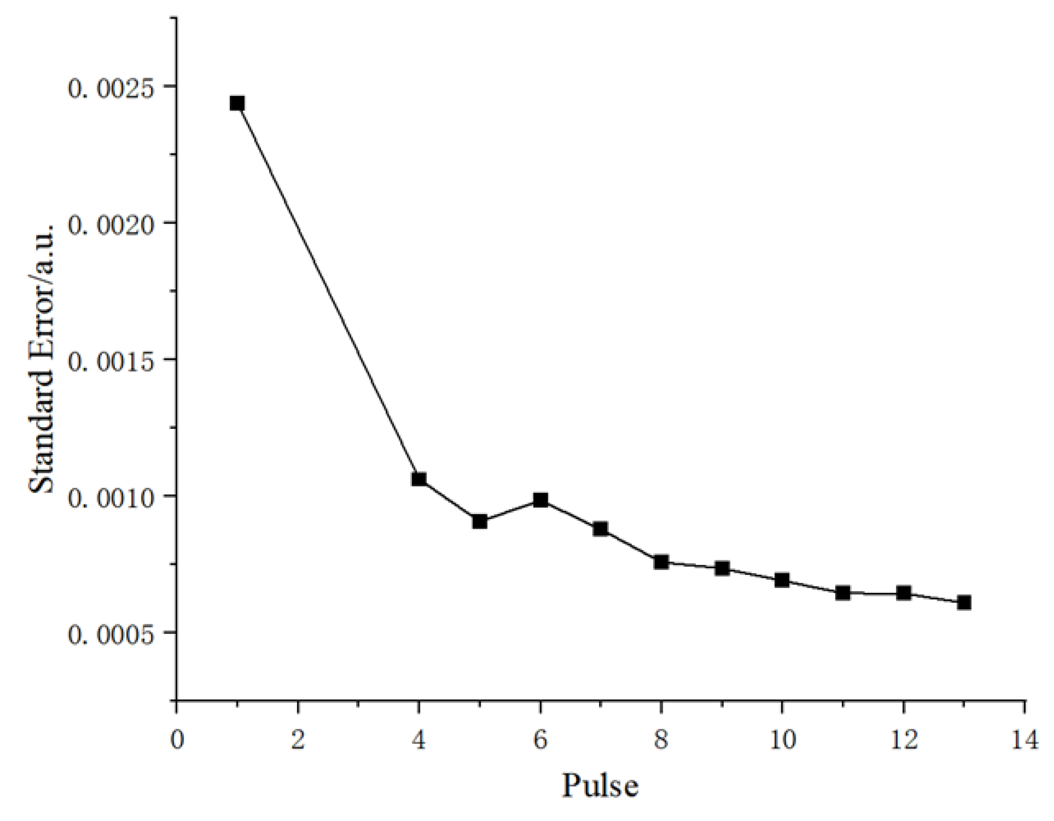
As can be seen from the figure, under the condition of a single pulse, the background noise of the obtained spectrum is strong, and the spectral background becomes smooth with an increase in the number of pulses. When the number of pulses is 13, the spectral background is the smoothest. When the number of induced pulses is 1, 4, 5, 6, 7, 8, 9, 11, 12, and 13, the changing trend of spectral background noise is shown in Figure 5.

According to the figure, the standard deviation of the spectral background noise decreases gradually with the number of induced pulses. This means that as the pulse increases, the dispersion of the background noise data gradually decreases and the data becomes more stable and concentrated. A comprehensive analysis of Figure 3 and Figure 5 shows that during a breakdown cycle, the increase in the number of pulses is accompanied by an increase in energy, leading to a decrease in the standard deviation of background noise and the continuous background baseline. Experimental verification confirms that an increase in the number of pulses (with higher laser energy) results in additional background noise, but the overall signal-to-noise ratio remains higher than when there are fewer pulses (lower laser energy). Considering the influence of the background noise of the LIBS line on the detection limit, this system selects 13 pulses, namely a laser with an energy of 500 mJ for the experiment.

This study proposes a PLS-SVR fusion quantitative analysis algorithm. First, random sampling and data augmentation are used to expand the small sample dataset, overcoming the limitations of limited experimental data in traditional LIBS. Then, Savitzky–Golay filtering and normalization preprocessing are introduced to eliminate plasma fluctuation noise. Next, PLS is employed to extract full-spectrum features and fuse the characteristic peak intensity values of nitrogen and phosphorus elements, balancing global features with key wavelength information. Finally, a Gaussian kernel SVR model is constructed, and hyperparameters are optimized through 5-fold cross-validation to achieve precise prediction of copper solution concentration. This approach fully leverages the advantages of SVR in small-sample nonlinear modeling, combined with the dimensionality reduction capability of PLS, enhancing adaptability to matrix effects while ensuring computational efficiency.

The core structure of the algorithm can be divided into three parts: multi-strategy data enhancement, feature space optimization, and nonlinear regression modeling.

Multi-strategy Data Enhancement: In response to the limited sample size of LIBS spectral data, an enhanced strategy based on random sampling integration (random sampling ensemble, RSE) is proposed. Random subspace sampling: for each concentration sample, 100 replications with replacement are performed on N spectra. Through 100 random samplings and noise addition, the original N spectra are expanded into 100 × N enhanced samples, increasing data diversity by combining differentiated spectral subsets. Noise injection enhancement: Gaussian white noise with a maximum intensity of 1% is added to the sampled spectra to simulate instrument noise fluctuations and environmental interference in actual measurements, enhancing robustness against minor variations. Spectral Morphology Optimization: The Savitzky–Golay filter (third-order polynomial, 7-point window) is used for spectral smoothing to suppress high-frequency noise while retaining peak position characteristics. This enhances the data and improves the signal-to-noise ratio. After area normalization, the impact of light source intensity fluctuations on absolute spectral intensity is eliminated, allowing the model to focus on relative intensity distribution rather than absolute intensity, thus enhancing adaptability to changes in equipment status.

Feature Space Optimization: For the high-dimensional characteristics of spectral data (8192 wavelength channels), PLS is used to reconstruct the feature space. Variable Projection: By maximizing the covariance between the spectral matrix X and the concentration vector Y, a latent variable space is constructed. The top 10 principal components (cumulative variance contribution > 95%) are selected to achieve feature compression from 8192 dimensions to 10 dimensions. Covariance Optimization: The objective function of PLS is shown in Equations (3)–(7), ensuring that the reduced features retain spectral variation information while being highly correlated with concentration variables.

$$\underset{w,c}{\max }\mathrm{cov}(X_w,Y_c)s.t.‖w‖=1,‖c‖=1$$

(1)

• $X\in {ℝ}^{n\times p}$: Spectral data matrix (n samples, p = 8192 wavelength points);
• $Y\in {ℝ}^{n\times 1}$: Concentration label vectors;
• $w\in {ℝ}^{p\times 1}$: Projection weight vectors for spectral variables;
• $c\in {ℝ}^{1\times 1}$: Projected weight scalar for concentration variables;
• $\mathrm{cov}(X_w,Y_c)$: Covariance of spectral score versus concentration score after projection.

Find the weight vector $w$ and $c$, such that the covariance between the projected spectrum and the concentration variable is maximized, while constraining the magnitude of the weight vector to 1 (to prevent the solution from becoming infinite). This process effectively eliminates spectral redundancy and reduces the risk of overfitting in the model. During feature space optimization, the spectral intensity data points of known nitrogen and phosphorus element characteristic lines are concatenated as additional features in the PLS-reduced feature space. This operation directly retains the original intensity information of key wavelength points, capturing local features that PLS might lose. On the basis of data-driven (PLS), this approach integrates prior knowledge, enhancing compatibility.

Nonlinear Regression Modeling: Based on the augmented feature space, construct a Gaussian Kernel SVR model. Kernel Function Mapping: Use the radial basis function (RBF) to map linearly inseparable features into high-dimensional space. Structural Risk Minimization: Balance empirical risk and model complexity by optimizing regularization parameters and kernel coefficients. Cross-Validation Tuning: Automatically optimize hyperparameters using 5-fold cross-validation to ensure the model’s generalization performance on unseen data. After training the model, preprocess and extract features from test samples (unknown concentration samples) and perform concentration prediction.

3. Experimental Detection

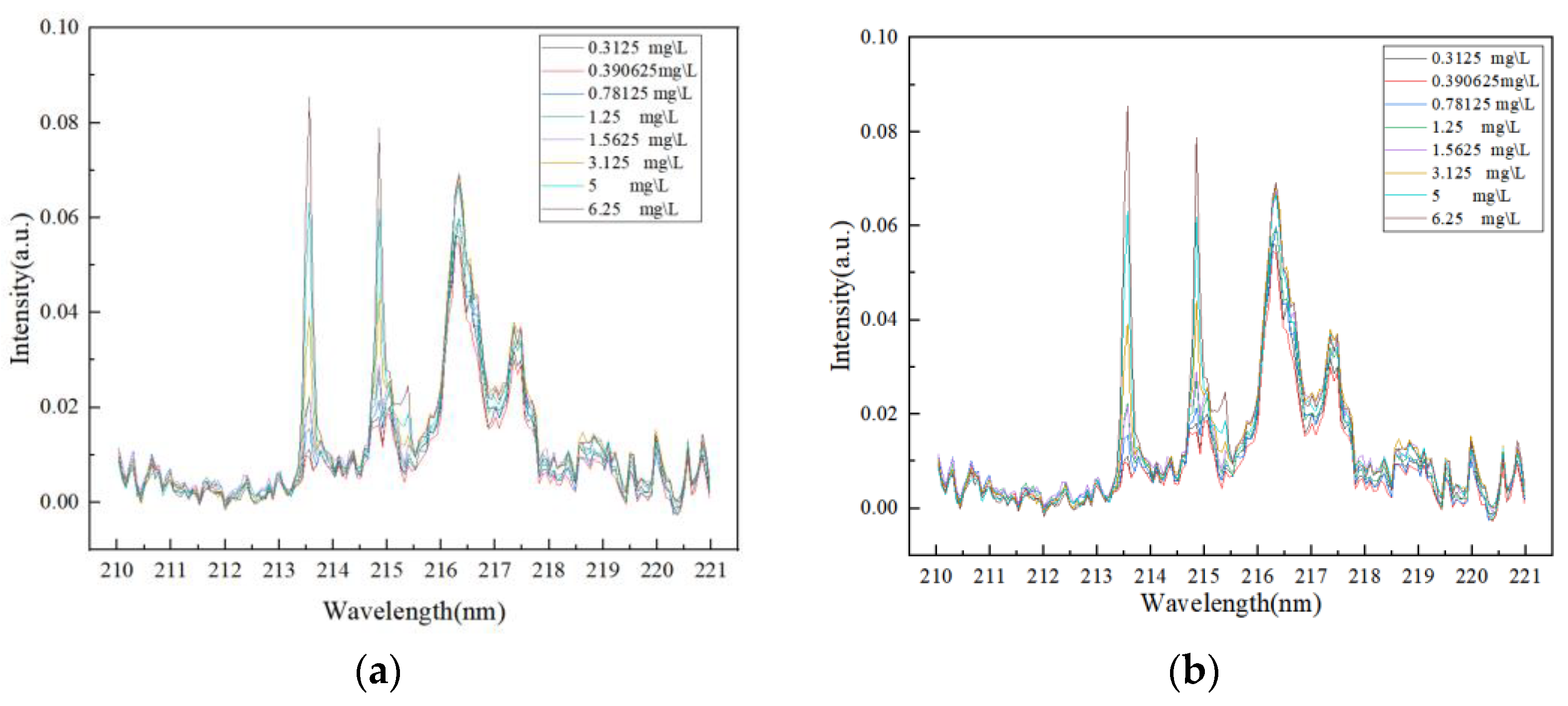
The sample solution containing P elements was tested using the LIBS experimental system shown in Figure 1, and P I 213.6182 nm and P I 214.9145 nm lines were selected as reference lines for the quantitative analysis of P elements. The laser experiment on graphite substrate was carried out with the LIBS instrument, and the spectral results obtained are shown in Figure 6.

In this spectral characteristic map, no significant peak signals were observed near the wavelength range of the P element characteristic line, mainly showing as noise disturbances. The intensity values of these noise signals are relatively stable and at a low level, causing no significant interference with the selected analytical peaks in this paper. Therefore, the spectral characteristics of this substrate meet the basic conditions for use as an enrichment substrate, meaning that the spectral background of the substrate itself will not significantly affect the detection of the target element. The P sample solution was evenly coated on the surface of the graphite substrate by the titration method and heated and dried. The laser dot operation was carried out on the treated graphite substrate by LIBS instrument, and the obtained spectral results are shown in Figure 7.

In this spectral feature map, obvious peaks appear near the wavelength range of the P element feature line. Comparing Figure 6, we can determine the peaks, namely the P I 213.6182 nm and P I 214.9145 nm spectral lines. According to Chinese national standards, the content limits of total phosphorus (TP) in water bodies are mainly based on the Surface Water Environmental Quality Standard (GB 3838-2002) [25] and the Comprehensive Sewage Discharge Standard (GB 8978-1996) [26]. The Surface Water Environmental Quality Standard (GB 3838-2002) divides surface water into five categories, as shown in

Table 1. Total phosphorus limit in the Surface Water Environmental Quality Standard (GB 3838-2002).

Water Quality Classification	$\mathbf{Class}\mathbf{I}$	$\mathbf{Class}\mathbf{II}$	$\mathbf{Class}\mathbf{I}\mathbf{I}\mathbf{I}$	$\mathbf{Class}\mathbf{IV}$	Class V
$\mathrm{Total}\mathrm{phosphorus}\mathrm{content}(\mathrm{m}\mathrm{g}·{\mathrm{L}}^{-1})$	≤0.02	≤0.1	≤0.2	≤0.3	≤0.4

, and different categories of water bodies have different restrictions on total phosphorus.

The Comprehensive Sewage Discharge Standard (GB 8978-1996) stipulates the discharge limits of total phosphorus in sewage as shown in

Table 2. The total phosphorus limit in the Comprehensive Sewage Discharge Standard (GB 8978-1996).

Pollutant	$\mathbf{P}\mathbf{r}\mathbf{i}\mathbf{m}\mathbf{a}\mathbf{r}\mathbf{y}\mathbf{S}\mathbf{t}\mathbf{a}\mathbf{n}\mathbf{d}\mathbf{a}\mathbf{r}\mathbf{d}$	Secondary Standard	Tertiary Standard
$\mathrm{Total}\mathrm{phosphorus}\mathrm{content}(\mathrm{m}\mathrm{g}·{\mathrm{L}}^{-1})$	≤0.5	≤1.0	≤2.0

, which is applicable to the discharge of industrial wastewater and urban sewage.

According to the above national standards and actual system detection capacity, the minimum concentration of phosphorus sample solution is set to 0.3125 $\mathrm{m}\mathrm{g}·{\mathrm{L}}^{-1}$ and the maximum concentration is set to 5 $\mathrm{m}\mathrm{g}·{\mathrm{L}}^{-1}$. The solute equipped with a phosphorus sample solution is potassium dihydrogen phosphate (analytical pure) produced by Tianjin Beichen Founder Reagent Factory, with a molecular weight of 136.09 and easily soluble in water. A total of 10 solution samples of different phosphorus contents were prepared, and the corresponding phosphorus contents of each group are shown in

Table 3. Phosphorus element content in the sample solution.

Sample Number	1	$2$	$3$	$4$	5
$$\begin{gathered} \mathrm{Phosphorus}\mathrm{content} \\ (\mathrm{m}\mathrm{g}·{\mathrm{L}}^{-1}) \end{gathered}$$	0.3125	0.390625	0.625	0.78125	1.25
Sample Number	6	7	8	9	10
$$\begin{gathered} \mathrm{Phosphorus}\mathrm{content} \\ (\mathrm{m}\mathrm{g}·{\mathrm{L}}^{-1}) \end{gathered}$$	1.5625	2.5	3.125	5	6.25

.

The detailed procedure is described as follows: (1) Stock Solution Preparation: A stock solution (100 mg/L P) was prepared by dissolving 0.4393 g of potassium dihydrogen phosphate (dried at 105 °C for 2 h) in ultrapure water. The solution was transferred to a 1 L volumetric flask and diluted to the mark. (2) Working Standard Solutions: Serial dilutions of the stock solution were performed to obtain 10 working standards (0.3125–6.25 mg/L P).

Titration and drying of the sample solution: The peristaltic pump is fixed at a height of 5.5 cm from the substrate surface, where droplets fall onto the substrate to form water stains with a diameter of approximately 0.7 cm, nearly circular in shape. A relay controls the peristaltic pump to drop the test solution onto the substrate surface. The flow rate of the peristaltic pump can be controlled by adjusting the DC power supply voltage; it is set to 0.2 mL every 60 s. Each sample group lasts for 60 s, or 5 drops. Place the substrate on a heating plate and set the temperature of the heating plate to 120 °C to heat the solution until it is completely dried (about 7 min). Through titration and drying treatment, elemental enrichment can be measured on the substrate surface. Use the system shown in Figure 1 for LIBS experiments, dotting the surface of the substrate to obtain multiple sets of spectral data.

In order to verify the practical application of the system, the LIBS system was applied to the actual water sample, and the results of other test means were analyzed. There were two actual water samples, numbers 1 and 2. The two groups of water samples were taken from the two artificial lakes in the south and north of the school. The sampling site is indicated by the red circle in Figure 8.

During the experiment, each water sample was added to the surface of the graphite substrate using the titration method. LIBS experiments were performed using the system shown in Figure 1 to dot the substrate surface of each actual water sample to obtain multiple sets of spectral data.

The experimental test results were verified using the 5B-6C multi-parameter water quality analyzer produced by Lianhua Technology. The detection standard for the total phosphorus of this instrument is the ammonium molybdate spectrophotometric method (GB 11893-89). The specific operation steps are as follows: (1) Take 8 mL of the water sample. (2) Add 1 mL of potassium persulfate, cover, tighten, and shake well. (3) Seal and digest at 120 °C for 30 min. (4) Cool in air for 2 min and then in water for 2 min. (5) Add 1 mL of LH-P1 reagent and shake well. (6) Add 1 mL of LH-P2 reagent, shake well, and let it stand for 10 min. (7) Perform the colorimetric reading.

The test results for phosphorus content in water samples No. 1 and No. 2 are shown in

Table 4. Test results of phosphorus content in water samples 1 and 2.

Number	$\mathbf{Phosphorus}\mathbf{Test}\mathbf{Results}(\mathbf{m}\mathbf{g}·{\mathbf{L}}^{-1})$
1	0.236
2	0.152

.

4. Results Analysis

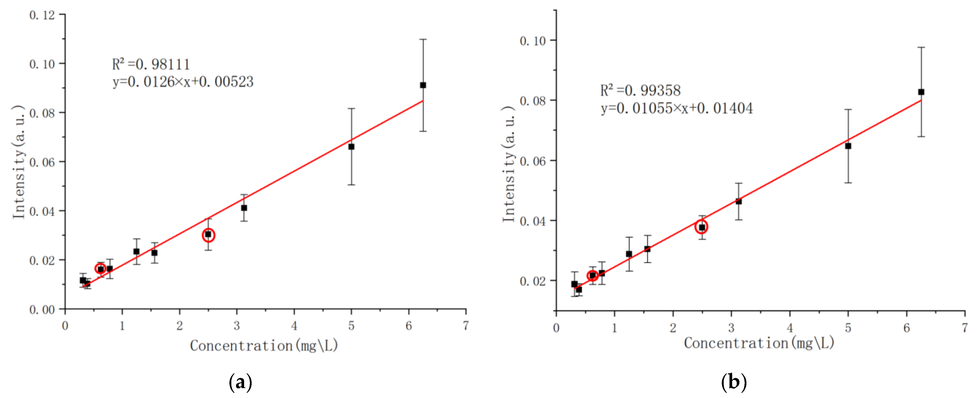
Sixteen laser experiments were conducted on each group of experimental samples. The obtained spectral data were preprocessed and averaged as the detection spectra of the samples in this group. After normalization and baseline correction, the ratio of the spectral intensity of phosphorus characteristic lines to that of carbon atomic lines at 247.856 nm in the spectra of each solution sample was extracted as the vertical axis, with the content of phosphorus to be measured in the solution sample as the horizontal axis. Linear fitting analysis was performed using Origin2022 software. The final calibration curve for phosphorus (P I 213.6182 nm and P I 214.9145 nm) is shown in Figure 9, where red circles mark the test samples and the other points represent the calibration samples.

The relative intensity of the characteristic spectral line of the above model has a good linear relationship with the content of the corresponding elements in the sample solution, and the effect is relatively ideal.

The detection limit ($LOD$) is an important index for evaluating the quantitative analysis of a single test [27]. Its value reflects the minimum detection value and ability of LIBS. The calculation formula is as follows:

$$LOD={\displaystyle \frac{3\sigma }{k}}$$

(2)

In the formula, σ is the standard deviation and k is the slope of the calibration curve. The $LOD$ value of the corresponding calibration curve was calculated based on the calibration curve shown in Figure 9.

The system uses the corrected root mean square error (${\mathrm{R}}_{\mathrm{M}\mathrm{S}\mathrm{E}}^{\mathrm{C}}$), predicted root mean square error (${\mathrm{R}}_{\mathrm{M}\mathrm{S}\mathrm{E}}^{\mathrm{P}}$), and average relative error ($\mathrm{M}\mathrm{R}\mathrm{E}$) as indicators. Combined with the element calibration fitting curve in Figure 9, the $\mathrm{M}\mathrm{R}\mathrm{E}$, ${\mathrm{R}}_{\mathrm{M}\mathrm{S}\mathrm{E}}^{\mathrm{C}}$, and ${\mathrm{R}}_{\mathrm{M}\mathrm{S}\mathrm{E}}^{\mathrm{P}}$ values of the corresponding calibration curve are calculated.The quantitative analysis parameters of the correction curve are shown in

Table 5. Calibration curve quantitative analysis parameters.

Spectral Lines to Be Analyzed/nm	${\mathbf{R}}^2$	$\mathbf{L}\mathbf{O}\mathbf{D}$$(\mathbf{m}\mathbf{g}·{\mathbf{L}}^{-1})$	$\mathbf{M}\mathbf{R}\mathbf{E}$ (%)	$$\begin{gathered} {\mathbf{R}}_{\mathbf{M}\mathbf{S}\mathbf{E}}^{\mathbf{C}} \\ (\mathbf{m}\mathbf{g}·{\mathbf{L}}^{-1}) \end{gathered}$$	$$\begin{gathered} {\mathbf{R}}_{\mathbf{M}\mathbf{S}\mathbf{E}}^{\mathbf{P}} \\ (\mathbf{m}\mathbf{g}·{\mathbf{L}}^{-1}) \end{gathered}$$
PⅠ213.6182 nm	0.98111	0.09	17.76	0.0546	0.1803
PI214.9145 nm	0.99358	0.23	12.31	0.0509	0.1406

.

To further improve the accuracy of phosphorus concentration prediction in unknown water samples, this paper employs a PLS-SVR fusion quantitative algorithm to conduct an in-depth analysis of experimental results. The cross-validation graph of the algorithm (true values and predicted values) is shown in Figure 10. The specific procedure is as follows: Using 10 sets of spectral data with different phosphorus concentrations obtained from experiments as samples, each set contains 16 test data points. The two sample sets with concentrations of 0.625 mg/L and 2.5 mg/L are designated as the prediction sets, while the remaining eight sets serve as the training sets for experimentation. All sample data undergo preprocessing steps such as normalization and baseline correction. The training set is used for model building and training, while the average of the two prediction sets serves as the true spectrum for the 0.625 mg/L and 2.5 mg/L concentrations, which are used for concentration prediction after model training. The average spectra of the training set before and after sample expansion are shown in Figure 11.

The average spectrum of the forecast set is shown in Figure 12.

The prediction results of this system are shown in

Table 6. The prediction results of the PLS-SVR fusion quantitative algorithm model.

Predict the True Concentration of Samples	$\mathbf{Predicted}\mathbf{Concentration}(\mathbf{m}\mathbf{g}·{\mathbf{L}}^{-1})$	$\mathbf{Relative}\mathbf{Error}\left(\mathbf{\%}\right)$
0.625	0.6119	2.1
2.5	2.3608	5.6

.

The prediction results of the traditional linear regression method are shown in

Table 7. The relative error of two calibration curves for the traditional linear regression method was predicted.

Predict the True Concentration of Samples	PⅠ213.6182 nm	PⅠ214.9145 nm
0.625	35.6%	15.1%
2.5	20.4%	10.6%

. It can be seen that compared with traditional linear regression, SVR reduces the prediction error by handling the complex nonlinear relationship between concentration and spectrum through kernel techniques. The cross-validation results (MSE = 0.0233 ± 0.0144) confirm the stability of the model.

The prediction results of 0.625 mg/L and 2.5 mg/L phosphorus solutions showed that the relative errors were 2.1% and 5.6%, respectively, which reduced the errors by at least 86% and 47% compared with the traditional linear regression method. Combined with the concentration prediction model generated by the above training, the actual water samples were tested using the PLS-SVR fusion quantitative algorithm, and the predicted concentration of the phosphorus element and its detection error compared with the chemical method (spectrophotometry) detection instrument was obtained, as shown in

Table 8. The PLS-SVR fusion quantitative algorithm was used to detect the actual water samples to obtain the predicted phosphorus concentration and its detection error.

Water Sample Number	$$\begin{gathered} \mathbf{Phosphorus}\mathbf{Content} \\ (\mathbf{m}\mathbf{g}·{\mathbf{L}}^{-1}) \end{gathered}$$	$$\begin{gathered} \mathbf{Absolute}\mathbf{Error} \\ (\mathbf{m}\mathbf{g}·{\mathbf{L}}^{-1}) \end{gathered}$$	$\mathbf{Relative}\mathbf{Error}\left(\mathbf{\%}\right)$
1	0.2321	0.0039	1.6
2	0.1351	0.0169	11.1

.

It can be seen that the absolute error of phosphorus detection results in this system can be controlled within 0.017 mg/L, and the relative error can be controlled within 12%, which has a high detection accuracy.

At the same time, the experimental results above validate the following advantages of the PLS-SVR fusion quantification algorithm: (1) Small sample adaptability. Expanding the training set through data augmentation alleviates the bottleneck of limited sample sizes in LIBS experiments. The original training set contained only 16 samples per concentration, but after enhancement, 1600 data sets were generated, significantly improving the model’s generalization ability. (2) Noise suppression capability. The combined application of Gaussian noise injection and Savitzky–Golay filtering effectively suppresses the impact of plasma fluctuations and instrument noise on spectral signals, making the stability of prediction results significantly better than traditional methods. (3) Enhanced interference resistance. Traditional methods rely on a single spectral line intensity ratio (such as the C I 247.856 nm internal standard method), which is susceptible to matrix interference, whereas PLS-SVR utilizes full spectral information, automatically selecting key wavelengths through feature selection, reducing the influence of matrix differences on predictions. Moreover, PLS dimensionality reduction reduces the data dimensions from 8192 to 10, greatly decreasing the computational complexity of SVR while retaining over 95% of the spectral variation information and balancing accuracy and efficiency.

5. Conclusions

This study addresses the issue of insufficient sensitivity in liquid sample laser-induced breakdown spectroscopy (LIBS) for detecting phosphorus in water by proposing an enhanced strategy based on liquid–solid conversion using a graphite substrate, combined with the PLS-SVR fusion quantitative analysis algorithm, significantly improving detection performance. By optimizing the parameters of a passive Q-switched multi-pulse Nd:YAG laser system (pulse energy 500 mJ, 13 pulses), the plasma excitation efficiency and spectral signal-to-noise ratio were effectively improved. The application of the graphite substrate, through adsorption enrichment and interference suppression characteristics, reduced the detection limits of phosphorus characteristic lines (PI213.6182 nm and PI214.9145 nm) to 0.09 mg/L and 0.23 mg/L, respectively, with the highest coefficient of determination (R²) for calibration curve fitting reaching 0.99358, verifying the stability and reliability of the method. In actual water sample testing, the absolute error of this method was controlled within 0.017 mg/L, with a relative error below 12%, showing high consistency with traditional total phosphorus detection results. Further research indicates that the PLS-SVR fusion algorithm significantly reduces prediction errors in small-sample nonlinear modeling through data enhancement, noise suppression, and full-spectrum feature extraction (for example, the relative errors for 0.625 mg/L and 2.5 mg/L samples are reduced to 2.1% and 5.6%, respectively), demonstrating a significant improvement over traditional linear regression methods. The breakthrough of this technology lies in simplifying the pretreatment process (single sample preparation time <10 min), enabling rapid in situ monitoring of phosphorus pollution in water bodies. This provides an efficient and low-cost technical means for the precise management of eutrophic water bodies. Future research can focus on surface modification of graphite substrates, optimization of multi-element simultaneous detection, and enhancement of machine learning model generalization capabilities, further expanding their applicability in complex environmental matrices and promoting the large-scale application of LIBS technology from laboratory settings to environmental monitoring sites.