Structural Health Monitoring by Fiber Optic Sensors

Abstract

Although a crack creates a significant strain field at its tip, its effect on the strain field becomes nearly negligible only a few centimeters away from the crack, which complicates the task of damage detection. Two approaches are currently in use. The first one is a local approach that can detect damage if it intersects the optical fiber path; it is straightforward to implement but is limited to cases where the potential damage location can be anticipated (for example, in a concrete beam under flexural loads or around aircraft cargo doors). The second one, a global approach, seeks to identify damage anywhere in the structure by detecting subtle changes in the field of global strain. There is a need for algorithms to compare the strain dataset before and after damage. Machine learning offers tools to achieve this, but these tools have to be carefully selected to achieve good damage detectability. In this paper, we compare algorithms based on multivariate data analysis as well as data processing using neural networks, comparing their performance on a real structure.

1. Introduction

Fiber Bragg Gratings (FBGs) began to be used as strain sensors in the early 1990s, and approximately a decade later, fiber distributed sensing techniques based on Rayleigh or Brillouin backscattering became available. Since then, many large-scale structural tests and in-service strain and load measurements have been performed using fiber optic sensors, which exploit advantages over conventional sensors. This technology is now considered mature. To illustrate this point, several examples are included in this paper. For a system to function as a Structural Health Monitoring (SHM) system, it must incorporate some damage detection capability. Damage is defined as a localized change in a structure that reduces its strength and must be identified by comparing physical measurements taken before and after the damage occurs. In addition to strain measurements, data processing algorithms are needed to detect the onset of damage.

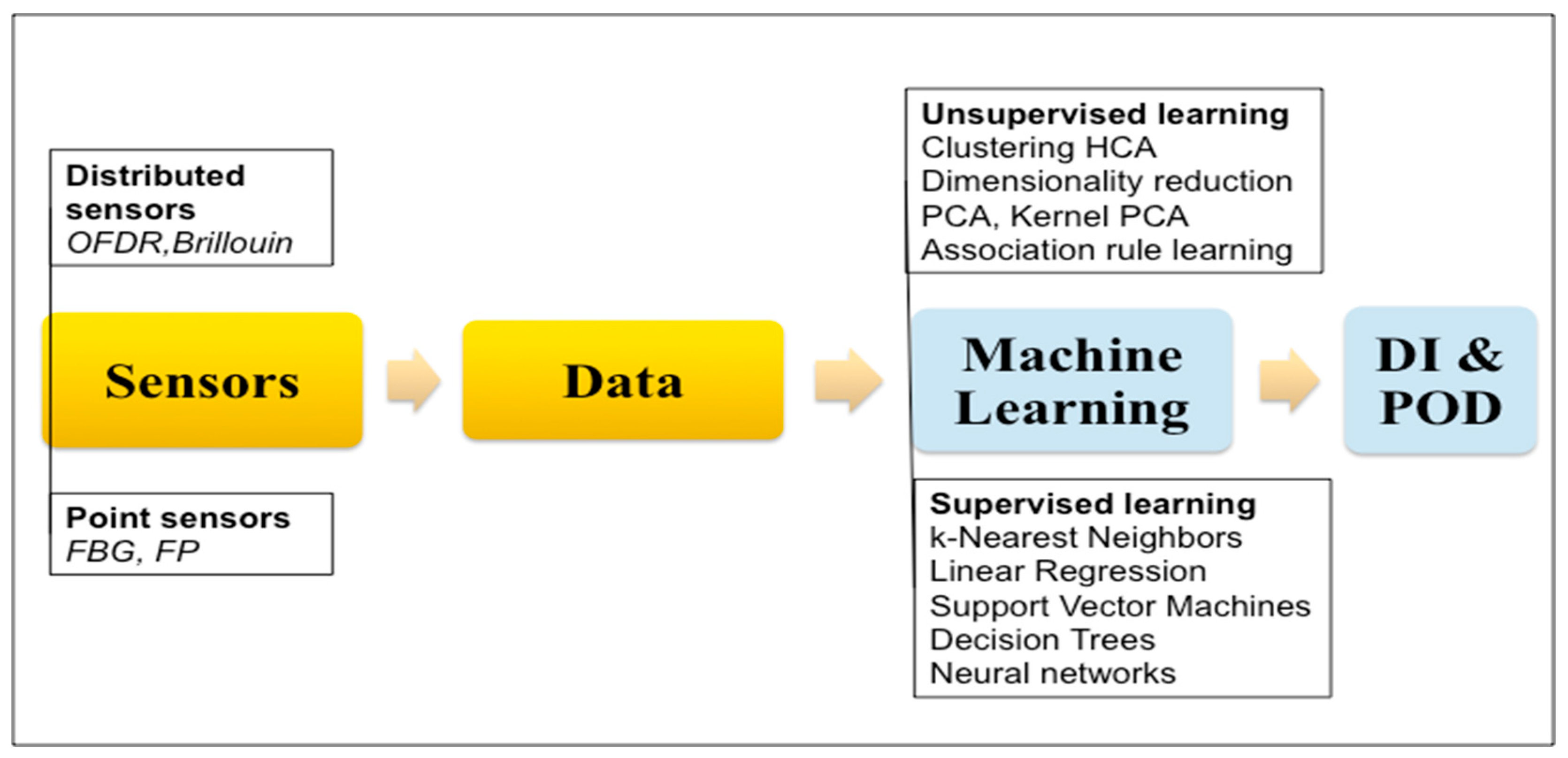
A search in the Scopus database yields more than 3000 documents under the keywords “Structural Health Monitoring Fiber Optic Sensors,” yet a significant percentage of these focus solely on fiber optic sensors, neglecting the broader concept of SHM—namely, automatic sensing with a large number of sensors followed by a diagnosis of the structure’s health based on the collected data, as outlined in Figure 1. Although the sensors and data acquisition define the SHM system, the critical aspect lies in the signal processing and information management. SHM is inherently multidisciplinary; an excellent overview of different techniques applied to aircraft structures is provided in [1]. For civil engineering structures, [2] compiles recent cases and outlines current challenges, although most examples focus on instances where cracks intersect the optical fiber path. For a more general approach, the integration of Artificial Intelligence (AI) into SHM is still in its early stages. This integration offers the prospect of self-improving systems capable of handling large datasets and detecting anomalies. This article presents a practical example of such integration. A global overview of the necessary tasks is shown in Figure 1.

When discussing fiber optic sensors, it is essential to acknowledge the three groundbreaking innovations that paved the way for this technology. The first was the invention of the optical fiber in 1965 by Chinese scientist Dr. Charles Kao, who was awarded the Nobel Prize in 2009 in recognition of this invention. The second major advancement was made by Dr. Hill from Canada, who discovered the photosensitivity of optical fibers, thereby enabling the production of fiber Bragg gratings—the most widely used fiber optic sensor. The third significant breakthrough occurred 20 years later in 1998, when Dr. Froggatt, working for NASA Langley in the United States, pioneered the field of distributed sensing, which offers significant advantages over point sensing.

A good review on the conceptual aspects of machine learning for fiber optic sensor applications is available in [3].

This paper is organized as follows: Section 2 is a short discussion on fiber optic sensors and their applications for strain measurements. Section 3 deals with local damage detection by DFOSs, while Section 4 illustrates global damage detection procedures, using both supervised and unsupervised learning on data obtained from experiments performed on a real structure instrumented with fiber optic strain sensors, tested before and after increasing levels of damage. Details to build a digital twin of the real structure are given, and conclusions drawn from this analysis are summarized in Section 5.

2. Fiber Optic Strain Sensors

The primary objective of any structural analysis is to determine the strains and stresses at every point in the structure. Although strains can be measured experimentally using point sensors, one-dimensional line sensors, or two-dimensional surface measurements, stresses cannot be directly measured and must be inferred from strain measurements via Hooke’s law. It is important to remember the tensorial nature of strain; in principle, six independent terms are required at every point in the structure. In practice, however, these are reduced to three components (namely, in-plane longitudinal, transverse, and shear strains) when measuring on the surface of a structure.

In the field of aeronautics, strain measurements serve three main purposes. The first one is to verify and validate new designs. Each new aircraft must undergo hundreds of tests on structural details to confirm theoretical calculations; these tests are instrumented with strain sensors, ranging from small-scale components to full-scale aircraft structural tests under static and dynamic loads. The second application is fatigue management, which is critical for aircraft safety. Modern aircraft are equipped with Lifetime Monitoring Systems that sometimes use strain gauges to record structural loads—including overloads, hard landings, and cycle accumulations. These data enable operators to better track usage and associated fatigue, thereby facilitating a more efficient maintenance schedule. The third application throughout the aircraft’s life is damage assessment for incipient cracks, a process known as SHM, which is still under development.

A similar approach is being adopted for civil infrastructures. Both new and existing large structures are now being instrumented with a wide variety of sensors due to reduced sensor costs and advances in wireless technology. Modern bridges, for example, commonly incorporate over 1000 sensors of various types—including accelerometers, strain gauges, GPS devices, image analysis systems, and many others. Recent advances in Big Data and AI allow for better exploitation of the continuous flow of raw data. Tools developed for Big Data analytics are well suited to handling such vast and high-dimensional datasets. The term “Big Data” is used to describe large volumes of complex data that must be analyzed within a short period.

2.1. Optical Fiber Bragg Gratings (FBGs)

Optical fiber Bragg gratings function as point sensors that are typically 1–10 mm in length, measuring strain along the fiber’s longitudinal direction, and can be easily multiplexed. Their performance is similar to that of conventional electrical strain gauges (ESGs). However, strain gradients along the grating and transverse stresses can distort the reflected optical peak [4]. This phenomenon must be carefully understood, particularly when FBGs are embedded in composite laminates. Although FBG technology has been available since the early 1990s, it is now regarded as mature (TRL 8), with the remaining challenges being certification and regulatory acceptance. Additionally, compact and rugged interrogation systems are currently available for in-flight measurements.

2.2. Distributed Fiber Optic Sensors (DFOSs)

Distributed fiber optic sensors provide strain measurements continuously along the entire length of the optical fiber, with a microstrain resolution comparable to that of FBGs or ESGs. Equipment based on Rayleigh scattering—commonly referred to as Optical Frequency Domain Reflectometry (OFDR)—offers spatial resolution in the order of millimeters, which is considerably better than that obtainable with Brillouin systems. However, OFDR’s drawbacks include a shorter measurement range (approximately 100 m as opposed to several kilometers for Brillouin systems) and relatively long acquisition times, thereby limiting its use to static and low-frequency measurements.

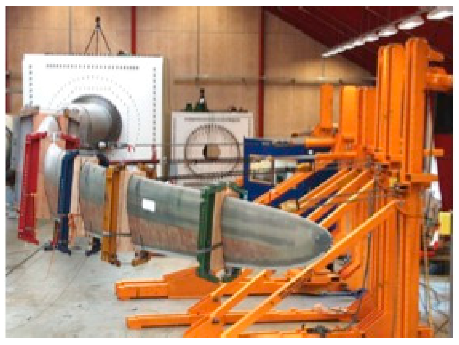
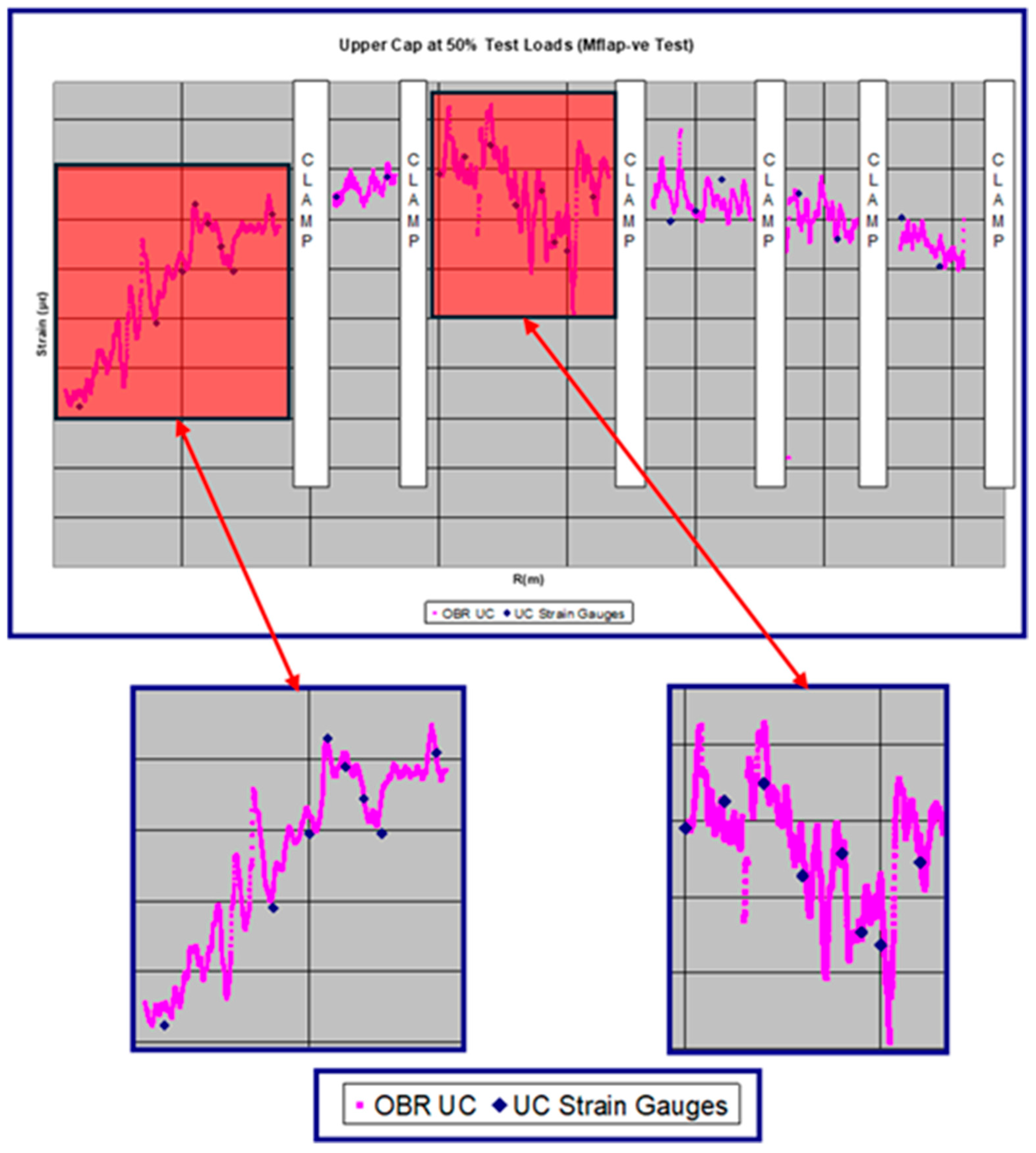
To illustrate the capabilities of DFOSs, Figure 2 shows a structural test conducted on a 45 m wind turbine blade equipped with five optical fibers bonded to its surface, along with conventional strain gauges. Not only was there excellent agreement between the two types of measurements (see Figure 3), but the test setup was also considerably simplified (bonding five straight optical fibers versus managing 160 ESGs and their cabling).

Moreover, DFOSs provided information that could not have been otherwise obtained. The continuous strain readings along the fiber (with a spacing of 1 mm) allowed for the early detection of local buckling when loads reached 65% of the maximum test load, ultimately enabling the test to be halted and averting structural collapse. Full details are provided in [5]. Numerous additional examples are available in the literature. The website of a commercial equipment supplier [6] contains information on real-life applications in aerospace, civil, and geotechnical engineering, as well as in the energy sector (including offshore platforms) and the railway and automotive industries.

3. Damage Detection

The established levels for an SHM system include the following:

Level 1.

Damage detection.

Level 2.

Damage location.

Level 3.

Damage classification and quantification.

Level 4.

Prognosis of residual strength.

3.1. Local Damage Detection

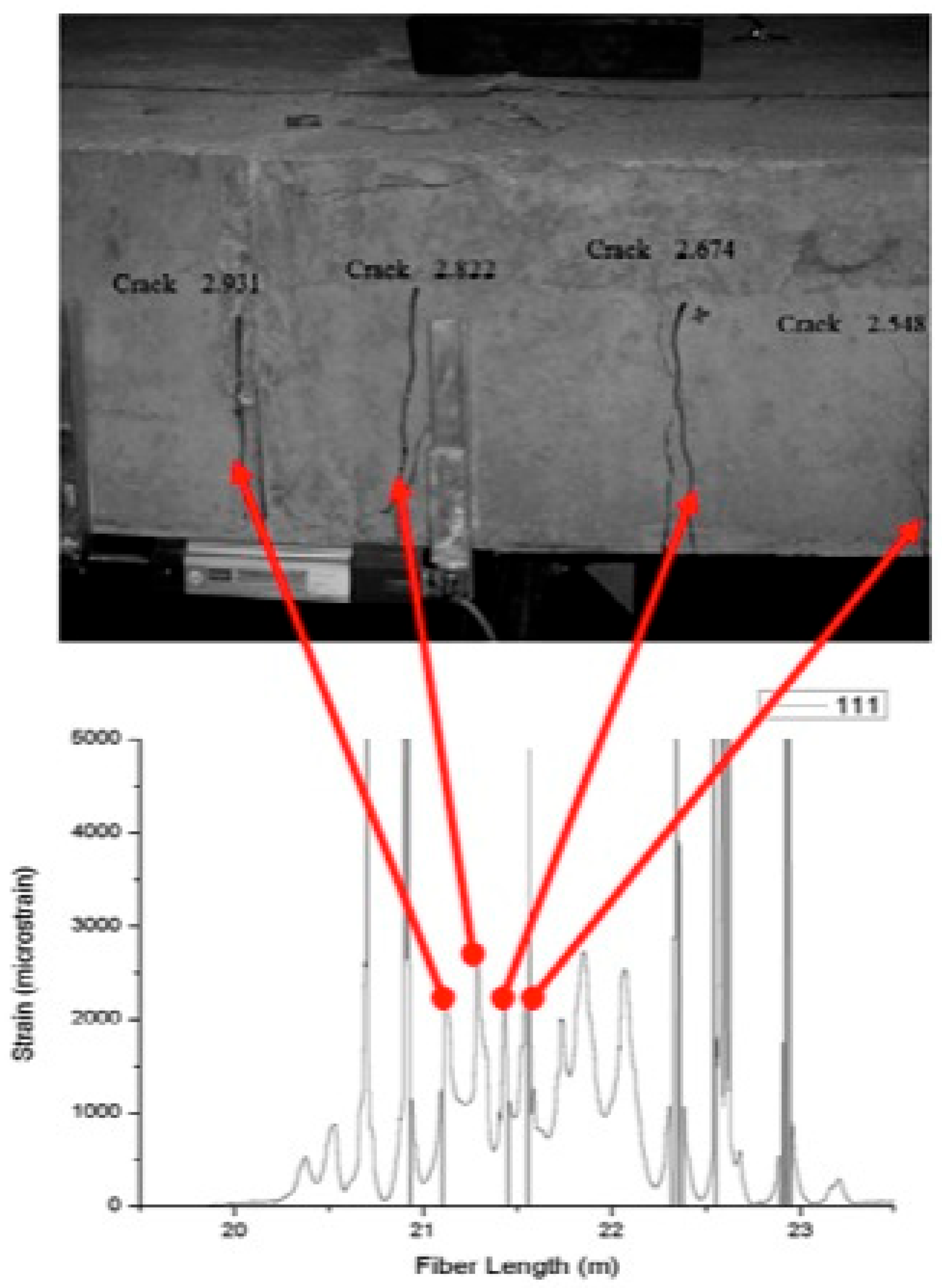
One of the earliest experiments utilizing DFOSs for damage detection was presented at ref [5]. In that study, a 7 × 2 m concrete slab under flexural loads was instrumented with optical fibers bonded to both the upper and lower surfaces. Due to the brittle nature of concrete, cracks appeared on the tensile side under relatively low loads. Concurrently, peaks in the strain distribution—recorded by the optical fiber on that surface—were observed. Although the average strain was rather low (approximately 50 microstrains), the segment of the optical fiber bridging a crack experienced significantly higher local strain due to the crack opening. As the load increased, both the number of cracks and corresponding strain peaks increased; the strain data were then used to accurately identify the number and positions of these cracks (Figure 4). Since then, this approach has been applied to many other civil structures, as reported in [2].

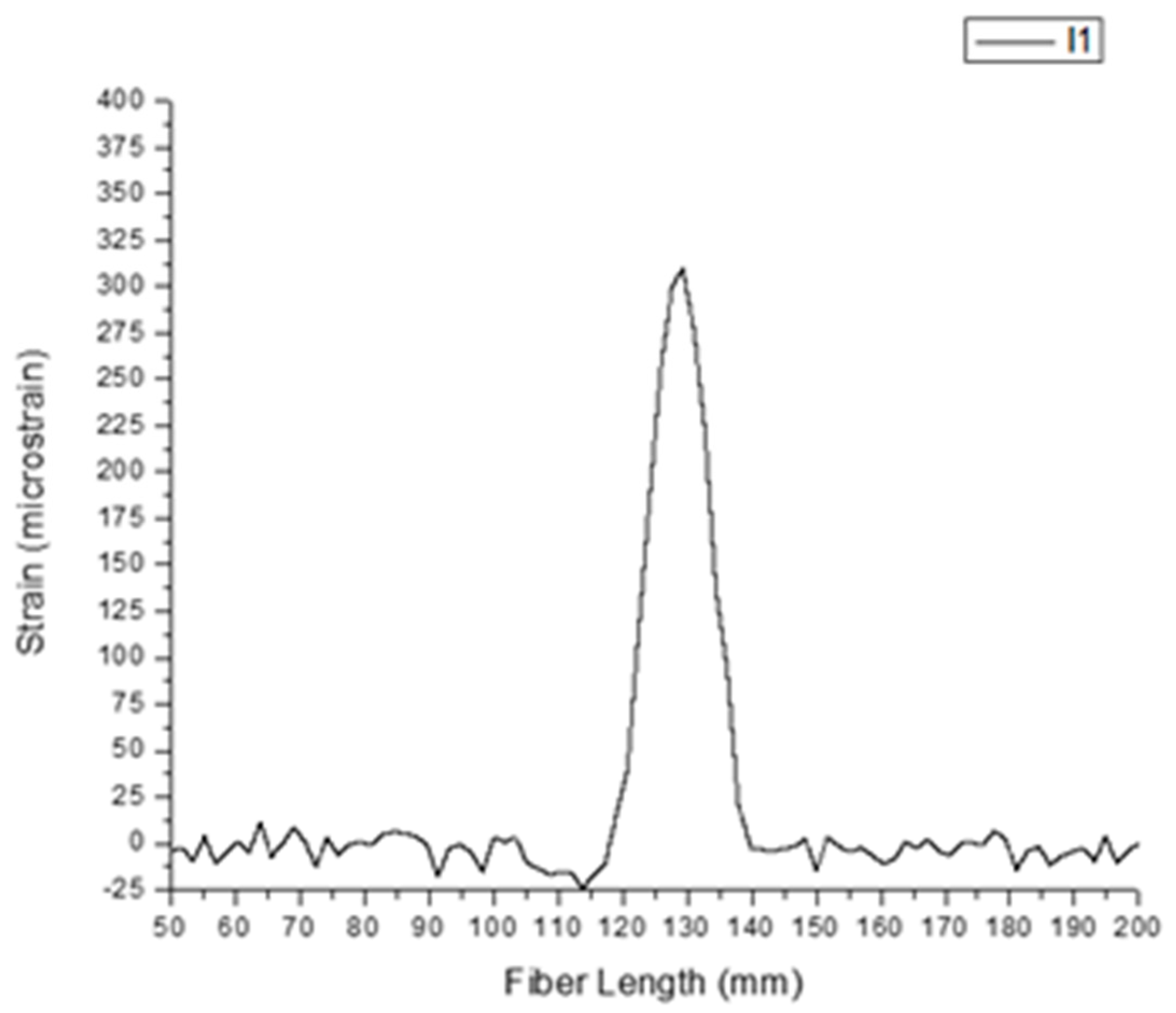
Although composite structures are not as brittle as concrete, a similar concept can be applied to damage detection following an impact—the most common threat to composites. Impact-induced delamination produces a permanent change in the strain field in the damaged area. This is demonstrated in Figure 5, which shows the strain distribution measured by an optical fiber bonded to a laminate following an impact, and is documented in [7]. The observed strain changes are attributed to internal residual strains released by the delaminations caused by the impact; the delaminated area, as confirmed by ultrasonic inspection (Figure 6a), corresponds closely with the region where the altered strains are measured. When the optical fiber is bonded to the backside of the laminate along a winding path—with optical lines spaced 5 mm apart—a strain map can be produced (Figure 6b) that almost precisely matches the ultrasonic image.

This approach may prove useful for SHM in areas known to be susceptible to damage—such as near manholes or around cargo doors—or for concealed areas that require disassembly for inspection, such as internal ribs with stiffeners. This procedure is the first reported usage of SHM by DFOSs in serial production, as applied by the Israeli Air Force to verify wing integrity on High-Altitude Long Endurance (HALE) Unmanned Aerial Vehicles (UAVs) [8].

3.2. Global Detection of Damage by Strain Measurements

The local approach described earlier detects only the damage that produces a significant strain change on the sensor, and there is no need for further processing to identify and locate the damage. In these cases, the sensor must be positioned coincidentally with the damage. For a more general scenario in which damage may occur anywhere in the structure, a different approach is required. A network of strain sensors distributed throughout the structure and subjected to an external load will provide strain data with high accuracy. Localized damage, such as delamination, may alter the strain field only at the impact point, with little to no measurable effect a few millimeters away. Consequently, the sensor network might not detect such damage unless it is large enough to alter the load path of the structure. The detection threshold depends on the severity of the damage, the applied loads, the number and proximity of sensors to the damage location, and, importantly, the sensitivity of the algorithm used to compare the current strain data with a baseline dataset collected from the undamaged structure under identical loading conditions.

4. Machine Learning for Damage Detection

Machine learning is a subset of AI that focuses on algorithms to “learn” information directly from data without relying on equations obtained from a physical model.

Different algorithms have been proposed, which can be broadly categorized into two groups, as sketched in Figure 1. The first group is based on unsupervised learning techniques to identify differences between two datasets. Because the number of sensors must be large and tests must be repeated to achieve statistical significance, multivariate data analysis methods are used; the most commonly employed is Principal Component Analysis (PCA). PCA is a robust algorithm that does not require any prior assumptions about the type of damage and produces, for each new dataset, a single scalar known as the “Damage Index” (DI), which quantifies the deviation of the new data from the baseline measurements.

The second group is supervised learning techniques, which include algorithms such as those based on Artificial Neural Networks (ANNs), among others. The performance of an ANN is strongly dependent on the quality and volume of data available from both the pristine and damaged structures. When a sufficiently large number of simulated cases are available for training, the ANN can accurately predict and classify damage. These algorithms become more accurate as more training data are provided to them.

It is important to clarify that both algorithms are considered data-driven; they do not require prior knowledge of the underlying physics governing the structural behavior.

4.1. Principal Component Analysis (PCA)

The following outlines the process for detecting damage from experimental strain measurements by using PCA when the physical structure is available:

• Sensor Network Deployment:

A sufficient number of sensors must be distributed throughout the structure to ensure complete coverage. When the structure is loaded, each sensor records a single strain measurement. The sensor closest to the damage location will record a higher strain change due to the localized influence of the crack, although these changes are often subtle and diminish rapidly with distance.

• Baseline Data Acquisition:

For the undamaged structure, the desired loads are applied, and the sensor responses are recorded. This process is repeated multiple times to ensure statistical significance and store the data in a matrix of dimensions (m × n), where m is the number of sensors and n is the number of experiments. The original data are re-expressed on a new orthogonal basis where they are arranged along directions of maximal variance and minimal redundancy, known as principal components.

• Post-Damage Data Collection:

After the occurrence of damage, the same loads are applied, and new strain measurements are acquired. Minor differences compared to the baseline data may occur but are typically not discernible by visual inspection due to small changes and measurement noise.

• Algorithm Application:

Apply an algorithm to compare the datasets obtained before and after damage. The algorithm will reduce the extensive data to a few numerical values or even a single scalar, known as the “Damage Index” (DI), the value of which increases when the new strain data deviates from the original undamaged data.

• Statistical Analysis:

Due to measurement noise, even repeated tests on the undamaged structure yield a nonzero DI; however, these values follow a standard distribution with low mean values. For cases involving damage, the DI correlates with both the size and location of the damage, provided the damage is sufficiently large to be distinguished with a high probability of detection.

It is worthwhile mentioning that PCA is also used for other purposes, such as the compression of data without the loss of significant information. It is available as a MATLAB 2023b tool, so there is no need for programming. It is only necessary to prepare the data columns, and the only output needed for SHM is a Damage Index, known as the Q-Index in PCA terminology, which measures whether the new dataset fits with the original data. Due to its easy implementation and fast processing, it is a very widespread SHM analysis method. The Doctoral Thesis of Julian Sierra [9] was one of the first works completed on the application of PCA to fiber optic sensor data. Since then, the algorithm has been applied by several authors to different kinds of structures [10,11,12,13,14,15,16,17,18], with a high degree of success.

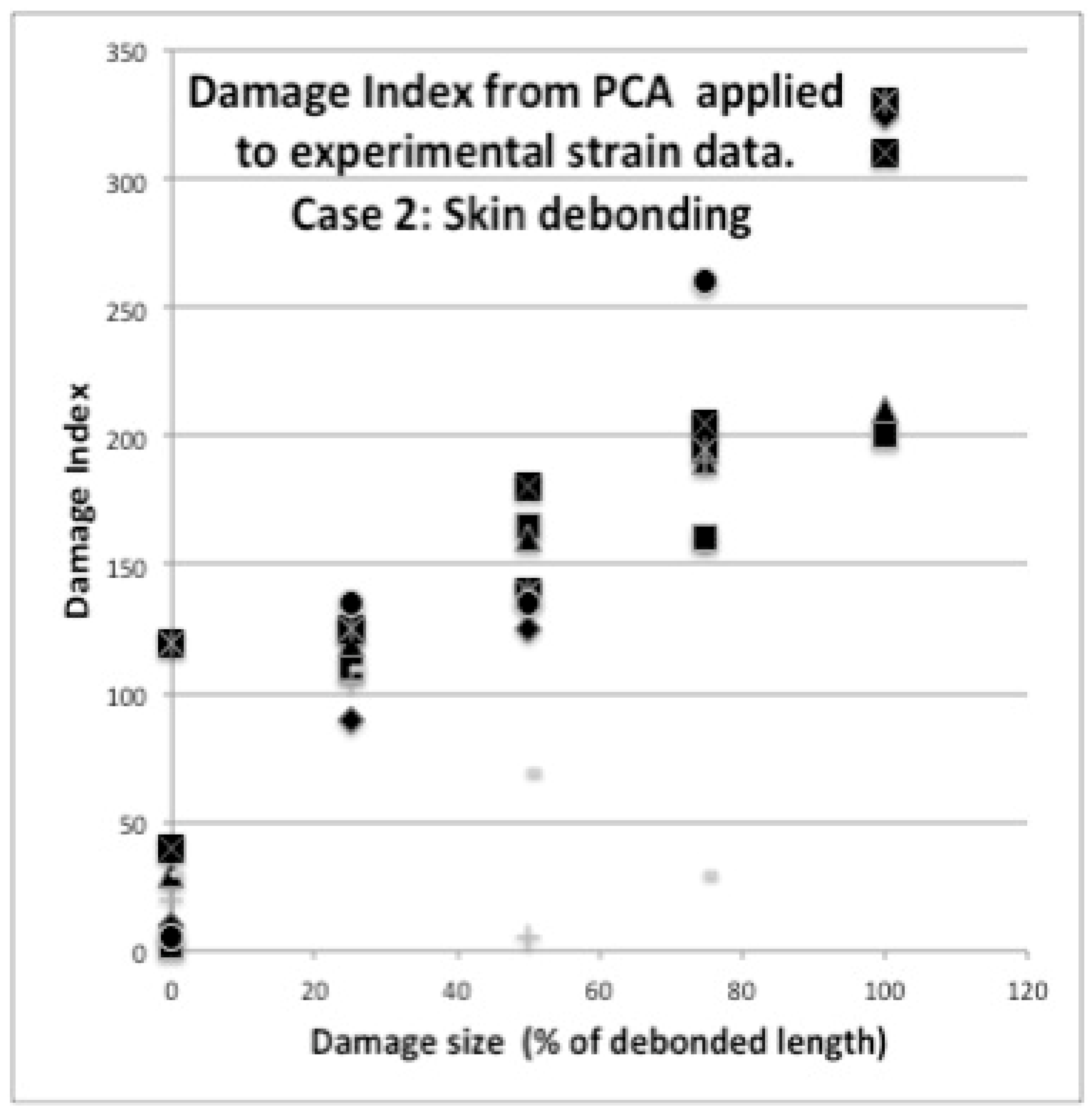
An application example of this methodology on a real structure—the fuselage of an unmanned aerial vehicle (UAV), 3 m long, which is detailed in [10]. Figure 7 shows the fuselage mounted in a test rig with an optical fiber bonded in four loops on its surface. Figure 8 depicts the measured strains for pristine and damaged structures, where the damage consists of partial debonding between the two fuselage skins. Only for the case of full debonding are differences visible. Also shown in Figure 9 is the calculated Damage Index after progressive damage. Notably, for this type of damage, when the size exceeds 25%, detection is unambiguous.

4.2. MAPOD and Digital Twins

The previously described algorithm requires that the physical structure is already built, that sensors are installed, and that a large number of load tests are conducted—procedures that can be costly and time-consuming. Simulation can significantly reduce these costs by enabling virtual experiments in which load conditions, sensor number and placement, and damage size are varied. These virtual tests can be used to compute Model-Assisted Probability of Detection (MAPOD), a process that is now common in non-destructive testing (NDT) procedures.

Prior to the availability of the physical structure, the process can be simulated as follows (Figure 10):

• Define the number and positions of sensors on the structure.
• Develop a conventional Finite Element Model (FEM) of the structure.
• Introduce a load case and compute the strain distribution throughout the structure.
• Extract the strain values at the sensor locations from the FEM results.
• Add random noise to these strain values to simulate the data collected from the pristine structure (corresponding to point 2 of the experimental algorithm). This is a critical step for the validity of the simulation; the sources of noise include the resolution of the strain reading equipment, among others.
• Introduce a simulated damage in the FEM—for instance, by disconnecting certain elements at nodes where a crack is assumed to exist. Rerun the FEM analysis, and obtain a new set of strain data, again adding noise.
• Apply the chosen algorithm (either PCA or ANN) to compare the pre- and post-damage datasets, as outlined in points 4 and 5 of the experimental procedure.

The results from applying the PCA algorithm to data generated by the FEM model of the aforementioned structure are detailed in [10]. The predicted detectability of damage was found to be similar to the results obtained from real experimental tests.

4.3. Supervised Learning. Algorithms Based on Artificial Neural Networks (ANNs)

A long list of articles dealing with SHM and machine learning fits within this category, and among them, those papers using images as datasets—obtained by non-contact sensors such as cameras or drones—and CNNs (Convolutional Neural Networks) as algorithms to extract the information play a dominant role. Ref. [19] presents a thorough review of nearly one hundred references, mostly in the field of civil infrastructure. As mentioned before, the larger the number of datasets to train the NN, the better the predictions are, and handling images facilitates this purpose very well. Very few cases have been studied in real in-field applications; up to now, most of the analyses have been performed on laboratory experiments. The availability of data from the pristine and damaged structures to train the network is a major bottleneck. Papers working on data coming from fiber optic sensors, and processed by ANN, are listed as Refs [20,21,22,23,24,25,26,27,28,29,30,31]. The group at Princeton has worked on a real structure, a pedestrian bridge located at that university, producing several papers related to NN, but not for damage detection. Rather, they aim to correct the environmental effects on the sensors.

With the digital twin of the UAV fuselage mentioned previously, an LSTM network (Long Short-Term Memory) was trained and validated for one undamaged and two progressive damage cases. Training was completed with 400 simulated load cases, and validation was performed on 80 cases. An accuracy of 96% was achieved, but when real strain data obtained from the experiment were used for the validation, this accuracy dropped to 81%. This is still a fairly high value, but it could be improved if better agreement between the FEM model and the real structure were achieved, and with a higher amount of training data. Full details are given in [14].

4.4. Comparison of Algorithms for Damage Detection (PCA vs. ANN)

Both PCA and ANN implementations are available through basic software tools such as MATLAB 2023b. The process involves preparing the strain data arrays—before and after damage—and then selecting the appropriate parameters in the corresponding tool.

4.4.1. Benefits of PCA (Principal Component Analysis)

Simplicity and Robustness

PCA is a straightforward and robust multivariate analysis technique that requires only the strain data from the undamaged structure as input (collected over multiple tests for statistical significance) and the strain data from the damaged structure.

Damage Index

The output is a single scalar value—the Damage Index (DI)—which quantifies how well the new strain data fit within the distribution of the pristine data. The DI increases with damage size, although the type of damage may also affect its value. (For example, delaminations in composite laminates are challenging to detect unless they induce local buckling because the associated strain changes are very small.)

Limitations

PCA does not provide information about the damage type or its exact location within the structure; it only indicates damage occurrence (corresponding to Level 1 of SHM). Subsequent analysis of the strain distribution is required to localize the damage.

4.4.2. Benefits of ANN (Artificial Neural Networks)

Data Requirements

ANN requires a large training dataset encompassing not only cases from the undamaged structure but also various damage cases and types anticipated during operation. This necessitates the existence of a numerical model of the structure to simulate both undamaged and damaged conditions.

Sensitivity and Specificity

Once adequately trained, ANNs can be more sensitive than PCA in detecting damage, provided that the damage type during the test is consistent with that used during training.

Output Information

In addition to indicating damage occurrence, ANN can provide information regarding the damage type and severity (aligned with Level 3 of SHM), but only if the particular damage type was included in the training set.

Potential Drawback

If an encountered damage type was not part of the training dataset, the ANN may yield inconclusive results.

5. Conclusions

Fiber optic sensors for strain measurements have achieved a high degree of maturity, both for point sensing and for distributed sensing, and they are used for a large variety of industrial applications. But they can measure only strain and temperature, so information about damage has to be derived from these measurements.

For the case of damage crossing the optical fiber path, there will be a big change in the strain reading, specifically at this point, so there is no need for further analysis. Damage is easily located with distributed fiber optic sensing. Many applications have already been reported in the literature; again, the approach can be considered mature.

For the more general case, when damage happens somewhere in the structure, the changes in the strain field are very mild, and there is a need for algorithms to compare the strain dataset before and after damage. Machine learning offers tools to perform this comparison, but these tools have to be carefully selected, and still, the damage detectability needs to be improved. Tools based on the unsupervised learning mode look easier to apply, as they only need data from the pristine structure and the strain dataset for the current condition. It must be pointed out that external loads and environmental conditions need to be identical during both strain readings.

For the supervised learning mode, datasets from the undamaged and damaged structures are needed to train the ANN, with different kinds of damage identified by labels. This is an important limitation when using the physical structure, but such datasets may be obtained from a digital twin, which works adequately, if properly executed.

Nevertheless, for both supervised and unsupervised modes, there is a need for further research before the method can be used outside laboratory test conditions. Temperature has a strong influence on the data obtained from the fiber optic sensors, so it may disturb the strain measurements if it is not adequately compensated.