Inverse Design of Plasmonic Nanostructures Using Machine Learning for Optimized Prediction of Physical Parameters

Abstract

Plasmonic nanostructures have been widely studied for their unique optical properties, which are useful in sensing, photonics, and energy. However, the efficient design of these structures, considering the complex relationship between geometry, material, and optical response, remains a challenge. In this study, we propose a machine learning-based approach to address the inverse design problem in nanostructures, using data generated by numerical simulations via the Finite Element Method (FEM). We used a dataset of over 140,000 entries to train the regression models CatBoost, Random Forest, and Extra Trees, capable of predicting physical parameters, such as the radius of the nanocylinder, based on the simulated optical response. The CatBoost model achieved the best performance, with a Mean Absolute Error below 0.3 nm on unseen data. In parallel, we applied a direct design approach to experimental data of metallic nanoparticles, focusing on the optical absorption prediction from particle size. In this case, Random Forest presented the best performance, with a lower risk of overfitting. The results indicate that machine learning models are promising tools for optimizing the design and characterization of plasmonic nanostructures, thus reducing the need for costly experimental techniques.

1. Introduction

Plasmonic nanostructures have attracted significant attention due to their unique ability to manipulate light at the nanoscale [1]. Their distinct properties arise from the high surface/volume ratio and the quantum effects that emerge at this scale [2].

Advances in nanophotonics have led to remarkable breakthroughs, such as the diffraction limit, with promising applications in optical sensors [3], photodetectors [4], and communication devices [5,6].

Considering the increasing focus on miniaturization at the nanoscale, the study of nanostructures has been extensively investigated for space applications [7,8,9,10,11]. The reduction in the size and mass of components in orbit simplifies designs and may enable more efficient and cost-effective space missions. The main applications include lightweight structures, damage-tolerant systems, nanocoatings, adhesives, and thermal protection materials, significantly enhancing mission efficiency and effectiveness [12]. Nanostructures, such as quantum dots and various nanomaterials, are used in nanomedicine, diagnostics, and nanotheranostics [13,14]. In recent years, the nanotechnology field has witnessed significant advancements in the synthesis of nanomaterials tailored for applications in medical diagnostics [15]. Nanostructured materials are also essential for improving the efficiency of solar cells, as they optimize light absorption and facilitate charge carrier mobility, thus maximizing energy conversion and device performance [16].

Nanostructured materials are also widely investigated in the field of sensors [17,18]. Another emerging area is green hydrogen production and storage, a sustainable alternative for clean energy generation. Nanostructures play a key role in this field, being applied in electrocatalytic and photocatalytic hydrogen production, advancements in hydrogen storage materials, and broader energy storage applications, including batteries and supercapacitors [19]. For these and other applications, the on-demand design of plasmonic nanostructures is fundamental.

The optical response of nanostructures strongly depends on their geometry and the materials employed, such as gold and silver, which exhibit different plasmonic properties at visible and infrared wavelengths [20,21]. The plasmonic resonance wavelength depends on the nanostructure’s shape, size, and material [22].

However, the efficient design of nanostructures that optimize these properties remains a challenge. Characterizing these materials is essential to predict and control their optical, photothermal, and mechanical properties. Nevertheless, conventional characterization techniques present significant limitations, such as cost and infrastructure. SEM and TEM equipment require high investment and specialized infrastructure. Additionally, their field of view may not fully reflect the nanoparticles’ overall size and distribution [23]; regarding time and complexity, measurements and analyses can be time-consuming and require specialized training [24]. The limited availability of such equipment in many institutions and companies results in long waiting times for analyses, which hinders the progress of studies in smaller research groups.

Computational tools enable the optimization of these nanomaterials as a starting point for obtaining their design, which can be validated later by experimental data [25]. Computational models based on the Finite Element Method (FEM) and the Finite-Difference Time-Domain Method (FDTD) tend to be significantly time-consuming and resource-intensive, in addition to requiring substantial memory [26]. Each unit of the geometric mesh is calculated based on Maxwell’s equations and on environmental conditions that depend on boundary conditions. The runtime of these simulations varies significantly depending on the complexity of the simulated structure, the applied boundary conditions, and the defined level of accuracy, especially regarding mesh refinement [27].

The use of machine learning (ML) techniques in the inverse design of nanophotonic structures has emerged as a promising approach to overcome the challenges associated with the complex relationship between geometry and optical response. Due to the strong dependence of electromagnetic properties on structural geometry, and the non-intuitive nature of this relationship, traditional methods are limited in both efficiency and scalability. In contrast, ML algorithms have demonstrated the ability to model such behaviors with high accuracy and significantly reduced inference times, enabling the creation of on-demand geometries optimized for specific functionalities [28]. This approach accelerates the design process and enhances the optimization of nanostructures for various applications. Once trained, ML algorithms can process any data within the designed scope while maintaining relatively stable performance regardless of the complexity and volume of the data. In contrast, traditional simulation software displays a significant increase in processing time as problem complexity grows [29]. The methodology proposed here will enable the efficient and targeted design of nanostructures with specific optical properties. For example, it will be possible to determine appropriate dimensions and materials to achieve absorption in specific electromagnetic spectrum ranges.

The work presented by Acharige et al. [28] investigated strategies to enhance the efficiency of inverse design in nanophotonic structures, with a focus on predicting optical responses outside the training range. The results showed that different approaches exhibit varying performance in spectral interpolation and extrapolation tasks. These findings underscore the importance of selecting appropriate methods based on the specific goals of inverse design, particularly in scenarios where data are limited.

A hybrid inverse design approach was also proposed to optimize plasmonic structures used in localized structured illumination microscopy. The methodology combines optimization algorithms and electromagnetic simulations to design emitters that enhance optical resolution. The results demonstrate significant improvements in both performance and the spatial control of light at the nanoscale [30].

A related study on plasmonic sensors presents the development of an optical hydrogen sensor with sensitivity in the parts-per-billion (ppb) range. Using a particle swarm optimization (PSO) algorithm, the authors inversely designed a plasmonic metasurface composed of a periodic array of palladium (Pd) nanoparticles. The study highlights the potential of inverse design to significantly enhance the sensitivity of plasmonic sensors for ultra-sensitive optical gas detection applications [31].

Liang et al. [32] proposed an inverse design strategy for photonic–plasmonic devices with a focus on light superfocusing. The authors developed a physics-guided, two-stage neural network incorporating enhanced coupled-mode theory to guide the learning process. Additionally, an approach for designing plasmonic nanotweezers using topology optimization was presented. The authors employed adjoint sensitivity analysis to engineer nanostructures that maximize electric field confinement, which is essential for the efficient optical trapping of nanoparticles. This methodology enables the creation of non-intuitive geometries that overcome conventional design limitations, resulting in enhanced performance for nanoscale optical manipulation [33].

The present work focuses on the inverse design of plasmonic nanostructures, aiming to optimize the accurate prediction of physical parameters of nanocylinders, radius/height, based on observable data, including material, wavelength, and scattering. Using advanced simulations based on the FEM, we collected a robust dataset to train machine learning models such as Random Forest, CatBoost, and Extra Trees. In addition, we also trained the models using experimental data from gold nanoparticles suspended in a colloidal solution; however, in this case, we focused on direct design. The proposed method minimizes the need for robust and financially inaccessible equipment, which may hinder nanoparticle characterization. This makes the process significantly more accessible, thus reducing costs and increasing efficiency in the characterization and optimization of these nanostructures.

2. Theoretical Framework

Random Forest, developed by [34], is a supervised machine learning method used for regression and classification that combines the output of multiple Decision Tree models to improve the prediction accuracy. This method is based on the bagging approach for ensemble learning, in which multiple simpler models (weak learners) are built and combined to obtain a more robust model (strong learner). In the Random Forest, the weak learners are Decision Trees, which are hierarchically supervised learning models formed by nodes that apply tests to the data to increase the purity of each node, generally based on entropy.

The Random Forest trains several Decision Trees independently, using random subsets of the training samples and attributes, and then, it aggregates the results to generate a more reliable prediction. The final output is constructed from the average or vote of the predictions made by each individual Decision Tree. This approach reduces the variance of the estimation and improves the generalization capacity of the model, making it more robust and with a lower risk of overfitting.

Extra Trees (or Extremely Randomized Trees) [35] is also a supervised machine learning method used for regression and classification based on bagging. However, this method proposes an improvement in the process of tree construction. While Random Forest randomly selects a subset of attributes in each node, Extra Trees selects a random split point for the features. In each node, instead of calculating the best split of the data based on some criterion such as entropy, Extra Trees defines these split points completely randomly. This process makes training faster, since the splits are chosen randomly instead of being calculated deterministically. In addition, Extra Trees tends to be more robust to noise due to the greater randomness during training, making it more efficient in certain scenarios where Random Forest is not able to overcome them.

CatBoost (Categorical Boosting) [36] is a supervised learning technique used for regression and classification based on the Boosting approach using Decision Trees. Boosting is an ensemble learning approach in which several learning algorithms (weak learners) are used sequentially to generate the final model (weak learners). Each individual model learns from the errors of previous models to make better predictions in the future; that is, the errors are used to train new learning models, reducing the bias of the output.

CatBoost uses Binary Decision Trees as weak learners and its main innovations in relation to other Boosting approaches are Ordered Boosting and Symmetric Trees. While other Boosting algorithms have overlap between the training data used to build the base models and the data used to calculate the gradients, CatBoost performs a random permutation of the data and uses only the previous data of each example in the permutation for training. Furthermore, CatBoost builds Balanced (or Symmetric) Trees, in which all nodes at the same level share the same decision rule, unlike traditional methods that build trees that can be asymmetric. These characteristics lead to faster execution and reduce the probability of overfitting.

3. Materials and Methods

3.1. Theoretical Dataset

The simulations carried out in this work employed the finite element method (FEM), implemented using COMSOL Multiphysics^® (version 6.2). Initially, we defined the geometry of the problem, consisting of nanocylinders fabricated from different materials: gold, silver, and copper. The nanocylinder was placed on a silica (SiO₂) base to more accurately reflect practical experimental settings, which enabled the consideration of changes in the plasmonic resonance caused by the substrate. The simulations focused on perfect cylindrical shapes without any structural inconsistencies to create a clear and systematic dataset for assessing regression-driven inverse design. While geometric flaws and irregularities often occur in nanostructures made in experiments, omitting them at this phase facilitated results that were easier to understand and replicate.

We parameterized each nanocylinder according to variables of interest, such as height, radius, and incident wavelength. These variables were systematically adjusted to generate a comprehensive dataset, which enabled us to carry out a detailed study of the optical response of the nanostructures.

Within the COMSOL environment, the simulations considered specific boundary conditions, such as incident electromagnetic field conditions, and the use of refined meshes to ensure greater accuracy in the results.

We simulated the interaction of light with the nanocylinders over a wavelength range spanning from the visible to the near-infrared region, from 400 nm to 1200 nm, to characterize the scattering and absorption parameters of the structures. We used three types of materials in the simulation: gold (Au), silver (Ag), and copper (Cu). For each set of geometric and material parameters, we calculated its corresponding scattering spectrum and stored them along with its respective input variables in a database containing approximately 140,000 data points. Thus, we used the generated data in the subsequent machine learning stage to build an inverse design model for predicting the geometric parameters of the nanostructures based on the simulated optical responses.

In this study, we systematically varied the geometric parameters of the nanostructure height (h) and radius (a) to generate a comprehensive dataset. We adjusted the height (h) within a 100 nm to 300 nm range, with increments of 10 nm, and the radius (a) within a 50 nm to 150 nm range for each fixed height value, with the same 10 nm increments. With these data, we obtained a dataset of more than 140,000 data points.

To achieve reliability and consistency in the created dataset, the simulations were executed in a methodical manner by changing one parameter at a time—either the radius, height, or wavelength—while keeping the other parameters constant within specified limits. Each combination set was simulated under uniform physical boundary conditions, utilizing a silica (SiO₂) substrate and an appropriate mesh refinement method to accurately represent near-field interactions around the nanostructure. The selection of materials (Au, Ag, Cu) and the wavelength range from 400 nm to 1200 nm was informed by standard plasmonic characteristics in the visible to near-infrared spectrum. These managed parameters facilitated the development of an organized and equitable dataset for training and assessing the regression models.

3.2. Dataset Experimental

We produced silver nanostructures with varying average sizes and used them in the composition of the dataset. The sizes were experimentally determined through complementary techniques of spectroscopy and Transmission Electron Microscopy (TEM). Spectroscopy enabled the analysis of optical properties and the inference of information related to the average particle size, while TEM provided direct measurements related to the morphology, dimensions, and distribution of the nanostructures. Combining these two techniques resulted in the precise characterization of the nanostructures, ensuring a robust and reliable analysis for predictive model development. We obtained absorption results using UV–visible (UV–Vis) optical spectroscopy, in which light is directed onto the sample containing the nanostructures, and in measuring the intensity of incident and transmitted light through the sample, the acquisition spectrum is determined, highlighting the wavelengths at which maximum absorption occurs.

A dataset comprising the average size of nanoparticles, a wavelength sweep ranging from 300 nm to 1000 nm, and the corresponding absorption spectra was successfully obtained, yielding approximately 13,000 data points.

3.3. Regression

The method we implemented in this work employs regression algorithms to predict the structural parameters of cylindrical nanostructures that yield specific desired responses. The machine learning-based approach uses a dataset generated via the FEM and evaluates the performance of the regression models under different training/test split ratios. Initially, the dataset is loaded, and a fixed subset is separated for final validation, defined by the following conditions:

• Height = 300.0 nm;
• Wavelength ($\lambda$) = 1184.0 nm;
• Material = copper (Cu).

This reserved set is not used during training or validation and serves exclusively for the final evaluation of the model, thus representing a test phase. Additionally, we included a radius of 75 nm in the separated subset, which does not appear at any other height in the dataset. The goal is to assess whether the regression algorithms generalize well to unseen data.

Later, the code iterates on the remaining data over different training ratios of 30%, 40%, 50%, 60%, 70%, and 80%. We split the data into three sets for each ratio: training, validation, and testing. The PyCaret environment was configured within each data split for regression tasks, using version 3.3.2. Three candidate models were trained separately: CatBoost (version 1.2.8), Random Forest and Extra Trees (implemented via scikit-learn version 1.4.2).

The code generates predictions for each model on the training, validation, and test sets, and then, it calculates various performance metrics, such as the Mean Absolute Error (MAE), Mean Squared Error (MSE), and Coefficient of Determination (R²). By comparing the metrics between the training and validation sets, the algorithm allows the identification of signs of overfitting, verifying whether there are significant discrepancies between the errors or if R² presents high values accompanied by serious errors.

In summary, the code workflow is as follows:

• It loads the data and separates a fixed set for the final test phase.
• For each training proportion, from 40% to 80%, the remaining data are equally divided between test and validation sets.
• PyCaret is configured for regression, and candidate models are trained.
• Performance metrics MAE, MSE, and R² are calculated for the training, validation, and test sets, thus enabling the analysis of possible overfitting.
• Graphs illustrating model performance are generated and saved.
• The best model is selected based on the lowest MAE from the internal validation set, and a final evaluation is performed using the reserved set.

This approach enables both a quantitative comparison of the models and a detailed visual analysis, thus ensuring the selection of the model with the best generalization capacity for new data.

All regression models were created using the PyCaret library through the create_model function, which utilizes the standard hyperparameters from the foundational libraries, like scikit-learn for Random Forest and Extra Trees, as well as CatBoost’s original configurations for gradient boosting. At this point, no adjustments to hyperparameters were made, since the main objective was to evaluate the models under uniform and standardized circumstances.

Among the various options, CatBoost is notable for its use of integrated regularization methods, which consist of L2 regularization (l2_leaf_reg = $3.0$), Ordered Boosting, and Symmetric Trees. These characteristics aid in mitigating overfitting by promoting a more cautious approach to learning. In contrast, Random Forest and Extra Trees were utilized without specific regularization or limitations on depth, resulting in significantly low training errors but also creating larger discrepancies between training and validation outcomes.

These design choices are reflected in the performance metrics discussed in the results and reinforce how differences in model architecture and regularization strategies can significantly influence generalization, especially in inverse modeling tasks with limited data.

Table 1. Default hyperparameters used by each regression model as implemented via PyCaret.

Model	n_Estimators	Max_Depth	Learning_Rate	L2 Reg.	Strategy
catboost	1000	6	0.03	3.0	Ordered Boosting, Symmetric Trees
rf	100	None	–	–	Bootstrap + Gini/MSE
et	100	None	–	–	Totally Random Splits

presents the main default hyperparameters adopted for each model, such as the number of estimators, maximum tree depth, learning rate (when applicable), and regularization methods.

The CatBoost model employs Ordered Boosting and Symmetric Trees, offering robustness against overfitting and efficient handling of structured data. Random Forest follows scikit-learn defaults, using bootstrap aggregation with deterministic splits. Extra Trees introduces randomness by selecting split points randomly, which can enhance generalization but may reduce stability in some cases.

Regarding the experimental data, we used the algorithms to predict absorption based on the nanoparticle size. Due to the limited dataset, which contains only about 13,000 points compared to the theoretical data obtained through FEM, there is a restriction on the number of samples available for model training.

The procedure is the same as that used for inverse design but with absorption as the new output. Thus, the fixed subset reserved for final validation is defined for the average size of 7.5332077 nm.

4. Results

4.1. Inverse Design Using Theoretical Data

To verify whether the regressors were accurately generalizing the models, we performed a comparison of the MAE metric obtained after validation by analyzing the training, validation, and test values. The graphs presented in Figure 1 illustrate the variation in the MAE metric as a function of the training data proportion, Training Ratio, for three different models: CatBoost, Extra Trees, and Random Forest. From this figure, we observe that the MAE metric changes as the amount of training data increases, reflecting the impact of the Training Ratio on the model’s generalization. In general, we expect that the error decreases as more training data are used since the model has more information to learn from. The three graphs display that the MAE for the training set is lower compared to the test and validation sets, which is an expected behavior. For the Extra Trees and Random Forest models, the MAE values for the training, test, and validation sets are considerably lower compared to CatBoost; however, the ratio between training/validation and training/test is significantly lower for the CatBoost model.

Next, we highlight some considerations regarding overfitting. The Extra Trees regressor achieves the best performance in terms of MAE on both test and validation sets, reaching near-zero error on the training set. This model presents extremely low training errors, indicating a strong capacity to fit the training data, which is a clear sign of potential overfitting. For example, at a Training Ratio of $0.4$, the training MAE is $0.04$, while the test MAE is $0.96$, with a gap of approximately $0.92$. Although the model clearly overfits the training data, it still outperforms the others on the test and validation sets, which suggests that, despite the strong overfitting in terms of the MAE gap, Extra Trees does not suffer from a loss of generalization for this test/validation set.

Random Forest ranks second, with MAEs lower than those of CatBoost but slightly higher than those of Extra Trees. Random Forest also presents low training MAEs, around $0.4$, and slightly higher test and validation MAEs, above $0.8$ in some cases, which characterizes a relevant gap. Compared to Extra Trees, the overfitting gap is slightly smaller but still considerable.

CatBoost presents less difference between the training MAE and test/validation MAE, while presenting final MAEs higher than those of the the others. This regressor is the most stable in the sense of having a smaller gap, difference, and ratio between the training and test MAE, thus indicating a lower risk of overfitting. For example, at a Training Ratio of $0.4$, the training MAE is $1.76$, while the test/validation MAEs are around $1.84$–$1.86$, which results in a smaller gap of $0.09$.

Table 2. Regression metric results for different models and training data proportions. Table 2 presents the coefficients of determination (R²), the Mean Absolute Errors for the training, test, and validation sets, as well as the ratio between the Mean Errors (MAE ratio). The evaluated models include CatBoost, Random Forest (rf), and Extra Trees (et).

Training Ratio	Model	r2 Training	Mae Training	r2 Test	Mae Test	r2 Valid	Mae Valid	Mae Ratio
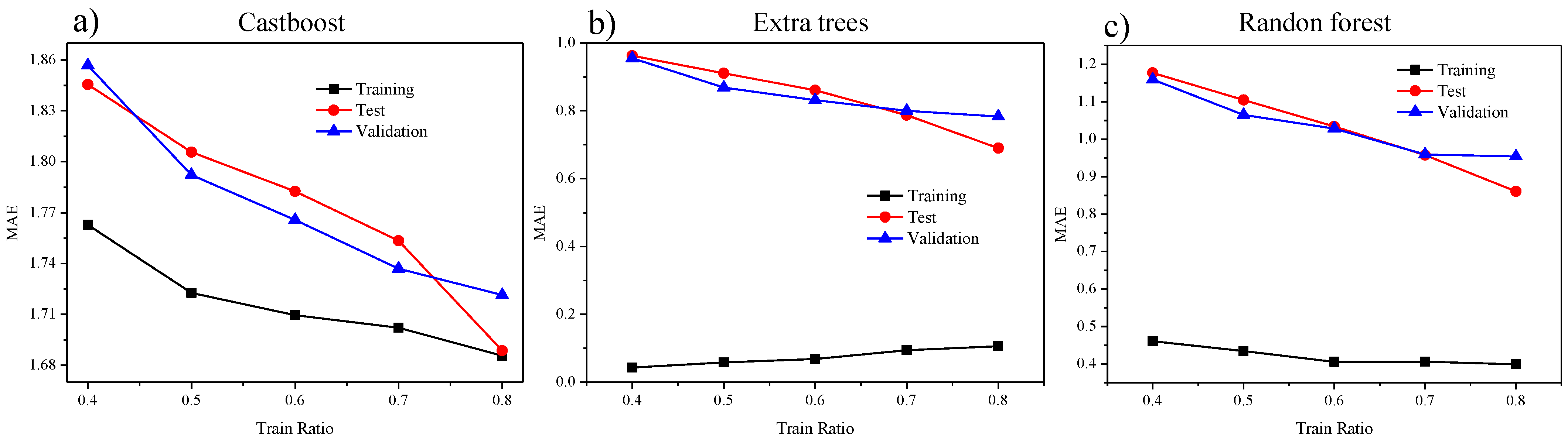
0.4	catboost	0.984	1.763	0.980	1.845	0.981	1.857	1.053
0.4	rf	0.996	0.460	0.978	1.177	0.980	1.159	2.518
0.4	et	0.998	0.043	0.978	0.962	0.979	0.955	22.212
0.5	catboost	0.984	1.723	0.979	1.806	0.982	1.792	1.040
0.5	rf	0.996	0.434	0.977	1.104	0.981	1.065	2.451
0.5	et	0.998	0.058	0.976	0.911	0.979	0.868	14.929
0.6	catboost	0.983	1.710	0.981	1.783	0.981	1.766	1.033
0.6	rf	0.996	0.406	0.978	1.034	0.978	1.028	2.534
0.6	et	0.998	0.069	0.975	0.861	0.977	0.832	12.114
0.7	catboost	0.983	1.702	0.982	1.753	0.983	1.737	1.020
0.7	rf	0.995	0.406	0.980	0.957	0.981	0.959	2.361
0.7	et	0.997	0.094	0.977	0.787	0.977	0.800	8.493
0.8	catboost	0.983	1.686	0.985	1.689	0.983	1.721	1.021
0.8	rf	0.994	0.399	0.984	0.861	0.980	0.954	2.389
0.8	et	0.996	0.106	0.981	0.690	0.975	0.783	7.374

presents the regression metrics for the three machine learning models under different training data proportions, with the training ratio varying from 0.4 to 0.8 (i.e., 40% to 80% of the dataset used for training). CatBoost maintains a relatively stable MAE ratio close to 1, indicating good generalization and low overfitting, regardless of the training proportion. Random Forest exhibits MAE ratios ranging from approximately 2.3 to 2.6, suggesting moderate overfitting. Extra Trees presents the highest values, exceeding 22 in some cases, which indicates strong overfitting. Notably, the MAE ratio tends to decrease as the training ratio increases, due to the larger amount of training data and reduced validation set.

To gain a clearer picture of how each algorithm generalizes to different plasmonic materials, we calculated the MAE ratio (the validation MAE divided by the training MAE) for each model, maintaining a training ratio of 0.7. The information is shown in

Table 3. MAE ratio for each model across the three materials, considering a training ratio of 0.7.

Material	Model	Mae Ratio
Gold	catBoost	1.005
Gold	rf	2.293
Gold	et	8.199
Silver	catBoost	1.009
Silver	rf	2.292
Silver	et	8.069
Copper	catBoost	1.020
Copper	rf	2.361
Copper	et	8.493

, which highlights that CatBoost consistently exhibits minimal error amplification on gold, silver, and copper, while Random Forest and Extra Trees exhibit notably larger ratios, suggesting a tendency toward overfitting.

Figure 2, Figure 3 and Figure 4 show the quantile–quantile (Q–Q) plots, which compare the distribution of the model residuals to that of a normal distribution. These plots help assess whether the residuals follow a roughly normal pattern by placing the ordered residuals against the theoretical quantiles. When the points closely follow the reference line, it suggests that the residuals are approximately normally distributed—a desirable property in regression analysis.

The distribution of residuals can influence the quality of the model, allowing for the assessment of whether overfitting occurs, for example. In Figure 2, we present the data related to the CatBoost model, thus demonstrating a consistency of points along the fitting line when varying the training data, which indicates that the residuals adhere well to normality. In contrast, in Figure 3, regarding the Random Forest model, the residuals are very flattened, i.e., concentrated around zero, so they do not follow the expected distribution. This may be a strong indication that the model underestimates the variability of the residuals, thus suggesting that it may be masking normality by producing predictions that are too close. We observe a similar behavior for the Extra Trees model in Figure 4, where the residuals are concentrated at zero. In the case of the 0.5 training split, the points are flattened, while for other splits, the residuals present deviations, which may indicate that the model does not generalize well to unseen data.

Among the three models, CatBoost appears to be the most stable, presenting well-distributed residuals with better adherence to normality. This behavior is consistent across all splits. In comparison, Random Forest and Extra Trees fail to model or capture the distribution of residuals well, possibly due to overfitting. The dispersion of the points is quite small, which indicates excessive smoothing in the predictions.

The residual plot is a useful tool for assessing the regression model’s performance, as it provides a qualitative evaluation of the model’s fit. The residuals represent the difference between the real values and the predicted values. When there is a random dispersion of the residuals around zero, it indicates that the model has effectively captured the underlying patterns in the data. However, if the residuals present a specific pattern, it may indicate an ineffective capture of the data [37].

In Figure 5a, we observe that the residuals are randomly distributed around zero, such that there is no obvious pattern. Nevertheless, such dispersion is not uniform around the red line, zero, which indicates heteroscedasticity [38], which is a variation that depends on the predicted value. The model may not be accurately capturing some patterns in the data, as suggested by the curved trend of the points. On the other hand, due to the randomness of the dispersion, the model is learning the patterns, although it does not fit the data perfectly.

For the Extra Trees and Random Forest models shown in Figure 5b,c, the residuals are either very close to the zero line or positioned right on it, thus suggesting low variability in the errors. This behavior may be another indication of overfitting, as there is insignificant variation in the errors except for a few isolated outliers. Hence, the models do not capture the full complexity of the data.

The plots demonstrated in Figure 6 compare the prediction of the nanocylinder radius with the real value for the respective regression models and two training proportions: $0.3$, which is the smallest amount of training data; and $0.7$, a Training Ratio that usually tends to provide better generalization. The red line represents the ideal fit $y=x$, and the blue dots correspond to the model predictions as a function of the real values. The radius of 75 nm, which was not seen during training, testing, or validation, is highlighted with a red arrow, indicating a crucial point for assessing the generalization capability of the models.

In general, the three models appear to fit well with the radius values commonly used and present in the dataset. Nevertheless, when analyzing the 75 nm radius in isolation—which is a data point entirely new to the models—there was a slight error in its generalization, which is evidenced mainly in the Random Forest and Extra Trees models.

The CatBoost model, presented in Figure 6a,d,e, demonstrates the best performance in generalizing to the 75 nm radius, once it produces significantly lower errors when compared to the other models, as indicated in

Table 4. Comparison of the prediction of the 75 nm radius between the models.

Modelo	Training Ratio	Predição Para 75 nm	Erro Absoluto (nm)
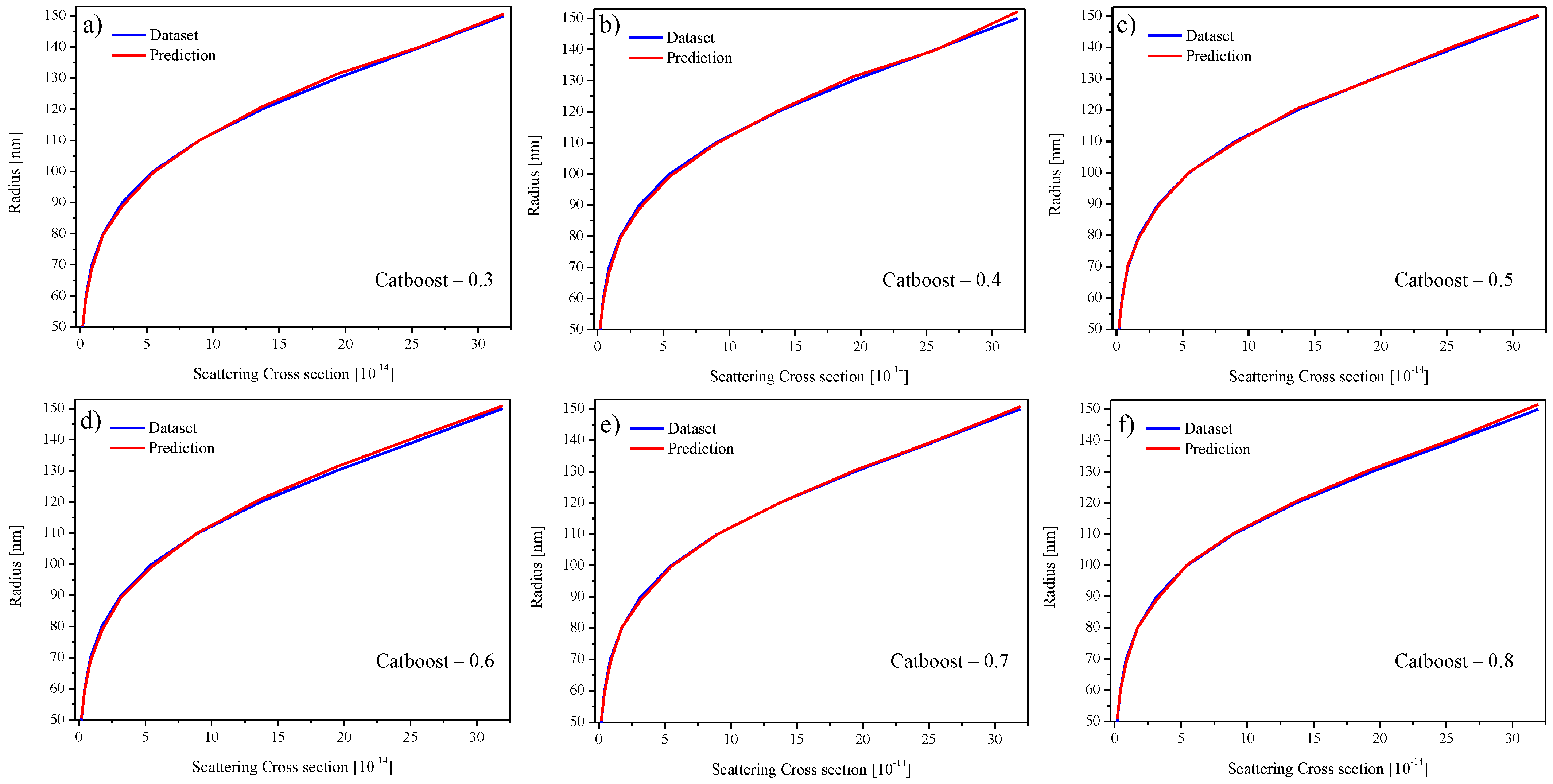
CatBoost	0.3	74.63	0.37
CatBoost	0.7	74.75	0.25
Extra Trees	0.3	76.80	1.80
Extra Trees	0.7	78.00	3.00
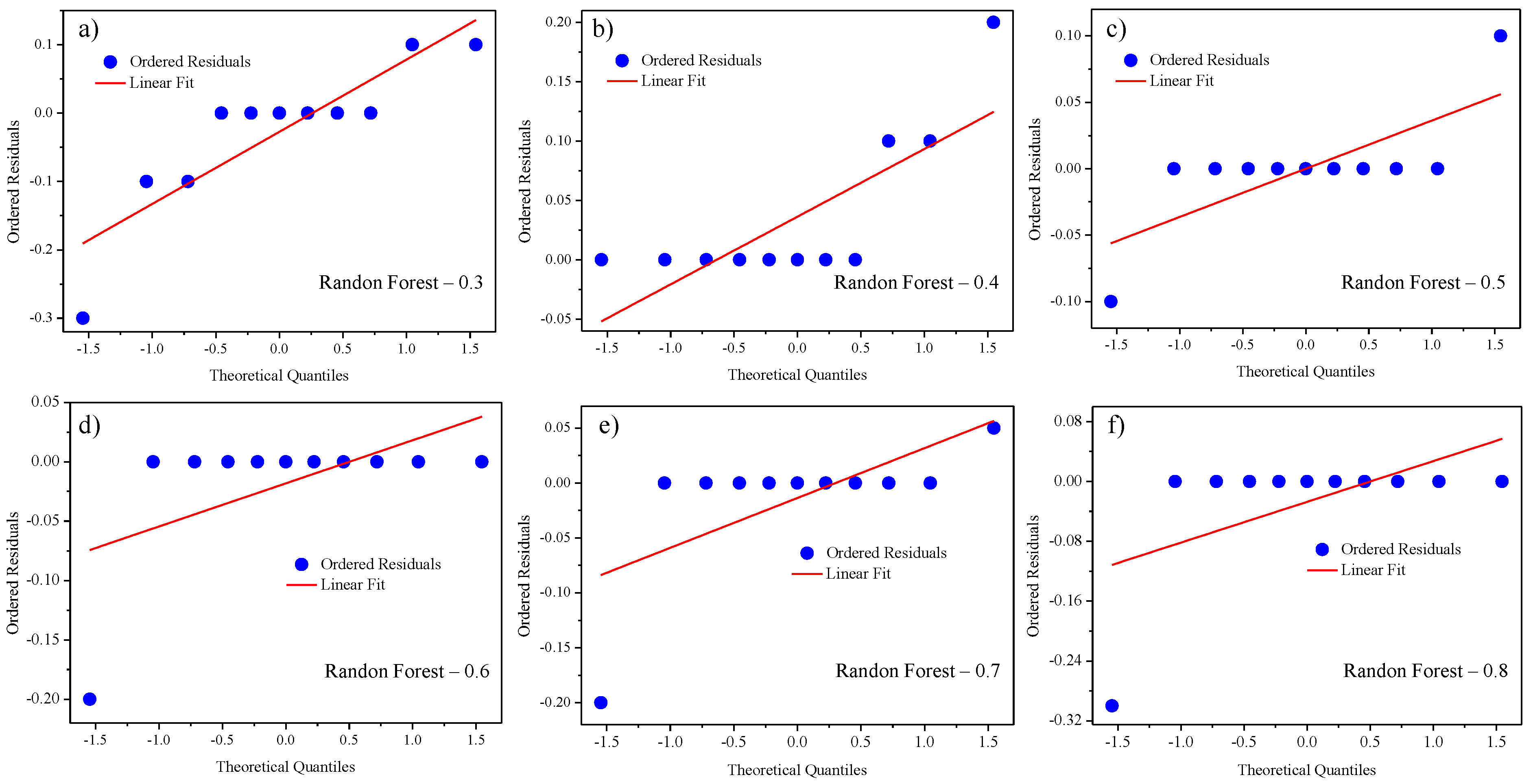
Random Forest	0.3	77.40	2.40
Random Forest	0.7	78.00	3.00

. This table presents the exact predicted values for each model and the training ratios of 0.3 and 0.7, along with a comparison of the absolute errors. The Random Forest and Extra Trees models demonstrate a certain tendency to overestimate unseen data, especially when the Training Ratio is 0.7, which indicates that increasing the amount of training data does not improve extrapolation. In contrast, the CatBoost model reduced the error when we increased training data. Thus, we infer that CatBoost demonstrates better generalization to unseen data, whereas Random Forest and Extra Trees learn the training data well but have a reduced ability to predict new values.

Considering the discussions raised about the generalization of the models, the analyses we conducted indicate a consistent trend of better performance by the CatBoost model compared to the others. The results reveal that CatBoost presented the lowest absolute errors in predicting the 75 nm radius, a value not included in the training set. With a Training Ratio of 0.7, the absolute error was only 0.25 nm, which is significantly lower than that observed in the Extra Trees and Random Forest models, which in turn showed more substantial deviations, reaching up to 3 nm.

Furthermore, the residual and Q–Q plots highlight that CatBoost exhibits a more uniform error pattern without significant systematic deviations. In contrast, the Extra Trees and Random Forest models tend to overestimate the 75 nm radius, possibly due to overfitting or difficulties in extrapolation.

When evaluating the overall performance, it is evident that, although all models maintained a good linear fit for the data seen during training, CatBoost demonstrated a greater capacity to adapt to new values, making it the best choice for generalization and robustness in predicting the nanocylinder radius. Therefore, we used CatBoost to perform the final prediction of all radii as a function of one of the input variables, in this case, the Scattering Cross–Section. We chose this input variable based on feature importance, as the output variable demonstrated dependence on this input variable greater than the height, material, and wavelength.

Figure 7 displays the comparison between the real data and the predicted data for each of the training ratios. We observed that, regardless of the training percentage used, there is good agreement between the curves, thus demonstrating the model’s effectiveness in predicting the nanocylinder radius from the Scattering Cross-Section. It is noteworthy that, even when using only 50% of the data for training, we achieve a high-quality fit to the real values, as illustrated in Figure 7c. From this, we conclude that it is not necessary to use a large portion of the data to obtain a satisfactory prediction.

Although the 0.5 split already demonstrates excellent performance, the graphs indicate that smaller proportions, such as 0.3 (Figure 7a), also result in accurate predictions, with slight discrepancies. This suggests that CatBoost is capable of generalizing well, even with reduced training sets, which makes it an efficient option when data availability is limited.

Finally, when comparing higher training ratios, 0.6 and 0.8 to 0.5, we observed that the fit for 0.5 is slightly superior, thus indicating that increasing the amount of training data does not necessarily improve prediction and may even introduce small variations. Therefore, we conclude that this suggests that there is an optimal training point, and it indicates that adding more data does not result in significant performance gains for the model.

Among the three models evaluated, CatBoost consistently distinguished itself through its strong generalization capabilities, even with varying training and testing data splits. This was represented by the minimal difference in the Mean Absolute Error (MAE) observed between the training and validation datasets. This level of consistency can be attributed largely to CatBoost’s built-in features, such as L2 regularization (l2_leaf_reg) and its Ordered Boosting approach, which effectively mitigates overfitting by implementing more careful updates and utilizing data permutations during the training process.

On the other hand, Random Forest and Extra Trees were applied without restrictions concerning tree depth or any specific regularization measures. Although this approach resulted in significantly low errors within the training dataset, it simultaneously caused a notable rise in MAE within the validation dataset, indicative of overfitting. These findings underscore the importance of a model’s construction and regularization methods, as they can greatly influence performance, particularly in inverse design challenges where data availability is limited or the input space is intricate.

Recent developments in the field of nanophotonic inverse design have been concentrated on methods based on deep learning and optimization techniques. Research conducted by Acharige and Johlin [28] as well as Liang et al. [32] examined the use of physics-informed neural networks for spectral extrapolation and superfocusing. In addition, Wu et al. [30] integrated optimization with simulations to improve the resolution in structured illumination microscopy. Moreover, Nugroho et al. [31] highlighted the effectiveness of particle swarm optimization in the creation of highly sensitive plasmonic gas sensors.

Unlike these approaches, our study adopted classical tree-based regression models (CatBoost, Random Forest, Extra Trees) for inverse prediction. Despite their simplicity, these models achieved competitive accuracy and strong generalization across different materials, as shown by the MAE ratios close to 1.0 for CatBoost. This makes them particularly useful in data-limited or computationally constrained environments, offering a practical and interpretable alternative to more complex architectures.

4.2. Direct Design Using Experimental Data

Due to limitations in the quantity and resolution of the available experimental data, as well as the absence of accurately controlled geometric parameters for the nanoparticles, the application of inverse design techniques using experimental optical spectra was not feasible in the current study. While the direct prediction of absorption from particle size was implemented to demonstrate the model’s adaptability to real data, the inverse approach requires a more robust dataset with precise dimensional validation (e.g., through high-resolution TEM). Therefore, the inverse regression models were restricted to simulated data, where the input parameters are known and controlled. This constraint has been explicitly acknowledged and will be addressed in future work through the acquisition of expanded experimental datasets that support inverse predictive modeling.

The dataset containing the experimental data is limited compared to the dataset obtained from numerical simulation, with just over 13,000 points, which may impact the performance of the algorithms. The graphs presented in Figure 8, demonstrate the learning curves of each model based on the MAE metric obtained for each training proportion. In Figure 8a, the error for the CatBoost model’s training set is low and nearly constant, thus indicating that the model trained well, although exhibiting possible overfitting. The test curve, initially with a training proportion of 0.3, presents a high error, approximately 0.0028. As the training proportion increases, the error decreases significantly until it reaches a minimum of around 0.7, where it is approximately 0.0023. After 0.7, the error rises again, which may indicate the onset of overfitting or that the data used in the test set at this proportion did not adequately represent the general behavior of the entire dataset. The MAE presented by CatBoost reveals irregular behavior, initially close to the test set for smaller proportions, with a slight error decrease up to 0.5, thus increasing slightly up to the 0.7 proportion and dropping sharply at 0.8. Therefore, we conclude this indicates that 0.8 may be the ideal training proportion for this model in terms of generalization.

The Extra Trees model (Figure 8b) presents a considerable difference between the training set and the test and validation sets. This may be characterized as an indication of overfitting, given that the errors for the training set across all proportions are practically null. However, the learning curves for the training and validation sets follow a similar trend, thus indicating that a larger amount of data may help mitigate the generalization problem.

The Random Forest model, displayed in Figure 8c, appears to be the most suitable. The overall trend of the three curves is similar, presenting a progressive and smooth decrease as the amount of training data increases. Low training values demonstrate good learning capacity. Among the three models, Random Forest presents the lowest risk of overfitting, demonstrating stability and balance across the training, test, and validation sets.

This comparison among the three models demonstrates that the Random Forest model adapts better to datasets with more limited amounts of data, whereas for larger datasets, the CatBoost model is more suitable for generalization.

In evaluating the overall performance, Random Forest has the lowest error, followed by Extra Trees and CatBoost. The model that presents the lowest risk of overfitting is also Random Forest, with fewer differences between training and testing/validation. The irregularity of CatBoost may indicate instability in the results but not necessarily a high tendency toward overfitting. Although the CatBoost validation curve is irregular at lower proportions, there is a clear trend of error reduction as the amount of training data increases, especially at the highest proportion (0.8). This downward trend indicates that, despite the fluctuations, the model improved its generalization as it received more data. On the other hand, the extremely low training error of Extra Trees, combined with greater discrepancies in validation, indicates a higher risk of overfitting.

Figure 9 presents the Q–Q plot graphs of the models studied. The distribution of the residuals around normality follows a similar pattern for the three models; however, there is no normality of the residuals, especially about the extremes.

Figure 10 displays the prediction results compared with the real absorption values. Figure 10a–c represent the performance of each model for a training ratio of 0.7. For CatBoost, presented in Figure 10a, we observe a good adherence of the points to the fitting line, although slight and repeated variations occur along the line. Small pointwise deviations suggest localized errors but without major discrepancies. The points are uniformly distributed along the entire range, although certain irregularities occur between values of 0.2 and 0.3.

The Extra Trees model displayed in Figure 10b exhibits a consistent dispersion of points close to the ideal. Nevertheless, similar to the CatBoost model, it also presents irregularities in the 0.2 to 0.3 range. However, these irregular points, located below the ideal line in an intermediate range, suggest more evident localized errors in this region.

The graph of the Random Forest model, presented in Figure 10c, is quite similar to that of the Extra Trees model and demonstrates a very analogous visual performance. What differentiates them are the points that deviate from the line in the 0.2 to 0.3 range, from which we observe more localized errors in the Extra Trees model. Due to the uniformity of the residuals, the Random Forest model presents a lower incidence of localized deviations.

In Figure 11a–c, we observe the comparison between the real absorption values and the predicted values of each model for a spectral range from 300 nm to 1000 nm. The models systematically underestimate the real values, especially in the region of the principal peak, located around 400 nm. Whilst they demonstrate good accuracy regarding the spectral position of the principal peak, they exhibit a significant error in the amplitude of this peak, which is characterized by the underestimation of the real value. This behavior suggests that, despite the correct identification of the spectral peak, the models may require additional adjustments, which may also be due to the dataset limitation.

As observed in Figure 11, all models exhibited negative predicted values in the spectral region beyond 500 nm, which is physically inconsistent with the expected behavior of Scattering Cross-Sections. This issue arises because the regression models used in this study, including CatBoost, Random Forest, and Extra Trees, do not impose constraints on the output range. Since these models are unconstrained regressors, they may extrapolate to negative values in low-density regions of the feature space or in response to high curvature near resonance peaks. Although this does not affect model training per se, it limits the practical interpretability of the results. This limitation could be addressed in future work by applying output clipping (e.g., forcing predictions less than 0), using models with constrained output ranges, or adopting neural networks with non-negative activation functions such as ReLU in the output layer.

5. Conclusions

The results we obtained in this study highlight the potential of machine learning for applications in both the direct and inverse design of plasmonic nanostructures. In the context of inverse design, using data simulated by the FEM, we could predict the radius of nano cylinders based on variables such as height, material, wavelength, and Scattering Cross-Section. The CatBoost model stands out as it presents the lowest MAE in the prediction of the radius of 75 nm, a value purposely omitted from the training, testing, and validation datasets, with errors of 0.37 nm (Training Ratio of 0.3) and 0.25 nm (Training Ratio of 0.7), thus demonstrating remarkable generalization ability. Additionally, we conclude that the residuals from CatBoost demonstrate better adherence to the normal distribution, whereas Extra Trees and Random Forest reveal signs of overfitting, with flattened residuals and near-zero training errors.

For direct design, when using experimental optical absorption data from metallic nanoparticles, the Random Forest model achieves the lowest MAE and better stability across training, testing, and validation, such that it is less susceptible to overfitting, especially with a more limited dataset of around 13,000 points. The systematic underestimation of the absorption peak amplitude around 400 nm indicates the need for more data to capture subtle variations, although the spectral position was correctly identified by all models. Thus, the hybrid approach adopted in this work, integrating numerical simulations and experimental validation, demonstrates the feasibility of using regression models to optimize nanostructure design, with significant reductions in computational time and dependence on high-cost laboratory equipment. Such advances may accelerate the development of customized photonic devices, such as high-sensitivity optical sensors, spectral detectors, and functional elements for nanometric-scale communication systems.

References

- Shi, H.; Zhu, X.; Zhang, S.; Wen, G.; Zheng, M.; Duan, H. Plasmonic metal nanostructures with extremely small features: New effects, fabrication and applications. Nanoscale Adv. 2021, 3, 4349–4369. [Google Scholar] [CrossRef] [PubMed]
- Shabaninezhad Navrood, M.; Guda, R.; Team, M.S. Theoretical Investigation of Plasmonic Properties of Quantum-Sized Silver Nanoparticles. APS March Meet. Abstr. 2019, V21, 8. [Google Scholar] [CrossRef]
- Wang, D.; Zhang, Y.; Zhao, X.; Xu, Z. Plasmonic colorimetric biosensor for visual detection of telomerase activity based on horseradish peroxidase-encapsulated liposomes and etching of Au nanobipyramids. Sens. Actuators B Chem. 2019, 296, 126646. [Google Scholar] [CrossRef]
- Zhang, J.; Wang, Y.; Li, D.; Sun, Y.; Jiang, L. Engineering surface plasmons in metal/nonmetal structures for highly desirable plasmonic photodetectors. ACS Mater. Lett. 2022, 4, 343–355. [Google Scholar] [CrossRef]
- Carvalho, F.W.O.; Mejía-Salazar, J.R. Plasmonics for telecommunications applications. Sensors 2020, 20, 2488. [Google Scholar] [CrossRef]
- Zhang, H.C.; Zhang, L.P.; He, P.H.; Xu, J.; Qian, C.; Garcia-Vidal, F.J.; Cui, T.J. A plasmonic route for the integrated wireless communication of subdiffraction-limited signals. Light. Sci. Appl. 2020, 9, 113. [Google Scholar] [CrossRef]
- Mori, O.; Sawada, H.; Funase, R.; Morimoto, M.; Endo, T.; Yamamoto, T.; Tsuda, Y.; Kawakatsu, Y.; Kawaguchi, J.; Miyazaki, Y.; et al. First solar power sail demonstration by IKAROS. Trans. Jpn. Soc. Aeronaut. Space Sci. Aerosp. Technol. Jpn. 2010, 8, To_4_25–To_4_31. [Google Scholar] [CrossRef]
- Ullery, D.C.; Soleymani, S.; Heaton, A.; Orphee, J.; Johnson, L.; Sood, R.; Kung, P.; Kim, S.M. Strong solar radiation forces from anomalously reflecting metasurfaces for solar sail attitude control. Sci. Rep. 2018, 8, 10026. [Google Scholar] [CrossRef]
- Jin, W.; Li, W.; Orenstein, M.; Fan, S. Inverse design of lightweight broadband reflector for relativistic lightsail propulsion. ACS Photonics 2020, 7, 2350–2355. [Google Scholar] [CrossRef]
- Sun, K.; Riedel, C.A.; Wang, Y.; Urbani, A.; Simeoni, M.; Mengali, S.; Zalkovskij, M.; Bilenberg, B.; de Groot, C.H.; Muskens, O.L. Metasurface optical solar reflectors using AZO transparent conducting oxides for radiative cooling of spacecraft. ACS Photonics 2018, 5, 495–501. [Google Scholar] [CrossRef]
- Hossain, M.M.; Jia, B.; Gu, M. A metamaterial emitter for highly efficient radiative cooling. Adv. Opt. Mater. 2015, 3, 1047–1051. [Google Scholar] [CrossRef]
- Scalia, T.; Bonventre, L. Nanomaterials in Space: Technology Innovation and Economic Trends. Adv. Astronaut. Sci. Technol. 2020, 3, 145–155. [Google Scholar] [CrossRef]
- Selvakumar, P.; Seenivasan, S.; Vijayakumar, G.; Panneerselvam, A.; Revathi, A. Application of Nanotechnology on Medicine and Biomedical Engineering. In Nanomaterials and the Nervous System; IGI Global: Hershey, PA, USA, 2025; pp. 195–210. [Google Scholar]
- Gade, R.; Dwarampudi, L.P.; Yamuna, K.; Maraba, N.; Fufa, G. Advanced Nanomaterials in Imaging and Diagnostics. In Exploring Nanomaterial Synthesis, Characterization, and Applications; IGI Global: Hershey, PA, USA, 2025; pp. 79–100. [Google Scholar]
- Puri, N. Novel Approaches for the Synthesis of Nanomaterials for Nanodevices in Medical Diagnostics. In Applications of Nanoparticles in Drug Delivery and Therapeutics; Bentham Science Publishers: Sharjah, United Arab Emirates, 2024; pp. 31–45. [Google Scholar]
- Tanabe, K. Nanostructured Materials for Solar Cell Applications. Nanomaterials 2021, 12, 26. [Google Scholar] [CrossRef]
- Sainz-Calvo, Á.J.; Sierra-Padilla, A.; Bellido-Milla, D.; Cubillana-Aguilera, L.; García-Guzmán, J.J.; Palacios-Santander, J.M. Fast, Economic, and Improved Nanostructured Polymeric pH Sensor for Agrifood Analysis. Chemosensors 2025, 13, 63. [Google Scholar] [CrossRef]
- Saha, S.; Sachdev, M.; Mitra, S.K. Design and Optimization of a Gold and Silver Nanoparticle-Based SERS Biosensing Platform. Sensors 2025, 25, 1165. [Google Scholar] [CrossRef]
- Salaheldeen, M.; Abu-Dief, A.M.; El-Dabea, T. Functionalization of Nanomaterials for Energy Storage and Hydrogen Production Applications. Materials 2025, 18, 768. [Google Scholar] [CrossRef]
- Dahan, K.A.; Li, Y.; Xu, J.; Kan, C. Recent progress of gold nanostructures and their applications. Phys. Chem. Chem. Phys. 2023, 25, 18545–18576. [Google Scholar] [CrossRef]
- Majumder, D.; Ghosh, A. Optical tunability of mid-IR based AZO nano geometries through the characterisation of plasmon induced resonance modes. In Proceedings of the 2022 IEEE International Conference on Emerging Electronics (ICEE), Bangalore, India, 11–14 December 2022; pp. 1–7. [Google Scholar]
- Huang, X.; Zhang, B.; Yu, B.; Zhang, H.; Shao, G. Figures of merit of plasmon lattice resonance sensors: Shape and material matters. Nanotechnology 2022, 33, 225206. [Google Scholar] [CrossRef]
- Mourdikoudis, S.; Pallares, R.M.; Thanh, N.T.K. Characterization techniques for nanoparticles: Comparison and complementarity upon studying nanoparticle properties. Nanoscale 2018, 10, 12871–12934. [Google Scholar] [CrossRef]
- Xu, Y.; Xu, D.; Yu, N.; Liang, B.; Yang, Z.; Asif, M.S.; Yan, R.; Liu, M. Machine learning enhanced optical microscopy for the rapid morphology characterization of silver nanoparticles. ACS Appl. Mater. Interfaces 2023, 15, 18244–18251. [Google Scholar] [CrossRef]
- Wei, J.; Chu, X.; Sun, X.; Xu, K.; Deng, H.; Chen, J.; Wei, Z.; Lei, M. Machine learning in materials science. InfoMat 2019, 1, 338–358. [Google Scholar] [CrossRef]
- Verma, S.; Chugh, S.; Ghosh, S.; Rahman, B.A. A comprehensive deep learning method for empirical spectral prediction and its quantitative validation of nano-structured dimers. Sci. Rep. 2023, 13, 1129. [Google Scholar] [CrossRef] [PubMed]
- Understanding Mesh Refinement and Conformal Mesh in FDTD. Available online: https://support.lumerical.com/hc/en-us/articles/360034382594-Understanding-Mesh-Refinement-and-Conformal-Mesh-in-FDTD (accessed on 11 March 2025).
- Acharige, D.; Johlin, E. Machine learning in interpolation and extrapolation for nanophotonic inverse design. ACS Omega 2022, 7, 33537–33547. [Google Scholar] [CrossRef] [PubMed]
- Vahidzadeh, E.; Shankar, K. Artificial neural network-based prediction of the optical properties of spherical core–shell plasmonic metastructures. Nanomaterials 2021, 11, 633. [Google Scholar] [CrossRef] [PubMed]
- Wu, Q.; Xu, Y.; Zhao, J.; Liu, Y.; Liu, Z. Localized Plasmonic Structured Illumination Microscopy Using Hybrid Inverse Design. Nano Lett. 2024, 24, 11581–11589. [Google Scholar] [CrossRef]
- Nugroho, F.A.A.; Bai, P.; Darmadi, I.; Castellanos, G.W.; Fritzsche, J.; Langhammer, C.; Baldi, A. Inverse Designed Plasmonic Metasurface with Parts per Billion Optical Hydrogen Detection. Nat. Commun. 2022, 13, 5737. [Google Scholar] [CrossRef]
- Liang, B.; Xu, D.; Yu, N.; Xu, Y.; Ma, X.; Liu, Q.; Asif, M.S.; Yan, R.; Liu, M. Physics-Guided Neural-Network-Based Inverse Design of a Photonic–Plasmonic Nanodevice for Superfocusing. ACS Appl. Mater. Interfaces 2022, 14, 26950–26959. [Google Scholar] [CrossRef]
- Nelson, D.; Kim, S.; Crozier, K.B. Inverse Design of Plasmonic Nanotweezers by Topology Optimization. ACS Photonics 2023, 10, 3552–3560. [Google Scholar]
- Breiman, L. Random forests. Mach. Learn. 2001, 45, 5–32. [Google Scholar] [CrossRef]
- Geurts, P.; Ernst, D.; Wehenkel, L. Extremely randomized trees. Mach. Learn. 2006, 63, 3–42. [Google Scholar] [CrossRef]
- Prokhorenkova, L.; Gusev, G.; Vorobev, A.; Dorogush, A.V.; Gulin, A. CatBoost: Unbiased boosting with categorical features. arXiv 2019, arXiv:1706.09516. [Google Scholar] [CrossRef]
- Harwood, J. Residual Plot Guide: Improve Your Model’s Accuracy. 2008. Available online: https://chartexpo.com/blog/residual-plot#introduction-to-residual-plot-analysis (accessed on 27 February 2025).
- Cribari-Neto, F.; Soares, A.C.N. Inferência em modelos heterocedásticos. Rev. Bras. De Econ. 2003, 57, 319–335. [Google Scholar] [CrossRef]