Closed Form Analytic Expressions for the Evanescent and Traveling Components of the Electromagnetic Green Function and for Defocused Hemispherical Focusing of Electromagnetic Waves

Abstract

Explicit analytic forms, in terms of Lommel functions of two variables, for the evanescent and traveling components of the electromagnetic Green tensor are presented. The field in the focal region, including defocus, of hemispherically focused electric dipole, magnetic dipole, and mixed-dipole waves are expressed analytically in closed form.

1. Introduction

In a recent paper, we presented analytic expressions for the fields in the focal plane for hemispherical focusing of different forms of polarized wave [1]. These results can be used as an approximation for focusing by high numerical aperture (NA) objectives. Here, we extend this analytic treatment to the defocused case, for the special cases of electric dipole (ED), magnetic dipole (MgD), and mixed dipole (MxD) waves.

Another aspect of this paper is the separation of the electromagnetic Green tensor into traveling and evanescent components. Carter presented numerically computed plots of the traveling part of the field of a scalar source and a scalar dipole source [2,3]. Bertilone presented analytic expressions for the evanescent components for both a simple source and a dipole source [4]. Then, the traveling part follows as the difference between the total field and the evanescent part. He went on to consider the case of hemispherical focusing of scalar uniform and dipole waves [5]. In general, his solution included an evanescent component, but if the radius of the Gaussian reference sphere is large (the Debye approximation), as assumed in this paper, the evanescent component is negligible in the focal region. Arnoldus and Foley extended the analytic scalar treatment to the electromagnetic Green tensor [6,7]. Setälä et al. presented computed plots of the electric energy density for the evanescent and traveling field components of an electric dipole [8]. Although they cited the work of Bertilone, their paper predated those of Arnoldus, so they were unaware of an analytic solution to the problem.

Both Bertilone and Setälä et al. describe the traveling part, distinct from the evanescent part, as homogeneous [4,8]. Homogeneous usually refers to solutions of the homogeneous wave equation. We prefer to call the part that is not evanescent the traveling part: the evanescent part resides within the inhomogeneous part, but the inhomogeneous component also contributes to the traveling part [9,10]. Also, care should be taken when distinguishing between out-going and in-going waves, and between forward-traveling and backward-traveling waves.

Bertilone gave his results in terms of Lommel functions of two variables, $U_n(u,v)$, which are infinite sums of Bessel functions, and widely used in different diffraction problems [11]. In particular, the field of a scalar wave, either collimated or focused, when diffracted by a circular aperture can be expressed in terms of Lommel functions [11,12]. The properties and applications of Lommel functions have been discussed in many publications [11,12,13,14,15,16,17,18]. In this paper, we reconsider the Green tensor in terms of Lommel functions.

2. Angular Spectrum Representation

A traveling electric dipole (ED) wave is an in-going focused wave where the far field matches that of an electric dipole. After coming to a focus, the light then diverges, so that the field is the sum of the fields of an electric dipole sink and an electric dipole source, with the evanescent parts canceling.

The angular spectrum representations (i.e., the Debye representation [19]) for the electric fields, at point $(x,y,z)$ where $v=k{(x^2+y^2)}^{1/2},u=kz$, of a traveling electric dipole wave or a traveling magnetic dipole wave, for x- or y-polarized orientation, are [20,21,22]

$$\begin{array}{cc}\hfill {\mathbf{E}}^{\left(x\right)}=& -i[(I_0+I_{2}cos2\varphi )\mathbf{i}+I_{2}sin2\varphi \mathbf{j}-2i{I}_{1}cos\varphi \mathbf{k}],\hfill \\ \hfill {\mathbf{E}}^{\left(y\right)}=& -i[I_{2}sin2\varphi \mathbf{i}+(I_0-I_{2}cos2\varphi )\mathbf{j}-2i{I}_{1}sin\varphi \mathbf{k}],\hfill \end{array}$$

(1)

where the integrals $I_0,I_1,I_2$ (with superscripts ^(p) and ^(mg) for electric and magnetic dipole waves, respectively) are

$$\begin{array}{cc}\hfill I_0^{\left(p\right)}=& I_{0a}^{\left(p\right)}+I_{0b}^{\left(p\right)}={\int }_0^{\alpha }(1+{cos}^2\theta )sin\theta J_0(vsin\theta )exp(iucos\theta )\mathrm{d}\theta ,\hfill \\ \hfill I_{0a}^{\left(p\right)}=& {\int }_0^{\alpha }sin\theta J_0(vsin\theta )exp(iucos\theta )\mathrm{d}\theta ,\hfill \\ \hfill I_{0b}^{\left(p\right)}=& {\int }_0^{\alpha }{cos}^2\theta sin\theta J_0(vsin\theta )exp(iucos\theta )\mathrm{d}\theta ,\hfill \\ \hfill I_1^{\left(p\right)}=& {\int }_0^{\alpha }{sin}^2\theta cos\theta J_1(vsin\theta )exp(iucos\theta )\mathrm{d}\theta ,\hfill \\ \hfill I_2^{\left(p\right)}=& {\int }_0^{\alpha }{sin}^3\theta J_2(vsin\theta )exp(iucos\theta )\mathrm{d}\theta ,\hfill \\ \hfill I_0^{\left(mg\right)}=& {\int }_0^{\alpha }2sin\theta cos\theta J_0(vsin\theta )exp(iucos\theta )\mathrm{d}\theta ,\hfill \\ \hfill I_1^{\left(mg\right)}=& {\int }_0^{\alpha }{sin}^2\theta J_1(vsin\theta )exp(iucos\theta )\mathrm{d}\theta ,\hfill \\ \hfill I_2^{\left(mg\right)}=& 0,\hfill \end{array}$$

(2)

where $\alpha$ is the semi-angle of the convergence of the lens, equal to $\pi /2$ for hemispherical focusing. Here, the electric field at the focus has been taken as proportional to $-i$, in accordance with the treatment of Richards and Wolf [20]. The phase on the axis varies from 0 to $\pi$ as u varies from $-\infty$ to $+\infty$, as a result of the Gouy phase shift. In the focal plane $u=0$, all the integrals in Equation (2) are real. For equal mixtures of electric and magnetic dipole polarizations, $I_n=I_n^{\left(p\right)}+I_n^{\left(mg\right)}$, which results from linearly polarized illumination [23].

For x orientation, the time-averaged electric energy density, $W_E$, defined here as the squared magnitude of the electric field, is

$$W_E=\left(\right|I_0{|}^2+2|I_1{|}^2+|I_2{|}^2)+2(|I_1{|}^2+\Re \left\{I_0{I}_2^{★}\right\})cos2\varphi ,$$

(3)

and for y orientation is

$$W_E=\left(\right|I_0{|}^2+2|I_1{|}^2+|I_2{|}^2)-2(|I_1{|}^2+\Re \left\{I_0{I}_2^{★}\right\})cos2\varphi .$$

(4)

For rotating dipole illumination, given by the sum of two orthogonally oriented transverse components added in phase quadrature, the electric field is [24]

$$\mathbf{E}=-i(I_0+I_2{e}^{\pm 2i\varphi })\mathbf{i}+(I_0-I_2{e}^{\pm 2i\varphi })\mathbf{j}-2I_1{e}^{\pm i\varphi }\mathbf{k},$$

(5)

the electric energy density is given by $W_E=\left(\right|I_0{|}^2+2|I_1{|}^2+|I_2{|}^2)$ and the power flow in the focal plane by $S=\left(\right|I_0{|}^2-\left|I_2{|}^2\right)$ [25]. Circular polarization is equivalent to the field of a rotating electric and magnetic dipole pair. The expressions for field or time-averaged electric energy density are still valid even if an angular spectrum $A\left(\theta \right)$ is introduced in the expressions for the integrals.

For the electric dipole case, Equation (1) can conveniently written in matrix form,

$${\mathsf{E}}^{\left(p\right)}=-i\left(\begin{array}{ccc}(I_{0a}^{\left(p\right)}+I_{0b}^{\left(p\right)})+I_2^{\left(p\right)}cos2\varphi & I_2^{\left(p\right)}sin2\varphi & -2i{I}_1^{\left(p\right)}cos\varphi \\ I_2^{\left(p\right)}sin2\varphi & (I_{0a}^{\left(p\right)}+I_{0b}^{\left(p\right)})-I_2^{\left(p\right)}cos2\varphi & -2i{I}_1^{\left(p\right)}sin\varphi \\ -2i{I}_1^{\left(p\right)}cos\varphi & -2i{I}_1^{\left(p\right)}sin\varphi & 2(I_{0a}^{\left(p\right)}-I_{0b}^{\left(p\right)})\end{array}\right),$$

(6)

where the matrix is symmetric, with trace $-4i{I}_{0a}^{\left(p\right)}$. Premultiplying a column vector representing the state of the dipole polarization, at any orientation, by the matrix $\mathsf{E}$ gives a column vector specifying the electric field. The third column of $\mathsf{E}$ corresponds to radially polarized illumination, which results in a longitudinal electric field at the origin [21,26,27,28,29]. For this radially polarized case,

$$\begin{array}{cc}\hfill {\mathbf{E}}^{\left(z\right)}=& -i\left[-2i{I}_1^{\left(p\right)}cos\varphi \mathbf{i}-2i{I}_1^{\left(p\right)}sin\varphi \mathbf{j}+2\left(I_{0a}^{\left(p\right)}-I_{0b}^{\left(p\right)}\right)\mathbf{k}\right],\hfill \end{array}$$

(7)

where

$$\begin{array}{c}\hfill \left(I_{0a}^{\left(p\right)}-I_{0b}^{\left(p\right)}\right)={\int }_0^{\alpha }{sin}^3\theta J_0(vsin\theta )exp(iucos\theta )\mathrm{d}\theta .\end{array}$$

(8)

The longitudinal field at the origin is thus of strength $-2i(I_{0a}^{\left(p\right)}-I_{0b}^{\left(p\right)})$, as the integral $I_1^{\left(p\right)}$ vanishes.

For the magnetic dipole case, $I_2^{\left(mg\right)}=0$. ${\mathbf{E}}^{\left(x\right)}$ gives the y dipole orientation and $-{\mathbf{E}}^{\left(y\right)}$ gives the x dipole orientation. The corresponding matrix is thus

$${\mathsf{E}}^{\left(mg\right)}=-i\left(\begin{array}{ccc}0& I_0^{\left(mg\right)}& -2i{I}_1^{\left(mg\right)}sin\varphi \\ -I_0^{\left(mg\right)}& 0& 2i{I}_1^{\left(mg\right)}cos\varphi \\ 2i{I}_1^{\left(mg\right)}sin\varphi & -2i{I}_1^{\left(mg\right)}cos\varphi & 0\end{array}\right),$$

(9)

the third column representing azimuthal polarization, which vanishes at the origin [26,27,29]. The matrix is skew-symmetric, corresponding to a pseudovector $(2I_1^{\left(mg\right)}cos\varphi \mathbf{i}+2I_1^{\left(mg\right)}sin\varphi \mathbf{j}-i{I}_0^{\left(mg\right)}\mathbf{k})$ [7].

The electric dipole field maximizes the electric energy density at the focal point for a given power input [21,30]. To give an electric field at the focus in the x direction, the electric dipole is taken as being oriented in the x direction, and the magnetic dipole oriented in the y direction. The sum of these electric dipole and magnetic dipole fields corresponds to the case of illuminating a focusing system with a wave that is linearly polarized [23], as was the case in Richards and Wolf [20].

Then, we have

$$\begin{array}{cc}\hfill \left(I_0^{\left(p\right)}+I_0^{\left(mg\right)}\right)=& {\int }_0^{\alpha }{(1+cos\theta )}^{2}sin\theta J_0(vsin\theta )exp(iucos\theta )\mathrm{d}\theta ,\hfill \\ \hfill \left(I_1^{\left(p\right)}+I_1^{\left(mg\right)}\right)=& {\int }_0^{\alpha }(1+cos\theta ){sin}^2\theta J_1(vsin\theta )exp(iucos\theta )\mathrm{d}\theta .\hfill \end{array}$$

(10)

The angular weighting of this focused wave (i.e., after focusing), called a mixed dipole (MxD) wave, is, therefore, $a_{MxD}\left(\theta \right)=(1+cos\theta )$, compared with an aplanatic system, which focuses a uniform plane wave according to the sine condition, $a_A\left(\theta \right)=\sqrt{cos\theta }$, $\alpha \le \pi /2$ [20]. If $\theta$ is not too large, these are approximately equal, apart from a constant factor, $a_{MxD}\approx 2a_A\approx 2(1-{\theta }^2/4)$.

3. Whittaker Expansion

In general, the integrals for an angular spectrum of traveling waves can be evaluated over any angle $\alpha$ up to $\pi$, to include backward-propagating components, as in a Whittaker expansion [23,31]. The first integral can be broken into two parts, and then these integrals can all be recognized as being of the same form as the auxiliary functions of Arnoldus and Foley, introduced for the field of a (transverse) electric dipole source [6,7]. The auxiliary functions are, for positive u (the superscript ^W denotes Whittaker expansion),

$$\begin{array}{cc}\hfill M_0^W=i{I}_{0a}^{\left(p\right)}=i& {\int }_0^{\alpha }sin\theta J_0(vsin\theta )exp(iucos\theta )\mathrm{d}\theta ,\hfill \\ \hfill N^W=i{I}_{0b}^{\left(p\right)}=i& {\int }_0^{\alpha }{cos}^2\theta sin\theta J_0(vsin\theta )exp(iucos\theta )\mathrm{d}\theta ,\hfill \\ \hfill M_1^W=2I_1^{\left(p\right)}=2& {\int }_0^{\alpha }{sin}^2\theta cos\theta J_1(vsin\theta )exp(iucos\theta )\mathrm{d}\theta ,\hfill \\ \hfill M_2^W=-i{I}_2^{\left(p\right)}=-i& {\int }_0^{\alpha }{sin}^3\theta J_2(vsin\theta )exp(iucos\theta )\mathrm{d}\theta ,\hfill \\ \hfill M_e^W={\displaystyle \frac{1}{2}}{I}_0^{\left(mg\right)}=& {\int }_0^{\alpha }sin\theta cos\theta J_0(vsin\theta )exp(iucos\theta )\mathrm{d}\theta ,\hfill \\ \hfill M_f^W=i{I}_1^{\left(mg\right)}=i& {\int }_0^{\alpha }{sin}^2\theta J_1(vsin\theta )exp(iucos\theta )\mathrm{d}\theta .\hfill \end{array}$$

(11)

It can be seen that $M_0^W$ is the same as for the scalar case. For small $\alpha$, $M_0^W\approx N\approx i{M}_e^W$ and $M_1^W\approx -2i{M}_f^W$. The auxiliary functions of Arnoldus differ from our integrals in that the former contain $\left|u\right|$ rather than u [6,7]. These two forms are obviously identical for non-negative u. The fields of a dipole source are mirror images relative to the plane of the source, and so Arnoldus’s equations are applicable in this case. However, it should be recognized that the expansions in the two half-spaces, into propagating and evanescent components, are really two different expansions, each of which is valid only in the respective half-space. Our equations hold for forward-propagating fields, so that for negative u, the evanescent part corresponds to a dipole sink rather than a source.

We have $I_0^{\left(p\right)}=(I_{0a}^{\left(p\right)}+I_{0b}^{\left(p\right)})=-i(M_0^W+N^W)$, $(I_{0a}^{\left(p\right)}-I_{0b}^{\left(p\right)})=-i(M_0^W-N^W)$, $(I_0^{\left(p\right)}+I_0^{\left(mg\right)})=-i(M_0^W+N^W)+2M_e^W$, $(I_1^{\left(p\right)}+I_1^{\left(mg\right)})=M_1^W/2-i{M}_f^W$. Note that, in all the integrals, the power of $sin\theta$ is $(n+1)$, where n is the order of the Bessel function $J_n$. In the absence of evanescent waves, in the focal plane $u=0$, $M_1^W$ and $M_e^W$ are real, and the other auxiliary functions are purely imaginary.

4. Complete Spherical Electric Dipole Focusing

For complete spherical ED focusing, i.e., focusing of the angular spectrum over a complete sphere, the electric field in all space can be expressed analytically in terms of trigonometric functions or spherical Bessel functions, even in the presence of defocus. As the field focuses and then diverges outwards, the field is that of an electric dipole sink/source pair, oriented in the x direction. Usually, the field of an electric dipole is expressed in spherical coordinates with the axis in the direction of the dipole, but here the optical axis is perpendicular to the dipole. We introduce the normalized spherical radial coordinate

$$\begin{array}{cc}\hfill q=& k\sqrt{{\rho }^2+z^2}=\sqrt{v^2+u^2},\hfill \end{array}$$

(12)

and another coordinate

$$\begin{array}{cc}\hfill w=& \pm q=\pm k\sqrt{{\rho }^2+z^2}=\pm \sqrt{v^2+u^2},\hfill \end{array}$$

(13)

where the positive/negative sign is taken for positive/negative u. The variable q can be used to describe the field of a dipole, but w is useful to describe forward-propagating, directional fields.

For complete spherical ED focusing, if the electric field at the focus is oriented in the x direction, we need to rotate the spherical coordinate system, giving

$$\begin{array}{cc}\hfill E_x=& -2i\left[j_0\left(q\right)+{\displaystyle \frac{j_1\left(q\right)}{q}}\right]-2i{\displaystyle \frac{(v^{2}cos2\varphi -u^2)}{q^2}}{j}_2\left(q\right),\hfill \\ \hfill E_y=& -2i{\displaystyle \frac{v^{2}sin2\varphi }{q^2}}{j}_2\left(q\right),\hfill \\ \hfill E_z=& -4i{\displaystyle \frac{uvcos\varphi }{q^2}}{j}_2\left(q\right),\hfill \end{array}$$

(14)

where $j_n$ is a spherical Bessel function of the first kind, and so

$$\begin{array}{cc}\hfill I_0=& 2\left[j_0\left(q\right)+{\displaystyle \frac{j_1\left(q\right)}{q}}\right]-{\displaystyle \frac{2u^2}{q^2}}{j}_2\left(q\right),\hfill \\ \hfill I_1=& {\displaystyle \frac{2iuv}{q^2}}{j}_2\left(q\right),\hfill \\ \hfill I_2=& {\displaystyle \frac{2v^2}{q^2}}{j}_2\left(q\right).\hfill \end{array}$$

(15)

These expressions can be written in different ways, using the recurrence relationships for the spherical Bessel functions, and using $u^2+v^2=q^2$ [32,33,34]. In particular, $[j_0\left(q\right)+j_1\left(q\right)/q]=[4j_0\left(q\right)+j_2\left(q\right)]/3$.

For $u=0$, $E_x$ and $E_y$ are equal to twice the corresponding values for hemispherical focusing and are the same as for 4Pi hemispherical focusing, when two hemispherical angular spectra are added constructively in the phase [1,35]. On the other hand, $E_z$ cancels for either complete spherical or 4Pi hemispherical focusing, so $E_z=0$, but for hemispherical focusing $E_z=-2[J_2\left(v\right)/v]cos\varphi$ and $I_1=[J_2\left(v\right)/v]$, not, in general, equal to zero.

For complete spherical MgD focusing, with the electric field in the focal region oriented in the x direction, the electric field is the field of a magnetic dipole sink/source pair, oriented in the y direction. Then,

$$\begin{array}{cc}\hfill E_x=& {\displaystyle \frac{4u}{q}}{j}_1\left(q\right),\hfill \\ \hfill E_y=& 0,\hfill \\ \hfill E_z=& -{\displaystyle \frac{4vcos\varphi }{q}}{j}_1\left(q\right).\hfill \end{array}$$

(16)

Then, $I_0=(4u/q)j_1\left(q\right)$, $I_1=(2v/q)j_1\left(q\right)$, $I_2=0$, and for $u=0$, $I_0=0$. Note that this complete spherical case differs from the 4Pi hemispherical case, where, in order to maximize the transverse electric field at the focus, the relative phase of the two hemispherical angular spectra is adjusted, when for $u=0$, $I_0=4J_1\left(v\right)/v$, $I_1=I_2=0$ [1,36].

5. Weyl Expansion

The Whittaker expansion is an expansion over traveling waves covering a complete sphere, but an alternative is the Weyl expansion over a plane, of traveling and evanescent components [37]. The Weyl expansion can be applied to the complete field of a dipole source, as it includes the evanescent field. As integration over a plane is the basis of the Rayleigh–Sommerfeld diffraction formulae, the Weyl expansion is the angular spectrum equivalent to these formulae [38]. Different forms of the Weyl expansion are equivalent to the first or second Rayleigh–Sommerfeld integrals, or to the Kirchhoff diffraction integral. Putting $s=sin\theta$, we integrate $sin\theta$ from zero to infinity, where values of $s>1$ correspond to evanescent waves. Note that, although this is conventionally called an angular spectrum representation, strictly speaking, it should be more accurately called a sine-angular representation.

Bertilone gave an analytic expression for the field of a scalar source [4]. Arnoldus gave expressions for the integrals, giving the total outgoing electric field of an electric dipole [6]. In a later paper, he considered the magnetic field of an electric dipole, which is analogous in form to the electric field of a magnetic dipole [7]. Here, we present these results in a more compact form, in terms of spherical Hankel functions, $h_n^{\left(1\right)}\left(q\right)=j_n\left(q\right)+i{y}_n\left(q\right)$ (where $j_n\left(q\right)$ and $y_n\left(q\right)$ are spherical Bessel functions of the first and second kinds, respectively):

$$\begin{array}{cc}\hfill M_0& ={\displaystyle \frac{e^{iq}}{q}}=i{h}_0^{\left(1\right)}\left(q\right),\hfill \\ \hfill M_1& ={\displaystyle \frac{i2v\left|u\right|}{q^2}}{h}_2^{\left(1\right)}\left(q\right),\hfill \\ \hfill M_2& =-{\displaystyle \frac{i{v}^2}{q^2}}{h}_2^{\left(1\right)}\left(q\right),\hfill \\ \hfill N& =-{\displaystyle \frac{8\pi }{3}}\delta \left(\mathbf{q}\right)+i\left[{\displaystyle \frac{h_1^{\left(1\right)}\left(q\right)}{q}}+{\displaystyle \frac{u^2}{q^2}}{h}_2^{\left(1\right)}\left(q\right)\right]\hfill \\ \hfill & =-{\displaystyle \frac{8\pi }{3}}\delta \left(\mathbf{q}\right)+{\displaystyle \frac{i}{3}}\left[h_0^{\left(1\right)}\left(q\right)+\left(1-{\displaystyle \frac{3u^2}{q^2}}\right)h_2^{\left(1\right)}\left(q\right)\right],\hfill \\ \hfill M_e& ={\displaystyle \frac{4\pi \left|u\right|}{3}}\delta \left(\mathbf{q}\right)+{\displaystyle \frac{i\left|u\right|}{q}}{h}_1^{\left(1\right)}\left(q\right),\hfill \\ \hfill M_f& ={\displaystyle \frac{4\pi v}{3}}\delta \left(\mathbf{q}\right)+{\displaystyle \frac{iv}{q}}{h}_1^{\left(1\right)}\left(q\right).\hfill \end{array}$$

(17)

Three of these components are seen to contain delta functions, corresponding to the self-field of the dipole [6]. The following relationships hold between the components:

$$\begin{array}{cc}\hfill v{M}_1+2\left|u\right|M_2=& 0,\hfill \\ \hfill v{M}_e-\left|u\right|M_f=& 0,\hfill \\ \hfill N=& -{\displaystyle \frac{8\pi }{3}}\delta \left(\mathbf{q}\right)+\frac{1}{3}\left(M_0-{\displaystyle \frac{\left|u\right|}{v}}{M}_1-M_2\right),\hfill \\ \hfill M_e=& {\displaystyle \frac{\left|u\right|}{2}}\left(M_0-M_2-N\right),\hfill \\ \hfill M_f=& {\displaystyle \frac{v}{2}}\left(M_0-M_2-N\right).\hfill \end{array}$$

(18)

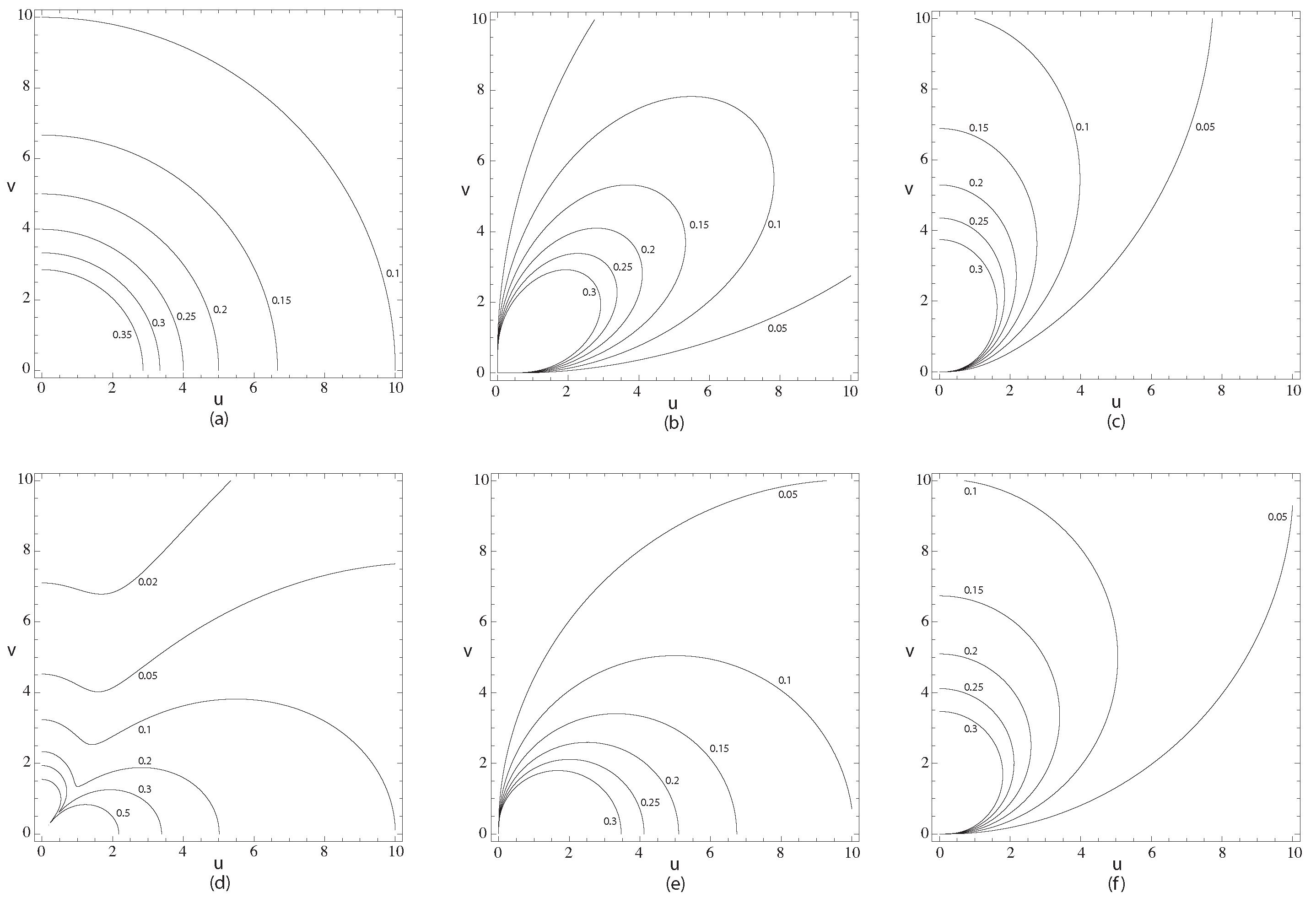
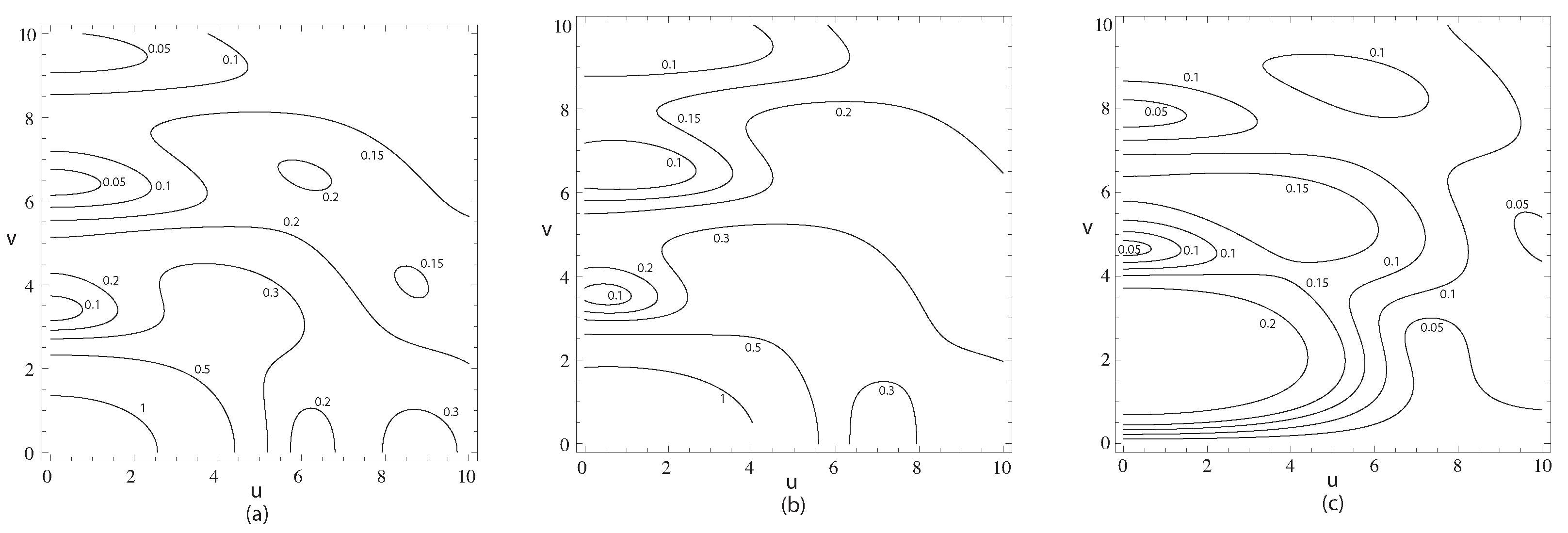
Contours of constant magnitude, in the first quadrant, of the integrals giving the total outgoing electric field are shown in Figure 1. The contours were plotted using Mathematica^TM Version 7.01, Wolfram Research Inc., Champaign, IL, USA. $M_0$ is the total field of a simple source, and so is spherically symmetric. The other integrals correspond to different differentials of the simple source field. All the integrals exhibit singularities at the origin.

The significance of the auxiliary functions for the electric dipole is that the Green tensor can then be written in terms of them, as

$$\mathbf{G}={\displaystyle \frac{k}{2}}\left(\begin{array}{ccc}(M_0+N)-M_{2}cos2\varphi & -M_{2}sin2\varphi & -\mathrm{s}\mathrm{i}\mathrm{g}\mathrm{n}u{M}_{1}cos\varphi \\ -M_{2}sin2\varphi & (M_0+N)+M_{2}cos2\varphi & -\mathrm{s}\mathrm{i}\mathrm{g}\mathrm{n}u{M}_{1}sin\varphi \\ -\mathrm{s}\mathrm{i}\mathrm{g}\mathrm{n}u{M}_{1}cos\varphi & -\mathrm{s}\mathrm{i}\mathrm{g}\mathrm{n}u{M}_{1}sin\varphi & 2(M_0-N)\end{array}\right).$$

(19)

This matrix is symmetric, with trace $2k{M}_0$.

The Green’s (pseudo)vector is [7]

$$\mathbf{g}=k(M_{f}cos\varphi \mathbf{i}+M_{f}sin\varphi \mathbf{j}+\mathrm{s}\mathrm{i}\mathrm{g}\mathrm{n}u{M}_e\mathbf{k}).$$

(20)

The evanescent field is completely contained within the real parts of the auxiliary functions [6,10]. But the real parts also contain a component that is not evanescent, which contributes to the traveling field. On the other hand, the imaginary parts of the auxiliary functions for outgoing dipoles, corresponding to standing waves, are

$$\begin{array}{cc}\hfill \Im \left\{M_0\right\}& ={\displaystyle \frac{sinq}{q}}=i{j}_0\left(q\right),\hfill \\ \hfill \Im \left\{M_1\right\}& ={\displaystyle \frac{i2v\left|u\right|}{q^2}}{j}_2\left(q\right),\hfill \\ \hfill \Im \left\{M_2\right\}& =-{\displaystyle \frac{i{v}^2}{q^2}}{j}_2\left(q\right),\hfill \\ \hfill \Im \left\{N\right\}& =i\left[{\displaystyle \frac{j_1\left(q\right)}{q}}+{\displaystyle \frac{u^2}{q^2}}{j}_2\left(q\right)\right]={\displaystyle \frac{i}{3}}\left[j_0\left(q\right)+\left(1-{\displaystyle \frac{3u^2}{q^2}}\right)j_2\left(q\right)\right],\hfill \\ \hfill \Im \left\{M_e\right\}& ={\displaystyle \frac{i\left|u\right|}{q}}{j}_1\left(q\right),\hfill \\ \hfill \Im \left\{M_f\right\}& ={\displaystyle \frac{iv}{q}}{j}_1\left(q\right).\hfill \end{array}$$

(21)

For a dipole sink, $i{h}_n^{\left(1\right)}\left(q\right)$ is replaced by $i{h}_n^{\left(2\right)}\left(q\right)=y_n\left(q\right)+i{j}_n\left(q\right)$, and the imaginary parts of the auxiliary functions are identical to those of a dipole source in Equation (21).

A full spherical traveling field, in which the wave converges and then diverges from the focus, is given by twice the imaginary part of the source field, the real part canceling, and hence in the equations for the spherical traveling wave, the delta functions in Equation (17) disappear and $i{h}_n^{\left(1\right)}\left(q\right)$ is replaced by $2i{j}_n\left(q\right)$, giving the same as Equations (15) and (16), and twice the values in Equation (21).

6. Evanescent Component

Setälä et al. presented the traveling and evanescent components of the electromagnetic Green tensor in terms of single integrals [8]. Analytical expressions in terms of Lommel functions for the evanescent components of the field for a scalar source and for a scalar dipole source, were presented by Bertilone [4]. Arnoldus and Foley extended this treatment to give, in terms of Lommel functions, the evanescent component of the electric field of an electric dipole, i.e., the evanescent component of the dyadic Green function [6]. In a later paper, Arnoldus considered the magnetic field of an electric dipole, analogous in form to the electric field of a magnetic dipole, and gave solutions as sums of Bessel functions, but not, in this case, in terms of Lommel functions [7]. Here, we give expressions for all the components in terms of Lommel functions. In particular, we present expressions for $M_e^{ev}$ and $M_f^{ev}$, and also $M_1^{ev}$ and $M_2^{ev}$ are written in a more symmetrical way. (The paper for Arnoldus and Foley seems to have an incorrect sign for $2{\zeta }^2{U}_0$ as part of $N^{ev}$ in Equation 71 of Reference [6]). The arguments of the Bessel and Lommel functions are v and $(q-|u|,v)$, respectively, but they have been suppressed for those other than $M_0^{ev}$ for compactness. Then,

$$\begin{array}{cc}\hfill M_0^{ev}& ={\displaystyle \frac{2U_0(q-|u|,v)-J_0\left(v\right)}{\left|q\right|}},\hfill \\ \hfill M_1^{ev}& ={\displaystyle \frac{2}{q^2}}\left[-v{J}_2-{\displaystyle \frac{v\left|u\right|}{q}}\left(1-{\displaystyle \frac{3}{q^2}}\right)(2U_0-J_0)+{\displaystyle \frac{3\left|u\right|}{q^2}}(2v{U}_1+\left|u\right|J_1)\right],\hfill \\ \hfill M_2^{ev}& ={\displaystyle \frac{1}{q^2}}\left[-\left|u\right|J_2+{\displaystyle \frac{v^2}{\left|u\right|q^2}}\left(1-{\displaystyle \frac{3}{q^2}}\right)(2U_0-J_0)-{\displaystyle \frac{3v}{q^2}}(2v{U}_1+\left|u\right|J_1)\right],\hfill \\ \hfill N^{ev}& =-{\displaystyle \frac{8\pi }{3}}\delta \left(\mathbf{q}\right)+{\displaystyle \frac{\left|u\right|}{q^2}}{J}_2+\left(1+{\left|u\right|}^2-{\displaystyle \frac{{3\left|u\right|}^2}{q^2}}\right){\displaystyle \frac{(2U_0-J_0)}{q^3}}+\left(1-{\displaystyle \frac{{3\left|u\right|}^2}{q^2}}\right){\displaystyle \frac{(2v{U}_1+|u\left|J_1\right)}{v{q}^2}},\hfill \\ \hfill M_e^{ev}& ={\displaystyle \frac{4\pi \left|u\right|}{3}}\delta \left(\mathbf{q}\right)+{\displaystyle \frac{1}{q^3}}\left[\left|u\right|(2U_0-J_0)+q\left(2\right|u|U_1-v{J}_1)\right],\hfill \\ \hfill M_f^{ev}& ={\displaystyle \frac{4\pi v}{3}}\delta \left(\mathbf{q}\right)+{\displaystyle \frac{1}{q^3}}\left[v(2U_0-J_0)+q(2v{U}_1+\left|u\right|J_1)\right],\hfill \end{array}$$

(22)

where $U_0,U_1$ are Lommel functions of two variables [11]. Some publications omit the Lommel function for the order 0, but it can be determined from the recurrence relationship $U_0(u,v)=[J_0\left(v\right)-U_2(u,v)]$, so $(2U_0-J_0)=(J_0-2U_2)$ [17]. The factors $(1-3/q^2)$ in Equation (22) are introduced by the spherical Bessel function of the second kind, $y_2\left(q\right)=[q^2(1-3/q^2)cosq-3qsinq]/q^3$.

The integrals in the auxiliary functions can be evaluated using a standard integral given in Reference [39], p.188, no. 2.12.10.3. Arnoldus points out that this contains an error, such that $exp(ia...)$ should be $-iexp(ia...)$ [6]. Arnoldus explains that if $M_0^{ev},M_2^{ev}$ and $M_f^{ev}$ (integrals of $J_0,J_2,J_1$, respectively) are known, then $M_1^{ev},N^{ev}$ and $M_e^{ev}$ can be calculated from them [7]. Setälä et al., on the other hand, express the components in terms of $M_0^{ev},M_e^{ev}$ and $N^{ev}$, which are all integrals of $J_0$ [8]. Various differential relationships also exist between the functions.

For our form of the evanescent auxiliary functions, giving the evanescent parts of a dipole sink for $u<0$ and a dipole source for $u>0$, respectively, the arguments of the Bessel and Lommel functions are taken as v and $(w-u,v)$, respectively. Then,

$$\begin{array}{cc}\hfill M_0^{ev}& ={\displaystyle \frac{2U_0(w-u,v)-J_0\left(v\right)}{w}},\hfill \\ \hfill M_1^{ev}& ={\displaystyle \frac{2}{w^2}}\left[-v{J}_2-{\displaystyle \frac{vu}{w}}\left(1-{\displaystyle \frac{3}{w^2}}\right)(2U_0-J_0)+{\displaystyle \frac{3u}{w^2}}(2v{U}_1+u{J}_1)\right],\hfill \\ \hfill M_2^{ev}& ={\displaystyle \frac{1}{w^2}}\left[-u{J}_2+{\displaystyle \frac{v^2}{u{w}^2}}\left(1-{\displaystyle \frac{3}{w^2}}\right)(2U_0-J_0)-{\displaystyle \frac{3v}{w^2}}(2v{U}_1+u{J}_1)\right],\hfill \\ \hfill N^{ev}& ={\displaystyle \frac{u}{w^2}}{J}_2+\left(1+u^2-{\displaystyle \frac{3u^2}{w^2}}\right){\displaystyle \frac{(2U_0-J_0)}{w^3}}+\left(1-{\displaystyle \frac{3u^2}{w^2}}\right){\displaystyle \frac{(2v{U}_1+u{J}_1)}{v{w}^2}},\hfill \\ \hfill M_e^{ev}& ={\displaystyle \frac{1}{w^3}}\left[u(2U_0-J_0)+w(2u{U}_1-v{J}_1)\right],\hfill \\ \hfill M_f^{ev}& ={\displaystyle \frac{1}{w^3}}\left[v(2U_0-J_0)+w(2v{U}_1+u{J}_1)\right],\hfill \end{array}$$

(23)

where $w=\pm q$ and $(w-u)=\pm (q-|u\left|\right)$ are odd functions of u. $M_1^{ev}$ and $M_e^{ev}$ are real and even functions of u; $M_0^{ev}$, $M_2^{ev}$, $N^{ev}$, and $M_f^{ev}$ are real and odd functions of u. The self-field now cancels, as there is no net source. The auxiliary functions are purely real and satisfy the relationships

$$\begin{array}{cc}\hfill v{M}_1^{ev}+2u{M}_2^{ev}=& -2J_2\left(v\right),\hfill \\ \hfill v{M}_e^{ev}-u{M}_f^{ev}=& -J_1\left(v\right),\hfill \\ \hfill N^{ev}=& \frac{1}{3}\left(M_0^{ev}-{\displaystyle \frac{u}{v}}{M}_1^{ev}-M_2^{ev}\right),\hfill \\ \hfill M_f^{ev}=& \frac{1}{2}v(M_0^{ev}-M_2^{ev}-N^{ev}),\hfill \end{array}$$

(24)

which are the same as given by Arnoldus, but with u instead of $\left|u\right|$ [6,7]. If we compare these equations with those in Equation (18), we see that the Bessel functions $J_1,J_2$ in the evanescent parts must cancel with similar functions with opposite signs in the traveling part. These contributions result from a polarized Bessel beam generated by scattering from the edge of the hemispherical aperture [23].

The expressions for the evanescent parameters can be written in a compact form by introducing the functions

$$\begin{array}{cc}\hfill {\mathrm{\Lambda }}_0(u,v)=& {\displaystyle \frac{2U_0(w-u,v)-J_0\left(v\right)}{w}},\hfill \\ \hfill {\mathrm{\Lambda }}_1(u,v)=& {\displaystyle \frac{2v{U}_1(w-u,v)+u{J}_1\left(v\right)}{w^2}},\hfill \end{array}$$

(25)

where ${\mathrm{\Lambda }}_1$ follows naturally from the equation for $M_f^{ev}$ in Equation (23). ${\mathrm{\Lambda }}_0(u,v)$ and ${\mathrm{\Lambda }}_1(u,v)$ are both odd functions of u. (The corresponding forms of these functions with w replaced by $\left|q\right|$ can also be used for the auxiliary functions of Arnoldus).

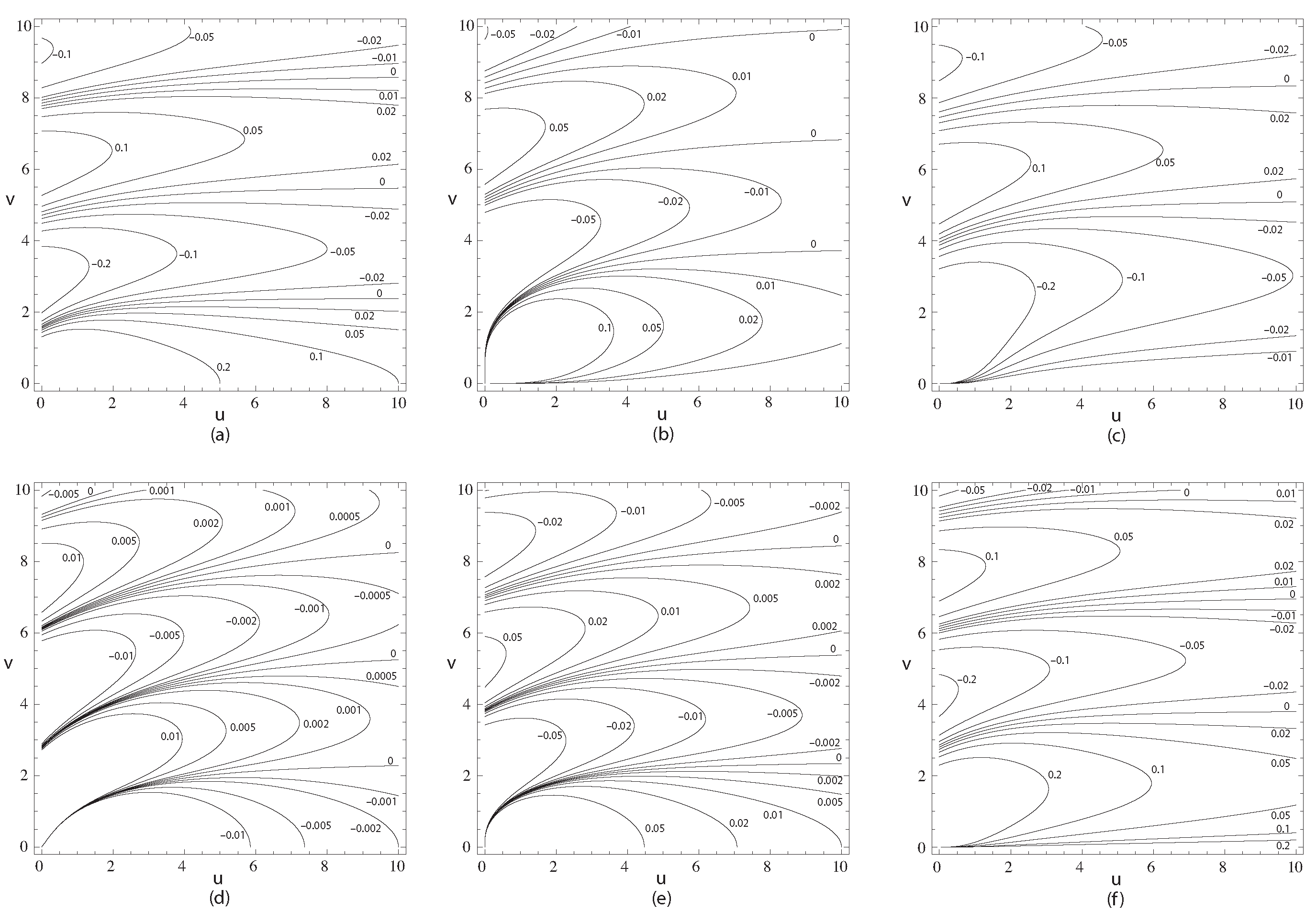
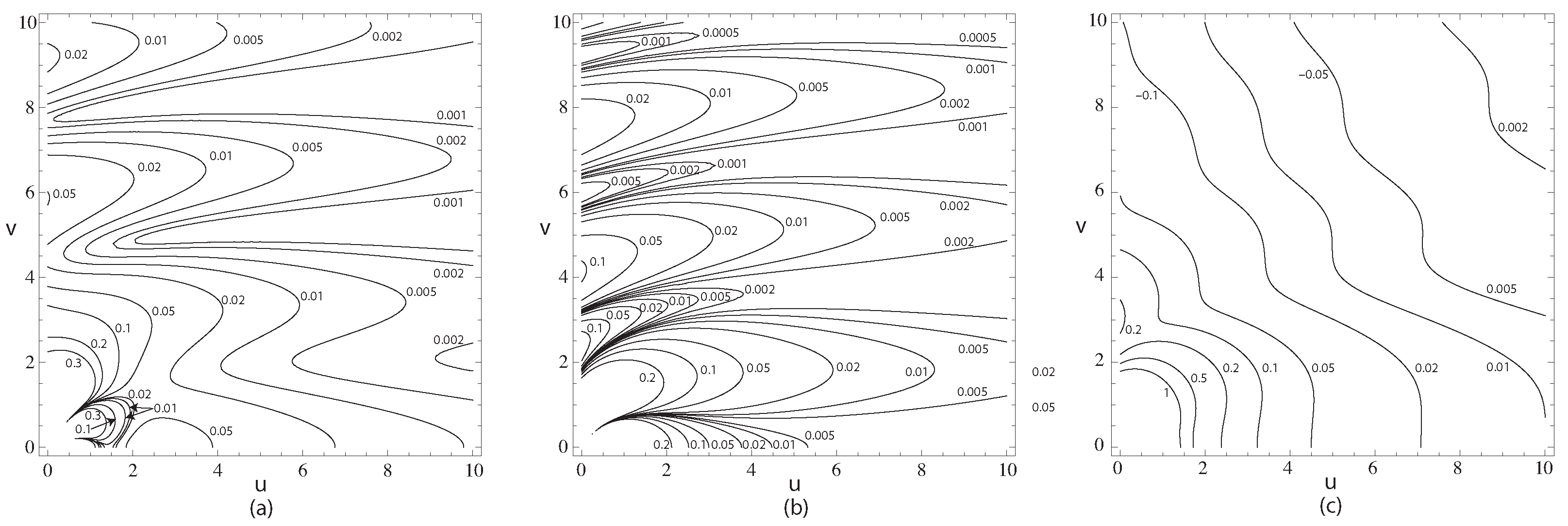
We then have for our forms of the auxiliary functions,

$$\begin{array}{cc}\hfill M_0^{ev}& ={\mathrm{\Lambda }}_0,\hfill \\ \hfill M_1^{ev}& ={\displaystyle \frac{2}{w^2}}\left[-v{J}_2\left(v\right)-uv\left(1-{\displaystyle \frac{3}{w^2}}\right){\mathrm{\Lambda }}_0+3u{\mathrm{\Lambda }}_1\right],\hfill \\ \hfill M_2^{ev}& ={\displaystyle \frac{1}{w^2}}\left[-u{J}_2\left(v\right)+v^2\left(1-{\displaystyle \frac{3}{w^2}}\right){\mathrm{\Lambda }}_0-3v{\mathrm{\Lambda }}_1\right],\hfill \\ \hfill N^{ev}& ={\displaystyle \frac{u\left(J_2\left(v\right)+u{\mathrm{\Lambda }}_0\right)}{w^2}}+\left(1-{\displaystyle \frac{3u^2}{w^2}}\right){\displaystyle \frac{(v{\mathrm{\Lambda }}_0+w^2{\mathrm{\Lambda }}_1)}{v{w}^2}}\hfill \\ \hfill M_e^{ev}& ={\displaystyle \frac{u{\mathrm{\Lambda }}_0}{w^2}}+{\displaystyle \frac{u}{v}}{\mathrm{\Lambda }}_1-{\displaystyle \frac{J_1\left(v\right)}{v}},\hfill \\ \hfill M_f^{ev}& ={\displaystyle \frac{v{\mathrm{\Lambda }}_0}{w^2}}+{\mathrm{\Lambda }}_1.\hfill \end{array}$$

(26)

Written in this way, it is easy to see that they satisfy the relationships in Equation (24). For positive u, both forms of the auxiliary functions are identical and real, and contours of constant value are shown in Figure 2.

In the plane of the dipole, $u=0$, $U_0(v,v)=[J_0\left(v\right)+cosv]/2$, $U_1(v,v)=(sinv)/2$, ${\mathrm{\Lambda }}_0(v,v)=(cosv)/v=-y_0\left(v\right)$, ${\mathrm{\Lambda }}_1(v,v)=(sinv)/v=j_0\left(v\right)$, and we obtain

$$\begin{array}{cc}\hfill M_0^{ev}=& {\displaystyle \frac{cosv}{v}}=-y_0\left(v\right),\hfill \\ \hfill M_1^{ev}=& -{\displaystyle \frac{2J_2\left(v\right)}{v}}=-\frac{1}{2}\left[J_1\left(v\right)+J_3\left(v\right)\right],\hfill \\ \hfill M_2^{ev}=& y_2\left(v\right),\hfill \\ \hfill N^{ev}=& -{\displaystyle \frac{y_1\left(v\right)}{v}}=-\frac{1}{3}\left[y_0\left(v\right)+y_2\left(v\right)\right],\hfill \\ \hfill M_e^{ev}=& -{\displaystyle \frac{J_1\left(v\right)}{v}}=-\frac{1}{2}\left[J_0\left(v\right)+J_2\left(v\right)\right],\hfill \\ \hfill M_f^{ev}=& -y_1\left(v\right),\hfill \end{array}$$

(27)

in agreement with References [6,7,8].

7. Traveling Component

Once we have the evanescent components, the traveling components for non-negative u can calculated from $M_n^{tr}=M_n-M_n^{ev}$:

$$\begin{array}{cc}\hfill M_0^{tr}& =i{h}_0^{\left(1\right)}\left(w\right)-{\mathrm{\Lambda }}_0,\hfill \\ \hfill M_1^{tr}& ={\displaystyle \frac{i2vu}{w^2}}{h}_2^{\left(1\right)}\left(w\right)-{\displaystyle \frac{2}{w^2}}\left[-v{J}_2\left(v\right)-vu\left(1-{\displaystyle \frac{3}{w^2}}\right){\mathrm{\Lambda }}_0+3u{\mathrm{\Lambda }}_1\right],\hfill \\ \hfill M_2^{tr}& =-{\displaystyle \frac{i{v}^2}{w^2}}{h}_2^{\left(1\right)}\left(w\right)-{\displaystyle \frac{1}{w^2}}\left[-u{J}_2\left(v\right)+v^2\left(1-{\displaystyle \frac{3}{w^2}}\right){\mathrm{\Lambda }}_0-3v{\mathrm{\Lambda }}_1\right],\hfill \\ \hfill N^{tr}& ={\displaystyle \frac{i}{3}}{h}_0^{\left(1\right)}\left(w\right)+{\displaystyle \frac{i}{3}}\left(1-{\displaystyle \frac{3u^2}{w^2}}\right)h_2^{\left(1\right)}\left(w\right)-{\displaystyle \frac{u\left(J_2\left(v\right)+u{\mathrm{\Lambda }}_0\right)}{w^2}}-\left(1-{\displaystyle \frac{3u^2}{w^2}}\right){\displaystyle \frac{\left(v{\mathrm{\Lambda }}_0+w^2{\mathrm{\Lambda }}_1\right)}{v{w}^2}}\hfill \\ \hfill M_e^{tr}& =iu{\displaystyle \frac{h_1^{\left(1\right)}\left(w\right)}{w}}-{\displaystyle \frac{u{\mathrm{\Lambda }}_0}{w^2}}-{\displaystyle \frac{u}{v}}{\mathrm{\Lambda }}_1+{\displaystyle \frac{J_1\left(v\right)}{v}},\hfill \\ \hfill M_f^{tr}& =iv{\displaystyle \frac{h_1^{\left(1\right)}\left(w\right)}{w}}-{\displaystyle \frac{v{\mathrm{\Lambda }}_0}{w^2}}-{\mathrm{\Lambda }}_1.\hfill \end{array}$$

(28)

The imaginary parts of the traveling components are equal to the imaginary parts of the total auxiliary functions, as the evanescent components are purely real.

Contours of constant magnitude of the traveling components are shown in Figure 3. $M_0^{tr}$ is the same as the amplitude for a simple scalar source and is equal to unity at the origin [40]. Also, $N^{tr}=1/3$ and $M_e^{tr}=1/2$ at the origin. All the other auxiliary functions are zero at the origin.

8. Field in the Focal Region for Hemispherical Focusing

For hemispherical focusing in the Debye approximation, there is no evanescent field. From the auxiliary functions, we can obtain the integrals $I_n^{\left(p\right)},I_n^{\left(mg\right)}$. For example, $I_0^{\left(p\right)}=-i(M_0^{tr}+N^{tr})$. We have

$$\begin{array}{cc}\hfill I_0^{\left(p\right)}& =-i{e}^{iv}(1-iv+v^2)+{\displaystyle \frac{i[u{J}_0\left(v\right)+(w^2+u^2){\mathrm{\Lambda }}_0]}{w^2}}+i\left(1-{\displaystyle \frac{3u^2}{w^2}}\right){\displaystyle \frac{\left(v{\mathrm{\Lambda }}_0+w^2{\mathrm{\Lambda }}_1\right)}{v{w}^2}},\hfill \\ \hfill I_1^{\left(p\right)}& ={\displaystyle \frac{ivu}{w^2}}{h}_2^{\left(1\right)}\left(w\right)-{\displaystyle \frac{1}{w^2}}\left[-v{J}_2\left(v\right)-vu\left(1-{\displaystyle \frac{3}{w^2}}\right){\mathrm{\Lambda }}_0+3u{\mathrm{\Lambda }}_1\right],\hfill \\ \hfill I_2^{\left(p\right)}& ={\displaystyle \frac{v^2}{w^2}}{h}_2^{\left(1\right)}\left(w\right)-{\displaystyle \frac{i}{w^2}}\left[-u{J}_2\left(v\right)+v^2\left(1-{\displaystyle \frac{3}{w^2}}\right){\mathrm{\Lambda }}_0-3v{\mathrm{\Lambda }}_1\right],\hfill \\ \hfill I_0^{\left(mg\right)}& =2iu{\displaystyle \frac{h_1^{\left(1\right)}\left(w\right)}{w}}-{\displaystyle \frac{2u{\mathrm{\Lambda }}_0}{w^2}}-{\displaystyle \frac{2u}{v}}{\mathrm{\Lambda }}_1+{\displaystyle \frac{2J_1\left(v\right)}{v}},\hfill \\ \hfill I_1^{\left(mg\right)}& =v{\displaystyle \frac{h_1^{\left(1\right)}\left(w\right)}{w}}+{\displaystyle \frac{iv{\mathrm{\Lambda }}_0}{w^2}}+i{\mathrm{\Lambda }}_1.\hfill \end{array}$$

(29)

Contours of constant magnitude of $(M_0+N)$ for the total, and evanescent and traveling components, are shown in Figure 4, Figure 5 and Figure 6, parts (a). At the origin, $(M_0^{tr}+N^{tr})=4/3$.

The auxiliary functions for the traveling component are related to the parameters $I_0^H,I_1^H,I_2^H,L_1^H,L_2^H,L_3^H$ of Setälä et al. by the following relationships: $M_0^{tr}=i{I}_0^H$, $M_e^{tr}=I_1^H$, $N^{tr}=i{I}_2^H$, $M_f^{tr}=i{L}_1^H$, $M_1^{tr}=2L_3^H$, $(M_0^{tr}-N^{tr})=i{L}_2^H$, $M_2^{tr}=-i(2L_1^H/v-L_2)$ [8].

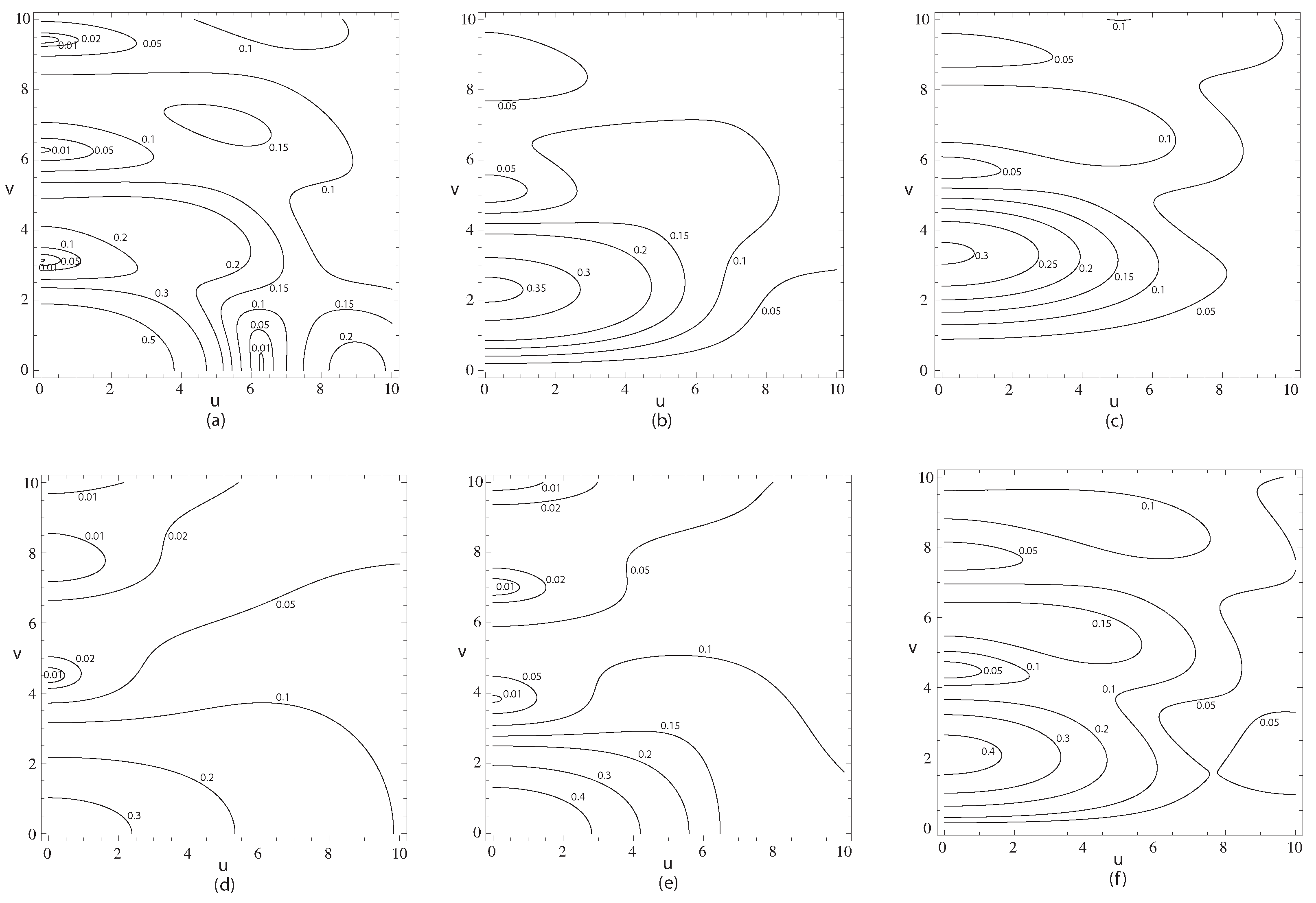
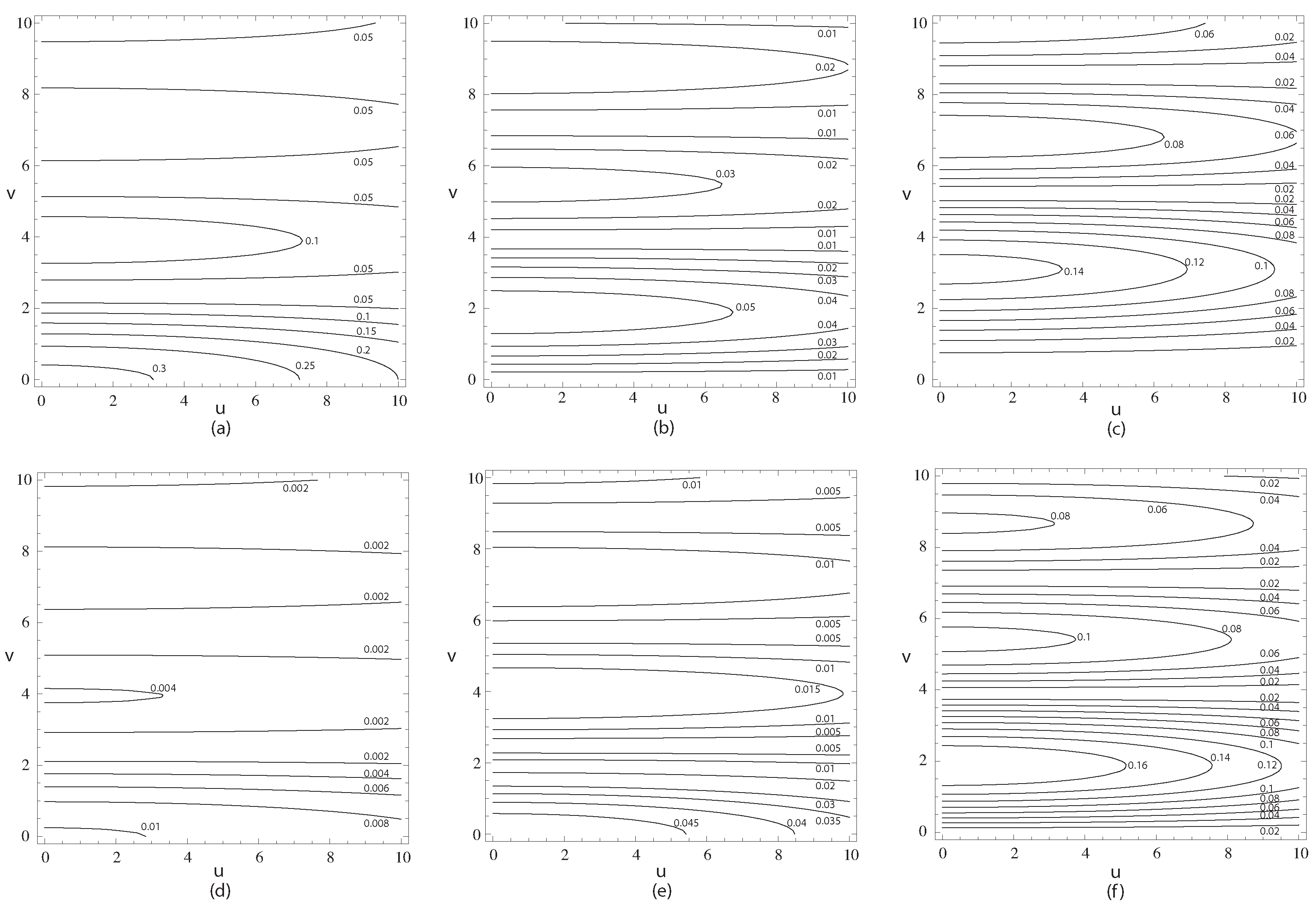
9. Mixed Dipole Case

The integrals $I_n$ for the mixed dipole (MxD) case can then be obtained from $(I_n^{\left(p\right)}+I_n^{\left(mg\right)})$. In Figure 4, Figure 5 and Figure 6, we show contours of constant magnitude of $(M_0+N+2i{M}_e)$ and $(M_1/2-i{M}_f)$, in parts (b) and (c), respectively. For Figure 6, $(M_0^{tr}+N^{tr}+2i{M}_e^{tr})=i\left(I_0^{\left(p\right)}+I_0^{\left(mg\right)}\right)$ and $(M_1^{tr}/2-i{M}_f^{tr})=\left(I_1^{\left(p\right)}+I_1^{\left(mg\right)}\right)$. At the origin, $(M_0^{tr}+N^{tr}+2i{M}_e^{tr})=7i/3$.

In the plane of the dipole, $u=0$, we have

$$\begin{array}{cc}\hfill M_0^{tr}=& i{\displaystyle \frac{sinv}{v}}=i{j}_0\left(v\right),\hfill \\ \hfill M_1^{tr}=& {\displaystyle \frac{2J_2\left(v\right)}{v}}=\frac{1}{2}\left[J_1\left(v\right)+J_3\left(v\right)\right],\hfill \\ \hfill M_2^{tr}=& -i{j}_2\left(v\right),\hfill \\ \hfill N^{tr}=& i{\displaystyle \frac{j_1\left(v\right)}{v}}=-{\displaystyle \frac{i}{3}}\left[j_0\left(v\right)+j_2\left(v\right)\right],\hfill \\ \hfill M_e^{tr}=& {\displaystyle \frac{J_1\left(v\right)}{v}}=\frac{1}{2}\left[J_0\left(v\right)+J_2\left(v\right)\right],\hfill \\ \hfill M_f^{tr}=& i{j}_1\left(v\right),\hfill \end{array}$$

(30)

agreeing with Arnoldus [7]. Then,

$$\begin{array}{cc}\hfill I_0^{\left(p\right)}& =-i(M_0^{tr}+N^{tr})=j_0\left(v\right)+{\displaystyle \frac{j_1\left(v\right)}{v}}=\frac{1}{3}[4j_0\left(v\right)+j_2\left(v\right)],\hfill \\ \hfill I_1^{\left(p\right)}& ={\displaystyle \frac{J_2\left(v\right)}{v}},\hfill \\ \hfill I_2^{\left(p\right)}& =j_2\left(v\right),\hfill \\ \hfill I_0^{\left(mg\right)}& ={\displaystyle \frac{2J_1\left(v\right)}{v}}=J_0\left(v\right)+J_2\left(v\right),\hfill \\ \hfill I_1^{\left(mg\right)}& =j_1\left(v\right),\hfill \end{array}$$

(31)

agreeing with results published previously for the focal plane with hemispherical focusing [1,33]. Note, however, that in the present paper, we have taken the traveling field at the focus to be purely imaginary so that the evanescent component is purely real, in accordance with the treatments of Richards and Wolf, and with Arnoldus [7,20].

The fields of transverse electric or magnetic dipoles are not cylindrically symmetric about the axis, but cylindrically symmetric forms, corresponding to rotating dipoles or focused circular polarized light, can be formed. For simplicity, we define electric energy density $W_E$ as the squared magnitude of the electric field. Contours of constant electric energy density in an azimuthal plane for rotating ED, rotating MgD, and rotating MxD polarizations, of the total, and evanescent and traveling components, are shown in Figure 7, Figure 8, and Figure 9, respectively. The MxD case in Figure 9c corresponds to hemispherical focusing of a circularly polarized mixed dipole wave.

The electric energy densities at the origin for the traveling components are 16/9 for electric dipole polarization, 1 for magnetic dipole polarization, and 49/9 for mixed dipole polarization. The FWHM (full width at half maximum) in the focal plane is $v=3.10, 5.02$ and $3.64$, for ED, MgD, and MxD, respectively [1].

10. The Field in the Focal Region for a Lens of Lower Numerical Aperture

While the analytical results described here are calculated for a hemispherical focusing system, they give approximate results for practical systems such as lenses of high numerical aperture but for less than a hemisphere, like a dry objective of 0.95 NA or an oil immersion lens of 1.4 NA [1]. For the dipole cases considered, the field is still appreciable at the edge of the hemispherical aperture (except for the $M_1$, $M_e$, and N components), which, therefore, by the principle of stationary phase, can contribute appreciably to the focused field.

For close to hemispherical focusing, a better approximation to the focused field can be obtained by subtracting from the unnormalized hemispherical field for an annular aperture [1]. For a narrow annulus, the field can be approximated [41,42]. In the limit, the field of the annulus is given by a vectorial Bessel beam, for which $M_0^{ann}=J_0\left(v\right)$, $M_2^{ann}=-J_2\left(v\right)$, $M_f^{ann}=J_1\left(v\right)$, and $M_1^{ann}=N^{ann}=M_e^{ann}=0$. Refs. [1,23,43,44,45]. These correspond to $I_0^{\left(p\right)}=-i{J}_0\left(v\right)$, $I_2^{\left(p\right)}=-i{J}_2\left(p\right)$, $I_1^{\left(mg\right)}=-i{J}_1\left(v\right)$, and $I_1^{\left(p\right)}=I_0^{\left(mg\right)}=I_2^{\left(mg\right)}=0$.

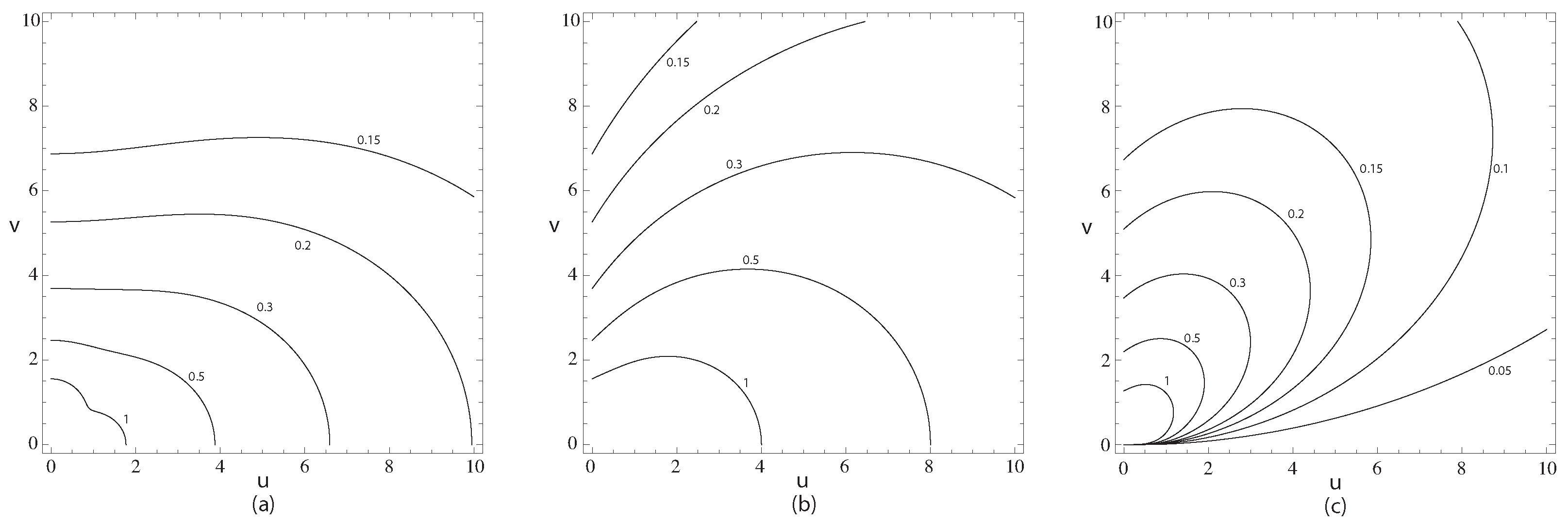
Contours of constant magnitude of the auxiliary functions for an annulus of outer NA of 1 and inner NA of 0.95 are shown in Figure 10. The plots are stretched out in the u direction, characteristic of an approximation to a Bessel beam. The values of $M_1^{ann}$, $M_e^{ann}$, and, especially, $N^{ann}$ are weak. The value of $M_0^{ann}$ at the focus is 0.312, compared with unity for $M_0^{tr}$, and $N^{ann}=0.010$, compared with $N^{tr}=1/3$.

For 0.99 NA, the value of $M_0^{ann}$ at the focus is 0.141 and $N^{ann}=9.36\times {10}^{-4}$. In this case, the Bessel beam approximation is good for $u<10$. The approximation as a Bessel beam is the same as a right Riemann sum (rectangle rule), with just a single interval. For somewhat lower NAs, the effect of the annulus can be better approximated by interference between two vectorial Bessel beams, scattered from the outer and inner edges of the annular region, and equivalent to numerical integration using the trapezoidal rule with a single interval.

11. Discussion

Analytic forms, in terms of Lommel functions of two variables, for the evanescent and traveling parts of the electromagnetic Green tensor have been presented. The field in the focal region, including defocus, of hemispherically focused electric dipole, magnetic dipole, and mixed dipole waves, has been expressed analytically in closed form. Extension to the case of high numerical apertures less than a complete hemisphere was considered.