Combining Kronecker-Basis-Representation Tensor Decomposition and Total Variational Constraint for Spectral Computed Tomography Reconstruction

Abstract

Energy spectrum computed tomography (CT) technology based on photon-counting detectors has been widely used in many applications such as lesion detection, material decomposition, and so on. But severe noise in the reconstructed images affects the accuracy of these applications. The method based on tensor decomposition can effectively remove noise by exploring the correlation of energy channels, but it is difficult for traditional tensor decomposition methods to describe the problem of tensor sparsity and low-rank properties of all expansion modules simultaneously. To address this issue, an algorithm for spectral CT reconstruction based on photon-counting detectors is proposed, which combines Kronecker-Basis-Representation (KBR) tensor decomposition and total variational (TV) regularization (namely KBR-TV). The proposed algorithm uses KBR tensor decomposition to unify the sparse measurements of traditional tensor spaces, and constructs a third-order tensor cube through non-local image similarity matching. At the same time, the TV regularization term is introduced into the independent energy spectrum image domain to enhance the sparsity constraint of single-channel images, effectively reduce artifacts, and improve the accuracy of image reconstruction. The proposed objective minimization model has been tackled using the split-Bregman algorithm. To evaluate the algorithm’s performance, both numerical simulations and realistic preclinical mouse studies were conducted. The ultimate findings indicate that the KBR-TV method offers superior enhancement in the quality of spectral CT images in comparison to several existing methods.

1. Introduction

X-ray computed tomography (CT) represents a non-invasive imaging modality that offers insights into the internal architecture of organs, finding extensive utility across biomedical imaging, safety inspection, material analysis, and so on [1,2]. Despite its broad applications, conventional CT technology faces certain limitations, including the absence of energy-resolved information and the presence of pronounced beam hardening artifacts in the acquired images [3,4]. Furthermore, acquiring multiple energy projections necessitates multiple scans, thereby elevating the associated radiation risk [5,6]. To address these challenges, spectral CT employing photon-counting detectors has garnered considerable attention due to its ability to furnish spectral data [7]. Photon-counting detectors can distinguish the energy of X-ray photons according to the predetermined energy threshold, effectively identify and record the photons in the corresponding energy channels, and obtain the projection data of multiple channels at the same time. However, single-channel projections are often plagued by significant quantum noise stemming from the scarcity of photons in the respective energy bins, leading to a substantial decrement in image quality [8]. As a result, improving the quality of spectral CT images has become a key area of focus in research activities.

To enhance the quality of spectral CT images derived from noisy projections, a multitude of algorithms have been proposed. Initially, conventional CT reconstruction techniques were adapted for this purpose. Xu et al. subsequently proposed reconstruction models based on TV, dictionary learning, and dictionary learning combined with low-rank constraints, applying these constraints to CT images across all energy channels, thereby augmenting the spectral CT imaging quality [9,10,11]. Zhao et al. introduced a novel iterative reconstruction (IR) algorithm based on dual-dictionary learning (DDL) and tight frame (TFIR) for breast spectral CT imaging, which demonstrated superior reconstruction outcomes with sparse projection data [12,13]. In 2016, Zeng et al. presented a penalized weighted least-squares (PWLS) scheme by incorporating the new concept of structure tensor total variation (STV) regularization (namely PWLS-STV), yielding spectral CT images of superior quality [14]. Wang et al. employed a refined locally linear transform to convert the structural similarity among two-dimensional (2D) spectral CT images into a spectral-dimension gradient sparsity, which improved reconstruction quality and decomposition accuracy [15]. However, a common limitation of these approaches is that CT images from different energy channels were processed independently during the reconstruction phase, focusing solely on intra-channel correlations.

To overcome the limitations of the above algorithm and explore the correlations inherent in images across different energy channels, an increasing number of algorithms are adopting tensor models for multispectral CT image representation. These algorithms utilize prior information embedded within tensors (e.g., sparsity, low-rankness) to enhance the quality of spectral CT images. Gao et al. introduced a reconstruction model known as PRISM, which leveraged prior rank, intensity, and sparsity for image reconstruction [16]. Then, Li et al. proposed a new tensor PRISM model that consistently incorporated a priori knowledge of low-rank property, intensity and sparsity with higher-dimensional tensor techniques, effectively exploiting similarities across the energy dimension [17]. Rigie et al. employed total nuclear variation (TNV) as a regularizer for the reconstruction of multi-channel spectral CT images, leveraging its ability to promote shared edge locations and a common gradient direction across image channels, which effectively preserved image edges and yielded better results [18]. He et al. combined the nuclear norm with bilateral weighted relative total variation (BRTV) for spectral CT reconstruction, which effectively captured inter-channel correlations and extracted intra-channel structures, thereby improving image quality [19]. In recent years, tensor dictionary learning (TDL) has emerged as a promising approach for spectral computed tomography (CT) image reconstruction, demonstrating significant capabilities in noise suppression and detail preservation. A notable advancement was made by Zhang et al. in 2017, who developed a TDL-based reconstruction framework that integrates tensor operations with sparse dictionary representations, achieving effective noise reduction and detail recovery [20]. Later, Wu et al. enhanced this framework by incorporating the L₀ norm of the image gradient, which proved particularly effective in maintaining edge sharpness and structural details when processing low-dose and sparse-view projection data [21]. Further improvements were introduced by Li et al., who extended the sparsity-constrained TDL algorithm by incorporating both image gradient L₀ norm constraints and full-spectrum image correlations within the TDL framework, leading to enhanced reconstruction performance [22]. While these TDL-based methods have demonstrated considerable success, it is important to note that reconstruction quality remains critically dependent on the quality and representativeness of the training tensor dictionary datasets.

Subsequently, tensor decomposition has emerged as a potent technique for representing and analyzing images, which can effectively mitigate noise and artifacts [23,24]. It has been widely applied in diverse fields, including signal processing, video data analysis, and hyperspectral image denoising [25,26,27]. Because of the analogies between spectral CT images and multi-dimensional datasets, tensor decomposition techniques can be adapted for the purpose of reconstructing spectral CT images. In this context, Zhang et al. proposed an innovative approach for spectral CT image denoising by integrating tensor decomposition with non-local means (TDNLM), demonstrating superior capabilities in recovering intricate details within spectral CT images [28]. Hu et al. proposed an algorithm termed spectral-image similarity-based tensor with enhanced-sparsity reconstruction (SISTER), which significantly enhanced edge preservation, detailed feature restoration, and noise reduction in the reconstructed image [29].

Wu et al. developed an L₀-norm constrained weighted bilateral image gradient framework integrated with tensor decomposition, achieving enhanced suppression of image artifacts and noise contamination in spectral CT datasets [30]. Wang et al. proposed an image-spectral decomposition with extended learning assisted by sparsity (IDEAS) method, which employed a non-local low-rank Tucker decomposition to fully exploit intrinsic priors to improve multi-energy CT image quality [31]. Chen et al. developed a spectral CT reconstruction algorithm based on fourth-order non-local tensor decomposition, which synergistically combined adaptive weighting kernels with total variation constraints to regulate tensor units, demonstrating superior noise and artifact suppression capabilities [32]. Li et al. established a hybrid reconstruction framework incorporating tensor decomposition with total generalized variation (TGV) regularization, significantly improving sparse-view spectral CT image quality through complementary spatial–spectral constraints [33]. In contrast to algorithms based on tensor dictionary learning, tensor decomposition eliminates the need for pre-trained dictionaries, thus avoiding instabilities caused by the dictionary’s reliance on training data quality in dictionary-based approaches. However, the aforementioned spectral CT reconstruction algorithms based on tensor decomposition primarily employ the Tucker decomposition and CP decomposition as the two main tensor decomposition techniques. From a theoretical perspective, CP decomposition does not fully exploit the low-rank property of subspaces unfolded along the tensor modes, whereas the Tucker decomposition has difficulties exploiting the sparsity of the core tensor [34]. To simultaneously characterize both the sparsity of the tensor and the low-rank nature of all unfolded modes, the Kronecker-Basis-Representation (KBR) tensor decomposition method has been proposed and applied to multispectral image denoising and completion problems, achieving promising results [35,36]. In the field of CT imaging, considering the dynamic nature of perfusion CT images, which continually change over time, KBR has been utilized in low-dose dynamic perfusion CT imaging [37].

In this paper, considering the similarities between X-ray energy spectrum CT images and perfusion CT images, the KBR tensor decomposition algorithm is introduced into energy spectrum CT image reconstruction. At the same time, to enhance the sparsity constraint in the single-channel image domain, this paper integrates a simple and effective TV algorithm into the reconstruction framework, and proposes an energy spectrum CT image reconstruction algorithm combining KBR tensor decomposition and total variational TV, which is called KBR-TV. The proposed KBR-TV method uses non-local image similarity matching to construct a third-order tensor cube. Furthermore, KBR tensor decomposition is used to explore the correlation between energy spectrum channels, replacing the traditional Tucker decomposition and CP decomposition and unifying the sparse metric of the traditional tensor space. Moreover, the TV regularization term is introduced into the independent energy spectrum image domain to enhance the sparsity constraint of the single-channel image, effectively reducing the artifacts caused by the aggregation of image blocks in the tensor decomposition. The introduction of TV not only avoids significantly increasing the running time but also improves the accuracy of reconstruction. The final experimental findings indicate that the KBR-TV algorithm results in reconstructed images of superior quality, with reduced noise artifacts and enhanced detail retention.

The primary contributions of this paper are threefold. Firstly, the proposed algorithm uses KBR tensor decomposition to replace the traditional Tucker decomposition and CP decomposition and unifies the sparse metric of the traditional tensor space. Secondly, in order to balance the low-rank property of the space–energy spectrum domain and the sparsity of the spatial domain, the TV prior is introduced into the reconstruction framework, which effectively reduces the artifacts in the single-channel image domain without excessively increasing the algorithm running time. Lastly, the proposed reconstruction model is tackled using an effective split-Bregman algorithm.

The structure of the subsequent sections of this paper is outlined as follows. Section 2 offers a concise overview of the pertinent mathematical foundations. Section 3 presents the mathematical model underlying the KBR-TV algorithm along with its solution methodology. In Section 4, we conduct comprehensive experiments using both numerically simulated data and preclinical datasets. Lastly, Section 5 summarizes our conclusions and discussion.

2. Fundamental Theory Methods

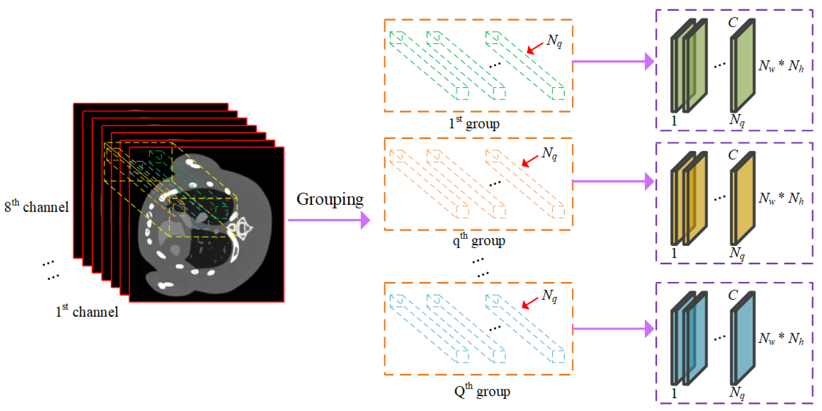
2.1. KBR Tensor Decomposition

The principle of the KBR tensor decomposition involves approximating the original high-order tensor by representing it as a product of a series of lower-order tensors. Specifically, KBR employs the Kronecker product (also known as the direct product) to combine multiple lower-order tensors into a high-order tensor. Subsequently, an appropriate basis representation is selected to decompose the high-order tensor into a linear combination of these lower-order tensors. KBR decomposition integrates the respective advantages of both Canonical Polyadic (CP) decomposition and the Tucker decomposition while overcoming their limitations, which can be expressed as follows:

$$\Im \left(\mathcal{X}\right)={‖\mathcal{M}‖}_0+\delta {\displaystyle \prod _{r=1}^{R}rank\left({\mathit{X}}_{\left(r\right)}\right)}$$

(1)

where $\mathcal{X}\in {ℝ}^{N_1\times N_2\times C}$ is the third-order spectral CT image tensor to be reconstructed; N₁ and N₂ represent the width and height of the reconstructed image, respectively. $\mathcal{M}$ is the core tensor, which is obtained by the Higher-Order Singular Value Decomposition (HOSVD) tensor $\mathcal{X}$. X_(r) is the subspace expanded along the tensor modulus. δ is the parameter greater than 0, which is used to balance the two terms in the equation. In Equation (1), the first term is used to limit the number of Kronecker bases representing the tensor $\mathcal{X}$, which is consistent with the definition of CP tensor decomposition. The second term describes the low-rank properties of the expansion module of the tensor in all directions. Equation (1) reveals the advantage of KBR decomposition, compared to CP decomposition and the Tucker decomposition, which can simultaneously describe the core tensor $\mathcal{M}$ and the tensor in all expansion modules (r = 1, …, R) and unify the sparse metric of traditional tensor spaces.

In order to improve computational efficiency in practical applications, the L₀ norm and low-rank constraint in the KBR method are relaxed and expressed in logarithmic form. Equation (1) can be further rewritten as follows:

$$\Im \left(\mathcal{X}\right)=P\left(\mathcal{M}\right)+\delta {\displaystyle \prod _{r=1}^R{P}^{*}\left({\mathit{X}}_{\left(r\right)}\right)}$$

(2)

Each sub-formula in Equation (2) can be expressed as follows:

$$P\left(\mathcal{M}\right)={\displaystyle \sum _{i_1,\dots i_N}\left(\log \left(\left|m_{i_1,\dots i_N}+\epsilon \right|\right)-\log \left(\epsilon \right)\right)}/\left(-\log \left(\epsilon \right)\right)$$

(3)

$$P^{*}\left({\mathit{X}}_{\left(r\right)}\right)={\displaystyle \sum _n\left(\log \left({\sigma }_n\left({\mathit{X}}_{\left(r\right)}\right)+\epsilon \right)-\log \left(\epsilon \right)\right)/\left(-\log \left(\epsilon \right)\right)}$$

(4)

where ε is a very small positive number; ${\sigma }_n\left({\mathit{X}}_{\left(r\right)}\right)$ is the n-th singular value of ${\mathit{X}}_{\left(r\right)}$. In the following content, the relaxed Equation (2) will be used instead of Equation (1) to build an algorithm model based on the relaxed KBR form.

2.2. TV Regularization Term

The earliest TV algorithm was proposed by Rudin, Osher and Fatemifar in 1987 [38]. They removed image noise by minimizing the total variation of images and achieved good results, which is regarded as a simple and effective algorithm in the field of image restoration and denoising. Subsequently, researchers began to explore the application of TV algorithm in the field of CT image reconstruction. In CT image reconstruction, TV algorithm was first introduced by Sidky to remove noise and artifacts in the reconstruction process [39]. This method employs TV as a regularization term, leveraging edge information within the image to mitigate noise and artifacts, thereby enhancing the quality of the reconstructed image.

For a given image f, ${‖f‖}_{TV}$ generally has two forms: isotropic TV (ITV) and anisotropic TV (ATV). The mathematical expression can be shown as follows:

$${‖f‖}_{ITV}=||\nabla f|{|}_2={\displaystyle \sum _{i,j}\sqrt{{(D_1{f}_{i,j})}^2+{(D_2{f}_{i,j})}^2}}$$

(5)

$${‖f‖}_{ATV}=||\nabla f|{|}_1={\displaystyle \sum _{i,j}\left|D_1{f}_{i,j}\right|+\left|D_2{f}_{i,j}\right|}$$

(6)

where (i,j) represents the position of pixels in the image; $\nabla f$ represents the gradient transformation of the image. $\nabla f_{i,j}=\left(D_1{f}_{i,j},D_2{f}_{i,j}\right)$, where D₁ and D₂ represent the horizontal and vertical gradient operators, respectively, which can be expressed as $D_1{f}_{i,j}=f_{i,j}-f_{i-1,j}$, $D_2{f}_{i,j}=f_{i,j}-f_{i,j-1}$.

The TV algorithm has been widely used in limited-angle CT reconstruction, sparse-angle CT reconstruction and low-dose CT reconstruction [40,41,42]. It has attracted the attention of many researchers and laid a foundation for the development of other improved CT image reconstruction algorithms.

3. Methods

3.1. Mathematical Model

In a discrete two-dimensional image, each pixel is directly connected to four adjacent pixels, representing the vertical and horizontal structure of the image. In reference [33], similar spatial–spectral small tensors are combined into a fourth-order tensor in a non-local window. This approach further explores the similarity in the spatial–spectral domain of energy spectrum CT images and protects the horizontal and vertical structure of the images, but still faces some problems. Firstly, the 8 × 8 spatial–spectral tensor unit shows limited capacity to effectively characterize tensor cube sparsity and low-rank properties due to its restricted dimensionality in capturing multi-dimensional correlations. Secondly, it is often difficult to operate the fourth-order tensor, and the calculation costs and memory loads are large. Finally, traditional tensor decomposition cannot simultaneously characterize the sparsity of the tensor and the low-rank characteristics of all the expansion modules. In order to solve these aforementioned problems, the proposed algorithm adopts an improved strategy that transforms the fourth-order tensors into third-order forms by dimensionality reduction when constructing the tensor cube, which not only simplifies computational complexity but also preserves the structure of the image. The process of grouping the tensor cube is shown in Figure 1.

To be specific, we first extracted overlapping small tensors with dimensions N_W × N_H × C (N_W = N_H = 8 in this paper) from image tensor $\mathcal{X}$ to obtain a tensor block set $\mathcal{Y}\in {ℝ}^{N_W\times N_H\times C\times P}$, where P is the total number of small tensors and C stands for the count of channels (C = 8 in this paper). Then, we divided these tensor blocks into Q groups; each group has N_q small tensors, and the fourth-order tensors in each group is transformed into third-order forms via dimensionality reduction ${\mathit{T}}_q\left(\mathcal{X}\right)\in {ℝ}^{\left(N_W{N}_H\right)\times C\times N_q}$, where ${\mathit{T}}_q\left(\mathcal{X}\right)$ represents the operation of building the tensor cube. The design of this third-order tensor cube neatly integrates data from multiple dimensions, taking into account local spatial sparsity (tensor module-1 expansion), non-local similarity in the space–energy spectrum domain (tensor module-2 expansion), and spectral correlation (tensor module-3 expansion). In this paper, KBR tensor decomposition is proposed to replace the conventional Tucker decomposition and CP decomposition in order to achieve a consistent description of the sparse and low-rank properties of various expansion modules.

Although the local sparsity of space has been taken into account in the construction of the tensor cube in KBR tensor decomposition, the tensor blocks need to be placed into the original position after the extraction of tensor blocks. In this case, artifacts caused by gray inconsistencies of pixels in the same position are prone to occur [34]. In order to balance the low-rank of the space–energy spectrum domain and the sparsity of the spatial domain, and not to increase the algorithm running time too much while improving the image quality, a spectral CT image reconstruction algorithm combining KBR tensor decomposition and the classical TV prior is established (KBR-TV). The algorithm uses non-local image similarity to construct a third-order tensor cube, which has the advantages of tensor decomposition in image structure recovery. Furthermore, the TV regularization term is introduced into the independent image domain to enhance the sparsity constraint of the single channel image and eliminate the inconsistency of overlapping pixels when tensor blocks are aggregated. The introduction of KBR and TV regularization into the basic algorithm model of image reconstruction can effectively suppress artifacts and noise, and improve the accuracy of image reconstruction. The specific spectral CT reconstruction model is shown as follows:

$$\underset{\mathcal{X}}{\arg \min }{\displaystyle \frac{1}{2}}{\displaystyle \sum _{c=1}^C||A{x}_c}-p_c{\left|\right|}_2^2+{\displaystyle \frac{\alpha }{2}}{‖\mathcal{X}‖}_{TV}+{\displaystyle \frac{\lambda }{2}}{\displaystyle \sum _{q=1}^Q\Im \left({\mathit{T}}_q\left(\mathcal{X}\right)\right)}$$

(7)

where $\mathcal{X}\in {ℝ}^{N_1\times N_2\times C}$ represents the third-order tensor corresponding to the spectral CT image targeted for reconstruction; N₁ and N₂ signify the dimensions of the reconstructed image’s width and height, respectively, and C denotes the count of energy channels. The projection data tensor is designated as $\mathcal{P}\in {ℝ}^{J_1\times J_2\times C}$, with J₁ indicating the number of detectors and J₂ indicating the number of projection angles. For the c-th energy channel, x_c and p_c denote the vectorized forms of the image and projection, respectively, with A being the system matrix. The formulation comprises three main components: the first is the data fidelity term, followed by the TV regularization constraint, which serves to mitigate noise and artifacts, and the third is the KBR tensor decomposition, focused on preserving the structural details of the reconstructed image. The parameters α and λ are used to balance the data fidelity term and the regularization terms, while Q and T_q signify the grouping number and the block extraction operations, respectively.

Here, the TV regular term is defined by Equation (6) and can be expressed as follows:

$${‖\mathcal{X}‖}_{TV}={‖\nabla \mathcal{X}‖}_1={\displaystyle \sum _c{\displaystyle \sum _i{\displaystyle \sum _j\left|{\mathcal{X}}_{ijc}-{\mathcal{X}}_{\left(i-1\right)jc}\right|+\left|({\mathcal{X}}_{ijc}-{\mathcal{X}}_{i\left(j-1\right)c})\right|}}}$$

(8)

where i and j indicate the position of the pixel; c is a certain channel; ${\mathcal{X}}_{i,j,c}$ represents the pixel value of the position.

3.2. Solution

To further solve Equation (7), the split-Bregman algorithm is adopted to optimize the decomposition of the above problems. First, auxiliary tensors ${\left\{{\mathcal{F}}_q\right\}}_{q=1}^Q$ and $\mathcal{K}$ are introduced to replace ${\left\{{\mathit{T}}_q\right\}}_{q=1}^Q$ and $\mathcal{X}$, respectively. Equation (7) can be converted to the following equation:

$$\underset{X,\mathcal{K},{\left\{{\mathcal{F}}_q\right\}}_{q=1}^Q}{\arg \min }{\displaystyle \frac{1}{2}}{\displaystyle \sum _{c=1}^C||A{x}_c}-p_c{||}_2^2+{\displaystyle \frac{\alpha }{2}}{‖\nabla \mathcal{K}‖}_1+{\displaystyle \frac{\lambda }{2}}{\displaystyle \sum _{q=1}^Q\Im \left({\mathcal{F}}_q\right), \mathrm{s}.\mathrm{t}. {\mathcal{F}}_q={\mathit{T}}_q\left(\mathcal{X}\right),\mathcal{K}=\mathcal{X}}$$

(9)

Equation (9) can be converted into an unconstrained optimization problem, which is expressed as follows:

$$\begin{array}{l}\underset{X,\mathcal{K},\mathcal{Z},{\left\{{\mathcal{F}}_q,{\mathcal{B}}_q\right\}}_{q=1}^Q}{\arg \min }{\displaystyle \frac{1}{2}}{\displaystyle \sum _{c=1}^C||A{x}_c}-p_c{||}_2^2+{\displaystyle \frac{\alpha }{2}}{‖\nabla \mathcal{K}‖}_1\\ +{\displaystyle \frac{\lambda }{2}}{\displaystyle \sum _{q=1}^Q\Im \left({\mathcal{F}}_q\right)+\frac{{\alpha }_1}{2}{‖\mathcal{K}-\mathcal{X}-\mathcal{Z}‖}_F^2+\frac{{\lambda }_1}{2}{\displaystyle \sum _{q=1}^Q{‖{\mathcal{F}}_q-{\mathit{T}}_q\left(\mathcal{X}\right)-{\mathcal{B}}_q‖}_F^2}}\end{array}$$

(10)

where α₁ and λ₁ are coupling factors; Z and ${\left\{{\mathcal{B}}_q\right\}}_{q=1}^Q$ are error feedback tensors. Equation (10) consists of five variables and can be decomposed into the following five sub-problems for solving:

Subproblem 1:

$${\mathcal{X}}^{*}=\underset{\mathcal{X}}{\arg \min }{\displaystyle \frac{1}{2}}{\displaystyle \sum _{c=1}^C\left|\right|A{x}_c}-p_c{\left|\right|}_2^2+{\displaystyle \frac{{\alpha }_1}{2}}{‖{\mathcal{K}}^{\left(n\right)}-\mathcal{X}-{\mathcal{Z}}^{\left(n\right)}‖}_F^2+{\displaystyle \frac{{\lambda }_1}{2}}{\displaystyle \sum _{q=1}^Q{‖{\mathcal{F}}_q^{\left(n\right)}-{\mathit{T}}_q\left(\mathcal{X}\right)-{\mathcal{B}}_q^{\left(n\right)}‖}_F^2}$$

(11)

Subproblem 2:

$${\left\{{\mathcal{F}}_q^{*}\right\}}_{q=1}^Q=\underset{{\left\{{\mathcal{F}}_q\right\}}_{q=1}^Q}{\arg \min }{\displaystyle \frac{\lambda }{2}}{\displaystyle \sum _{q=1}^Q\Im \left({\mathcal{F}}_q\right)+\frac{{\lambda }_1}{2}{\displaystyle \sum _{q=1}^Q{‖{\mathcal{F}}_q-{\mathit{T}}_q\left({\mathcal{X}}^{\left(n+1\right)}\right)-{\mathcal{B}}_q^{\left(n\right)}‖}_F^2}}$$

(12)

Subproblem 3:

$${\mathcal{K}}^{*}=\underset{\mathcal{K}}{\arg \min }{\displaystyle \frac{\alpha }{2}}{‖\nabla \mathcal{K}‖}_1+{\displaystyle \frac{{\alpha }_1}{2}}{‖\mathcal{K}-{\mathcal{X}}^{\left(n+1\right)}-{\mathcal{Z}}^{\left(n\right)}‖}_F^2$$

(13)

Subproblem 4:

$${\left\{{\mathcal{B}}_q^{*}\right\}}_{q=1}^Q=\underset{{\left\{{\mathcal{B}}_q\right\}}_{q=1}^Q}{\arg \min }{\displaystyle \sum _{q=1}^Q{‖{\mathcal{F}}_q^{\left(n+1\right)}-{\mathit{T}}_q\left({\mathcal{X}}^{\left(n+1\right)}\right)-{\mathcal{B}}_q‖}_F^2}$$

(14)

Subproblem 5:

$${\mathcal{Z}}^{*}=\underset{\mathcal{Z}}{\arg \min }{‖{\mathcal{K}}^{\left(n+1\right)}-{\mathcal{X}}^{\left(n+1\right)}-\mathcal{Z}‖}_F^2$$

(15)

The above subproblems can be solved alternately, where n is the current number of iterations.

Equation (11) can be solved using the gradient descent method, and the solution can be expressed as follows:

$$\begin{array}{l}{\mathcal{X}}_{ijc}^{\left(n+1\right)}={\mathcal{X}}_{ijc}^{\left(n\right)}-\beta {\left[A^T\left(A{x}_c^{\left(n\right)}-p_c\right)\right]}_{ij}\\ -{\lambda }_1{\left[{\displaystyle \sum _{q=1}^Q{\mathit{T}}_q^T\left({\mathit{T}}_q\left({\mathcal{X}}^{\left(n\right)}\right)-{\mathcal{F}}_q^{\left(n\right)}+{\mathcal{B}}_q^{\left(n\right)}\right)}\right]}_{ijc}-{\alpha }_1{\left[{\mathcal{X}}^{\left(n\right)}-{\mathcal{K}}^{\left(n\right)}+{\mathcal{Z}}^{\left(n\right)}\right]}_{ijc}\end{array}$$

(16)

where [•]_ij represents the element at position (i,j) in the matrix, [•]_ijc represents the element at position (i,j,c) in the tensor, and β is the relaxation factor, which is set to 0.03 in the experiment. Since Equations (14) and (15) are convex functions, they can be solved using the gradient descent method, and the solutions are expressed as follows:

$${\mathcal{B}}_q^{\left(n+1\right)}={\mathcal{B}}_q^{\left(n\right)}-{\lambda }_1\left({\mathcal{F}}_q^{\left(n+1\right)}-{\mathit{T}}_q\left({\mathcal{X}}^{\left(n+1\right)}\right)\right),\mathrm{q}=1,\dots \mathrm{Q}$$

(17)

$${\mathcal{Z}}^{\left(n+1\right)}={\mathcal{Z}}^{\left(n\right)}-{\alpha }_1\left({\mathcal{K}}^{\left(n+1\right)}-{\mathcal{X}}^{\left(n+1\right)}\right)$$

(18)

The next step is to solve Equation (12), which is complicated because the equation contains the KBR tensor decomposition. However, each group is independent of each other when solving, so the optimization of Equation (12) can be realized by minimizing all groups separately, which can be further decomposed into Equation (19):

$${\mathcal{F}}_q^{*}=\underset{{\mathcal{F}}_q}{\arg \min }\Im \left({\mathcal{F}}_q\right)+{\displaystyle \frac{\eta }{2}}{‖{\mathcal{F}}_q-{\mathit{T}}_q\left({\mathcal{X}}^{\left(n+1\right)}\right)-{\mathcal{B}}_q^{\left(n\right)}‖}_F^2$$

(19)

where $\eta ={\displaystyle \frac{2{\lambda }_1}{\lambda }}$; then, substituting Equation (2) into Equation (19), Equation (19) can be converted into the following expression:

$${\mathcal{F}}_q^{*}=\underset{{\mathcal{F}}_q}{\arg \min }\left(P\left({\mathcal{M}}_q\right)+\delta {\displaystyle \prod _{r=1}^3{P}^{*}\left({\mathit{F}}_{q\left(r\right)}\right)}\right)+{\displaystyle \frac{\eta }{2}}{‖{\mathcal{F}}_q-{\mathit{T}}_q\left({\mathcal{X}}^{\left(n+1\right)}\right)-{\mathcal{B}}_q^{\left(n\right)}‖}_F^2$$

(20)

Equation (20) is further solved using the split-Bregman method. Firstly, introducing the auxiliary variable ${\left\{{\mathcal{U}}_{q_r}\right\}}_{r=1}^3$ in Equation (20), Equation (20) can be transformed into the following expression:

$$\begin{array}{l}\left\{{\mathcal{M}}_q^{*},{\left\{{\mathcal{U}}_{q_r}^{*},{\mathit{V}}_{q_r}^{*}\right\}}_{r=1}^3\right\}=\underset{{\mathcal{M}}_q,{\left\{{\mathcal{U}}_{q_r},{\mathit{V}}_{q_r}\right\}}_{r=1}^3}{\arg \min }\left(P\left({\mathcal{M}}_q\right)+\delta {\displaystyle \prod _{r=1}^3{P}^{*}\left({\mathit{U}}_{q_r\left(r\right)}\right)}\right)\\ +{\displaystyle \frac{\eta }{2}}{‖{\mathcal{M}}_q{\times }_1{\mathit{V}}_{q_1}{\times }_2{\mathit{V}}_{q_2}{\times }_3{\mathit{V}}_{q_3}-{\mathit{T}}_q\left({\mathcal{X}}^{\left(n+1\right)}\right)-{\mathcal{B}}_q^{\left(n\right)}‖}_F^2\\ \mathrm{s}.\mathrm{t}. {\mathcal{M}}_q{\times }_1{\mathit{V}}_{q_1}{\times }_2{\mathit{V}}_{q_2}{\times }_3{\mathit{V}}_{q_3}={\mathcal{U}}_{q_r}, {\mathit{V}}_{q_r}^T{\mathit{V}}_{q_r}=\mathit{I}\left(r=1,2,3\right)\end{array}$$

(21)

where ${\left\{{\mathit{V}}_{q_r}\right\}}_{r=1}^3$ is a column–diagonal matrix, and ${\left\{{\mathit{U}}_{q_r\left(r\right)}\right\}}_{r=1}^3$ is the expansion of the tensor ${\mathcal{U}}_{q_r}$ along the module-r. Converting Equation (21) to an unconstrained problem, we obtain the following, as shown in Equation (22):

$$\begin{array}{l}\left\{{\mathcal{M}}_q^{*},{\left\{{\mathcal{U}}_{q_r}^{*},{\mathit{V}}_{q_r}^{*},{\mathcal{N}}_{q_r}^{*}\right\}}_{r=1}^3\right\}=\underset{{\mathcal{M}}_q,{\left\{{\mathcal{U}}_{q_r},{\mathit{V}}_{q_r},{\mathcal{N}}_{q_r}\right\}}_{r=1}^3}{\arg \min }\left(P\left({\mathcal{M}}_q\right)+\delta {\displaystyle \prod _{r=1}^3{P}^{*}\left({\mathit{U}}_{q_r\left(r\right)}\right)}\right)\\ +{\displaystyle \frac{\eta }{2}}{‖{\mathcal{M}}_q{\times }_1{\mathit{V}}_{q_1}{\times }_2{\mathit{V}}_{q_2}{\times }_3{\mathit{V}}_{q_3}-{\mathit{T}}_q\left({\mathcal{X}}^{\left(n+1\right)}\right)-{\mathcal{B}}_q^{\left(n\right)}‖}_F^2\\ +{\displaystyle \frac{\theta }{2}}{\displaystyle \sum _{r=1}^3{‖{\mathcal{M}}_q{\times }_1{\mathit{V}}_{q_1}{\times }_2{\mathit{V}}_{q_2}{\times }_3{\mathit{V}}_{q_3}-{\mathcal{U}}_{q_r}-{\mathcal{N}}_{q_r}‖}_F^2}\end{array}$$

(22)

where ${\left\{{\mathcal{N}}_{q_r}\right\}}_{r=1}^3$ is the error feedback tensor and θ is a coupling factor greater than zero. Equation (22) can be further divided into four subproblems for solution as follows:

(1) Subproblem of ${\mathcal{M}}_q$

The solution of this subproblem can be optimized for Equation (23):

$$\begin{array}{l}{\mathcal{M}}_q^{*}=\underset{{\mathcal{M}}_q}{\arg \min }P\left({\mathcal{M}}_q\right)+{\displaystyle \frac{\eta }{2}}{‖{\mathcal{M}}_q{\times }_1{\mathit{V}}_{q_1}^{\left(n\right)}{\times }_2{\mathit{V}}_{q_2}^{\left(n\right)}{\times }_3{\mathit{V}}_{q_3}^{\left(n\right)}-{\mathit{T}}_q\left({\mathcal{X}}^{\left(n+1\right)}\right)-{\mathcal{B}}_q^{\left(n\right)}‖}_F^2\\ +{\displaystyle \frac{\theta }{2}}{\displaystyle \sum _{r=1}^3{‖{\mathcal{M}}_q{\times }_1{\mathit{V}}_{q_1}^{\left(n\right)}{\times }_2{\mathit{V}}_{q_2}^{\left(n\right)}{\times }_3{\mathit{V}}_{q_3}^{\left(n\right)}-{\mathcal{U}}_{q_r}^{\left(n\right)}-{\mathcal{N}}_{q_r}^{\left(n\right)}‖}_F^2}\end{array}$$

(23)

It can be further updated, as shown in Equation (24):

$${\mathcal{M}}_q^{*}=\underset{{\mathcal{M}}_q}{\arg \min } \mu P\left({\mathcal{M}}_q\right)+{\displaystyle \frac{{‖{\mathcal{M}}_q{\times }_1{\mathit{V}}_{q_1}^{\left(n\right)}{\times }_2{\mathit{V}}_{q_2}^{\left(n\right)}{\times }_3{\mathit{V}}_{q_3}^{\left(n\right)}-{\mathcal{A}}_q^{\left(n\right)}‖}_F^2 }{2}}$$

(24)

where $\mu =1/\left(\eta +3\theta \right)$, ${\mathcal{A}}_q^{\left(n\right)}=\left(\eta \left({\mathit{T}}_q\left({\mathcal{X}}^{\left(n+1\right)}\right)+{\mathcal{B}}_q^{\left(n\right)}\right)+\theta {\displaystyle \sum _{r=1}^3\left({\mathcal{U}}_{q_r}^{\left(n\right)}+{\mathcal{N}}_{q_r}^{\left(n\right)}\right)}\right)/\left(\eta +3\theta \right)$. According to reference [35], Equation (24) can be further converted into the following expression:

$${\mathcal{M}}_q^{*}=\underset{{\mathcal{M}}_q}{\arg \min } \mu P\left({\mathcal{M}}_q\right)+{\displaystyle \frac{1}{2}}{‖{\mathcal{M}}_q-{\mathcal{C}}_q^{\left(n\right)}‖}_F^2$$

(25)

where ${\mathcal{C}}_q^{\left(n\right)}={\mathcal{A}}_q^{\left(n\right)}{\times }_1{\left({\mathit{V}}_{q_1}^{\left(n\right)}\right)}^T{\times }_2{\left({\mathit{V}}_{q_2}^{\left(n\right)}\right)}^T{\times }_3{\left({\mathit{V}}_{q_3}^{\left(n\right)}\right)}^T$. According to reference [43], Equation (25) has a closed solution, which can be expressed as follows:

$${\mathcal{M}}_q^{\left(n+1\right)}={\Phi }_{\mu ,\epsilon }\left({\mathcal{C}}_q^{\left(n\right)}\right)$$

(26)

where ${\Phi }_{\mu ,\epsilon }\left(•\right)$ is the hard threshold operator, which can be defined as follows:

$${\Phi }_{\mu ,\epsilon }\left(x\right)=\left\{\begin{array}{ll}0& if\left|x\right|\le 2\sqrt{a_1\mu }-\epsilon \\ sign\left({\displaystyle \frac{a_2\left(x\right)+a_3\left(x\right)}{2}}\right)& if\left|x\right|>2\sqrt{a_1\mu }-\epsilon \end{array}\right.$$

(27)

where $a_1=\left(-1\right)/\log \left(\epsilon \right),a_2\left(x\right)=\left|x\right|-\epsilon ,a_3\left(x\right)=\sqrt{{\left(\left|x\right|+\epsilon \right)}^2-4a_1\mu }$, $sign\left(•\right)$ is a symbolic function.

(2) Subproblem of ${\left\{{\mathit{V}}_{q_r}\right\}}_{r=1}^3$

When optimizing ${\mathit{V}}_{q_1}$, ${\mathit{V}}_{q_2}$ and ${\mathit{V}}_{q_3}$ are fixed. Therefore, the update of ${\mathit{V}}_{q_1}$ can be performed according to Equation (28):

$${\mathit{V}}_{q_1}^{*}=\underset{{\mathit{V}}_{q_1}}{\arg \min }{\displaystyle \frac{1}{2}}{‖{\mathcal{M}}_q^{\left(\mathrm{n}+1\right)}{\times }_1{\mathit{V}}_{q_1}{\times }_2{\mathit{V}}_{q_2}^{\left(n\right)}{\times }_3{\mathit{V}}_{q_3}^{\left(n\right)}-{\mathcal{A}}_q^{\left(n\right)}‖}_F^2, \mathrm{s}.\mathrm{t}.{\left({\mathit{V}}_{q_1}\right)}^T{\mathit{V}}_{q_1}=\mathit{I}$$

(28)

According to reference [37], Equation (28) can be equivalent to the following form:

$${\mathit{V}}_{q_1}^{*}=\underset{{\left({\mathit{V}}_{q_1}\right)}^T{\mathit{V}}_{q_1}=\mathcal{I} }{\arg \max }\left({\mathit{Q}}_{q_1},{\mathit{V}}_{q_1}\right)$$

(29)

where ${\mathit{Q}}_{q_1}={\mathcal{A}}_{q\left(1\right)}^{\left(n\right)}\left({\mathit{V}}_{q_2}^{\left(n\right)}\otimes {\mathit{V}}_{q_3}^{\left(n\right)}\right){\left({\mathcal{M}}_{q\left(1\right)}^{\left(\mathrm{n}+1\right)}\right)}^T$, ${\mathcal{A}}_{q\left(1\right)}^{\left(n\right)}$. is the module-1 expansion of ${\mathcal{A}}_q^{\left(n\right)}$. ${\mathit{V}}_{q_1}$ can be updated by Equation (30):

$${\mathit{V}}_{q_1}^{\left(n+1\right)}={\mathit{B}}_{q_1}{\left({\mathit{C}}_{q_1}\right)}^T$$

(30)

where ${\mathit{B}}_{q_1}{\Lambda }_{q_1}{\left({\mathit{C}}_{q_1}\right)}^T$ is a singular value decomposition of ${\mathit{Q}}_{q_1}$. Similarly, ${\mathit{V}}_{q_2}$ and ${\mathit{V}}_{q_3}$ can be obtained by optimizing Equation (31):

$$\left\{\begin{array}{l}{\mathit{V}}_{q_2}^{*}=\underset{{\left({\mathit{V}}_{q_2}\right)}^T{\mathit{V}}_{q_2}=\mathit{I}}{\arg \min }{\displaystyle \frac{1}{2}}{‖{\mathcal{M}}_q^{\left(\mathrm{n}+1\right)}{\times }_1{\mathit{V}}_{q_1}^{\left(n+1\right)}{\times }_2{\mathit{V}}_{q_2}{\times }_3{\mathit{V}}_{q_3}^{\left(n\right)}-{\mathcal{A}}_q^{\left(n\right)}‖}_F^2\\ {\mathit{V}}_{q_3}^{*}=\underset{{\left({\mathit{V}}_{q_3}\right)}^T{\mathit{V}}_{q_3}=\mathit{I} }{\arg \min }{\displaystyle \frac{1}{2}}{‖{\mathcal{M}}_q^{\left(\mathrm{n}+1\right)}{\times }_1{\mathit{V}}_{q_1}^{\left(n+1\right)}{\times }_2{\mathit{V}}_{q_2}^{\left(n+1\right)}{\times }_3{\mathit{V}}_{q_3}-{\mathcal{A}}_q^{\left(n\right)}‖}_F^2\end{array}\right.$$

(31)

(3) Subproblem of ${\left\{{\mathcal{U}}_{q_r}\right\}}_{r=1}^3$

When optimizing ${\mathcal{U}}_{q_1}$, ${\mathcal{U}}_{q_2}$. and ${\mathcal{U}}_{q_3}$ are fixed. Thus, the update of ${\mathcal{U}}_{q_1}$ can be expressed as follows:

$${\mathcal{U}}_{q_1}^{*}=\underset{{\mathcal{U}}_{q_1}}{\arg \min } {\omega }_{q_1}{P}^{*}\left({\mathit{U}}_{q_1\left(1\right)}\right)+{\displaystyle \frac{1}{2}}{‖{\mathcal{M}}_q^{\left(n+1\right)}{\times }_1{\mathit{V}}_{q_1}^{\left(n+1\right)}{\times }_2{\mathit{V}}_{q_2}^{\left(n+1\right)}{\times }_3{\mathit{V}}_{q_3}^{\left(n+1\right)}-{\mathcal{U}}_{q_1}-{\mathcal{N}}_{q_1}^{\left(n\right)}‖}_F^2$$

(32)

where ${\omega }_{q_m}={\displaystyle \frac{\delta }{\theta }}{\displaystyle \prod _{m\ne r}{P}^{*}\left({\mathit{U}}_{q_r\left(r\right)}\right)},\left(m=1,2,3\right)$. Therefore, in Equation (32), ${\omega }_{q_1}$ can be expressed as follows:

$${\omega }_{q_1}={\displaystyle \frac{\delta }{\theta }}{\displaystyle \prod _{r=2,3}{P}^{*}\left({\mathit{U}}_{q_r\left(r\right)}\right)}$$

(33)

According to reference [35], Equation (33) has a closed solution, and the solution is shown as Equation (34):

$${\mathcal{U}}_{q_1}^{\left(n+1\right)}=fol{d}_1\left({\mathit{O}}_{q_1}{\Sigma }_{{\omega }_{q_1}}{\mathit{P}}_{q_1}^T\right)$$

(34)

where fold₁ represents module-1 expansion; ${\Sigma }_{{\omega }_{q_1}}=diag\left({\Phi }_{{\omega }_{q_1},\epsilon \left({\sigma }_1\right)},{\Phi }_{{\omega }_{q_1},\epsilon \left({\sigma }_2\right)},\dots ,{\Phi }_{{\omega }_{q_1},\epsilon \left({\sigma }_Q\right)}\right)$ and ${\mathit{O}}_{q_1}diag\left({\sigma }_1,{\sigma }_2,\dots ,{\sigma }_Q\right){\mathit{P}}_{q_1}^T$ are singular value decomposition of $\left({\mathcal{M}}_q^{\left(n+1\right)}{\times }_1{\mathit{V}}_{q_1}^{\left(n+1\right)}{\times }_2{\mathit{V}}_{q_2}^{\left(n+1\right)}{\times }_3{\mathit{V}}_{q_3}^{\left(n+1\right)}-{\mathcal{N}}_{q_1}^{\left(n\right)}\right)$ module-1 expansion. Similarly ${\mathcal{U}}_{q_2}$, and ${\mathcal{U}}_{q_3}$ can be updated in a similar method.

(4) Subproblem of ${\left\{{\mathcal{N}}_{q_r}\right\}}_{r=1}^3$

The solution to this subproblem can be optimized for Equation (35) to obtain the following:

$${\mathcal{N}}_{q_r}^{*}=\underset{{\mathcal{N}}_{q_r}}{\arg \min }{\displaystyle \sum _{r=1}^3{‖{\mathcal{M}}_q^{\left(n+1\right)}{\times }_1{\mathit{V}}_{q_1}^{\left(n+1\right)}{\times }_2{\mathit{V}}_{q_2}^{\left(n+1\right)}{\times }_3{\mathit{V}}_{q_3}^{\left(n+1\right)}-{\mathcal{U}}_{q_r}^{\left(n+1\right)}-{\mathcal{N}}_{q_r}‖}_F^2}$$

(35)

It can be further updated as follows:

$${\mathcal{N}}_{q_1}^{\left(n+1\right)}={\mathcal{N}}_{q_1}^{\left(n\right)}-\left({\mathcal{M}}_q^{\left(n+1\right)}{\times }_1{\mathit{V}}_{q_1}^{\left(n+1\right)}{\times }_2{\mathit{V}}_{q_2}^{\left(n+1\right)}{\times }_3{\mathit{V}}_{q_3}^{\left(n+1\right)}-{\mathcal{U}}_{q_r}^{\left(n+1\right)}\right)$$

(36)

${\mathcal{N}}_{q_2}^{\left(n+1\right)}$ and ${\mathcal{N}}_{q_3}^{\left(n+1\right)}$ can be obtained via the same way. Therefore, ${\mathcal{F}}_q^{\left(n+1\right)}$ can be updated as shown in Equation (37):

$${\mathcal{F}}_q^{\left(n+1\right)}={\mathcal{M}}_q^{\left(n+1\right)}{\times }_1{\mathit{V}}_{q_1}^{\left(n+1\right)}{\times }_2{\mathit{V}}_{q_2}^{\left(n+1\right)}{\times }_3{\mathit{V}}_{q_3}^{\left(n+1\right)}$$

(37)

The solution of Equation (12) ends. Next, the last subproblem, that is Equation (13), will be solved. First, substituting Equation (8) into Equation (13), Equation (13) can be rewritten as shown in Equation (38):

$${\mathcal{K}}^{*}=\underset{\mathcal{K}}{\arg \min }{\displaystyle \frac{\alpha }{2}}{\displaystyle \sum _c{\displaystyle \sum _i{\displaystyle \sum _j\left(\left|{\mathcal{K}}_{ijc}-{\mathcal{K}}_{\left(i-1\right)jc}\right|+\left|({\mathcal{K}}_{ijc}-{\mathcal{K}}_{i\left(j-1\right)c})\right|\right)}}}+{\displaystyle \frac{{\alpha }_1}{2}}{‖\mathcal{K}-{\mathcal{X}}^{\left(n+1\right)}-{\mathcal{Z}}^{\left(n\right)}‖}_F^2$$

(38)

Assuming that the boundary gradient amplitude is zero, Equation (38) can be further translated into the following expression:

$${\mathcal{K}}^{*}=\underset{{\left\{{\mathcal{K}}_c\right\}}_{c=1}^C}{\arg \min }{\displaystyle \sum _c\left(\frac{\alpha }{2}\left({‖D_1{\mathit{K}}_c‖}_1+{‖D_2{\mathit{K}}_c‖}_1\right)+\frac{{\alpha }_1}{2}{‖{\mathit{K}}_c-{\mathit{X}}_c^{\left(n+1\right)}-{\mathit{Z}}_c^{\left(n+1\right)}‖}_F^2\right)}$$

(39)

where $D_1{\mathit{K}}_c={\mathcal{K}}_{ijc}-{\mathcal{K}}_{\left(i-1\right)jc},D_2{\mathit{K}}_c={\mathcal{K}}_{ijc}-{\mathcal{K}}_{i\left(j-1\right)c}$. Since each channel is relatively independent, it can be further converted to the following expression:

$${\mathit{K}}_c^{*}=\underset{{\mathit{K}}_c}{\arg \min }\left({‖D_1{\mathit{K}}_c‖}_1+{‖D_2{\mathit{K}}_c‖}_1+{\displaystyle \frac{{\alpha }_1}{\alpha }}{‖{\mathit{K}}_c-{\mathit{X}}_c^{\left(n+1\right)}-{\mathit{Z}}_c^{\left(n+1\right)}‖}_F^2\right)$$

(40)

By introducing auxiliary variables H_c1 and H_c2 to replace D₁K_c and D₂K_c, respectively, for channel c, Equation (40) is equivalent to the following expression:

$$\begin{array}{l}\left\{{\mathit{K}}_c^{*},{\mathit{H}}_{c1}^{*},{\mathit{H}}_{c2}^{*},{\mathit{G}}_{c1}^{*},{\mathit{G}}_{c2}^{*}\right\}=\underset{{\mathit{K}}_c,{\mathit{H}}_{c1},{\mathit{H}}_{c2},{\mathit{G}}_{c1},{\mathit{G}}_{c2}}{\arg \min }\left({‖{\mathit{H}}_{c1}‖}_1+{‖{\mathit{H}}_{c2}‖}_1\right)+{\displaystyle \frac{{\alpha }_1}{\alpha }}{‖{\mathit{K}}_c-{\mathit{X}}_c^{\left(n+1\right)}-{\mathit{Z}}_c^{\left(n+1\right)}‖}_F^2\\ +{\displaystyle \frac{{\alpha }_2}{2}}{‖{\mathit{H}}_{c1}-D_1{\mathit{K}}_c-{\mathit{G}}_{c1}‖}_F^2+{\displaystyle \frac{{\alpha }_2}{2}}{‖{\mathit{H}}_{c2}-D_2{\mathit{K}}_c-{\mathit{G}}_{c2}‖}_F^2\end{array}$$

(41)

α₂ is the coupling factor greater than 0; G_c1 and G_c2 are the error feedback matrix. The objective function of Equation (41) can be divided into the following five subproblems:

$${\mathit{K}}_c^{*}=\underset{{\mathit{K}}_c}{\arg \min } {\displaystyle \frac{\kappa }{2}}{‖{\mathit{K}}_c-{\mathit{X}}_c^{\left(n+1\right)}-{\mathit{Z}}_c^{\left(n+1\right)}‖}_F^2+{‖{\mathit{H}}_{c1}^{\left(n\right)}-D_1{\mathit{K}}_c-{\mathit{G}}_{c1}^{\left(n\right)}‖}_F^2+{‖{\mathit{H}}_{c2}^{\left(n\right)}-D_2{\mathit{K}}_c-{\mathit{G}}_{c2}^{\left(n\right)}‖}_F^2$$

(42)

$${\mathit{H}}_{c1}^{*}=\underset{{\mathit{H}}_{c1}}{\arg \min } {‖{\mathit{H}}_{c1}‖}_1+{\displaystyle \frac{{\alpha }_2}{2}}{‖{\mathit{H}}_{c1}-D_1{\mathit{K}}_c^{\left(n+1\right)}-{\mathit{G}}_{c1}^{\left(n\right)}‖}_F^2$$

(43)

$${\mathit{H}}_{c2}^{*}=\underset{{\mathit{H}}_{c2}}{\arg \min } {‖{\mathit{H}}_{c2}‖}_1+{\displaystyle \frac{{\alpha }_2}{2}}{‖{\mathit{H}}_{c2}-D_2{\mathit{K}}_c^{\left(n+1\right)}-{\mathit{G}}_{c2}^{\left(n\right)}‖}_F^2$$

(44)

$${\mathit{G}}_{c1}^{*}=\underset{{\mathit{G}}_{c1}}{\arg \min } {\displaystyle \frac{{\alpha }_2}{2}}{‖{\mathit{H}}_{c1}^{\left(n+1\right)}-D_1{\mathit{K}}_c^{\left(n+1\right)}-{\mathit{G}}_{c1}‖}_F^2$$

(45)

$${\mathit{G}}_{c2}^{*}=\underset{{\mathit{G}}_{c2}}{\arg \min } {\displaystyle \frac{{\alpha }_2}{2}}{‖{\mathit{H}}_{c2}^{\left(n+1\right)}-D_2{\mathit{K}}_c^{\left(n+1\right)}-{\mathit{G}}_{c2}‖}_F^2$$

(46)

where $\kappa =4{\alpha }_1/\left(\alpha \times {\alpha }_2\right)$. Each subproblem is solved separately. For the solution of Equation (42), the minimization method based on the Fourier transform can be used to obtaib the solution, and the final solution is as follows:

$${\mathit{K}}_c^{\left(n+1\right)}=F^{-1}\left({\displaystyle \frac{F^{*}\left(D_1\right)\circ F\left({\mathit{H}}_{c1}^{\left(n\right)}-{\mathit{G}}_{c1}^{\left(n\right)}\right)+F^{*}\left(D_2\right)\circ F\left({\mathit{H}}_{c2}^{\left(n\right)}-{\mathit{G}}_{c2}^{\left(n\right)}\right)+\kappa F^{*}\left(\mathit{I}\right)\circ F\left({\mathit{X}}_c^{\left(n+1\right)}+{\mathit{Z}}_c^{\left(n+1\right)}\right)}{F^{*}\left(D_1\right)\circ F\left(D_1\right)+F^{*}\left(D_2\right)\circ F\left(D_2\right)+\kappa F^{*}\left(\mathit{I}\right)\circ F\left(\mathit{I}\right)}}\right)$$

(47)

where F is the Fourier transform and F^* is the conjugate Fourier transform. Equations (43) and (44) can be solved using the one-dimensional soft threshold algorithm, and the solution is as follows:

$$\left\{\begin{array}{l}{\mathit{H}}_{c1}^{\left(n+1\right)}=\max \left\{\left|D_1{\mathit{K}}_c^{\left(n+1\right)}+{\mathit{G}}_{c1}^{\left(n\right)}\right|,{\displaystyle \frac{1}{{\alpha }_2}}\right\}sign\left(D_1{\mathit{K}}_c^{\left(n+1\right)}+{\mathit{G}}_{c1}^{\left(n\right)}\right)\\ {\mathit{H}}_{c2}^{\left(n+1\right)}=\max \left\{\left|D_2{\mathit{K}}_c^{\left(n+1\right)}+{\mathit{G}}_{c2}^{\left(n\right)}\right|,{\displaystyle \frac{1}{{\alpha }_2}}\right\}sign\left(D_2{\mathit{K}}_c^{\left(n+1\right)}+{\mathit{G}}_{c2}^{\left(n\right)}\right)\end{array}\right.$$

(48)

The solutions of Equations (45) and (46) can be obtained using the following formula:

$$\left\{\begin{array}{l}{\mathit{G}}_{c1}^{\left(n+1\right)}={\mathit{G}}_{c1}^{\left(n\right)}-{\alpha }_2\left({\mathit{H}}_{c1}^{\left(n+1\right)}-D_1{\mathit{K}}_c^{\left(n+1\right)}\right)\\ {\mathit{G}}_{c2}^{\left(n+1\right)}={\mathit{G}}_{c2}^{\left(n\right)}-{\alpha }_2\left({\mathit{H}}_{c2}^{\left(n+1\right)}-D_2{\mathit{K}}_c^{\left(n+1\right)}\right)\end{array}\right.$$

(49)

Finally, Algorithm 1 presents the complete KBR-TV algorithmic implementation framework.

Algorithm 1: KBR-TV Algorithm

Input:${\left\{p_c\right\}}_{c=1}^C$, parameters α, α1, α2, λ, λ1, δ, θ. Initialization:$\mathbf{\{}{\mathcal{X}}^{\mathbf{\left(}\mathbf{0}\mathbf{\right)}}\mathbf{,} {\mathcal{K}}^{\mathbf{\left(}\mathbf{0}\mathbf{\right)}}\mathbf{,} {\mathcal{Z}}^{\mathbf{\left(}\mathbf{0}\mathbf{\right)}}\mathbf{\}}\mathbf{\leftarrow }\mathbf{0}\mathbf{;} {\left\{{\mathit{H}}_{c1}^{\left(0\right)},{\mathit{H}}_{c2}^{\left(0\right)},{\mathit{G}}_{c1}^{\left(0\right)},{\mathit{G}}_{c2}^{\left(0\right)}\right\}}_{c=1}^C$←0; ${\left\{{\mathcal{X}}_q^{\left(0\right)},{\mathcal{F}}_q^{\left(0\right)},{\mathcal{B}}_q^{\left(0\right)}\right\}}_{q=1}^Q$←0; ${\left\{{\left\{{\mathcal{U}}_{q_r}^{\left(0\right)}\right\}}_{r=1}^3,{\left\{{\mathcal{N}}_{q_r}^{\left(0\right)}\right\}}_{r=1}^3\right\}}_{q=1}^Q$←0; ${\left\{{\mathcal{M}}_q^{\left(0\right)},{\left\{{\mathit{V}}_{q_r}^{\left(0\right)}\right\}}_{r=1}^3\right\}}_{q=1}^Q$←HOSVD of ${\mathcal{X}}_{\mathit{q}}^{\mathbf{\left(}\mathbf{0}\mathbf{\right)}}$; n = 0 while not satisfy the convergence criteria do       Perform the projection data normalization;       Update the tensor image ${\mathcal{X}}^{\left(\mathrm{n}+1\right)}$ through Equation (16);       Construct the tensor cube ${\mathcal{X}}_q^{\left(\mathrm{n}+1\right)}$ from ${\mathcal{X}}^{\left(\mathrm{n}+1\right)}$ (q = 1,…, Q);       Update ${\left\{{\mathcal{M}}_q^{\left(n+1\right)}\right\}}_{q=1}^Q$ using Equation (26);       Update ${\left\{{\mathit{V}}_{q_r}^{\left(n+1\right)}\left(r=1,2,3\right)\right\}}_{q=1}^Q$ using Equation (30);       Update ${\left\{{\mathcal{U}}_{q_r}^{\left(n+1\right)}\left(r=1,2,3\right)\right\}}_{q=1}^Q$ using Equation (34);       Update ${\left\{{\mathcal{N}}_{q_r}^{\left(n+1\right)}\left(r=1,2,3\right)\right\}}_{q=1}^Q$ using Equation (36);       Update ${\left\{{\mathcal{F}}_q^{\left(n+1\right)}\right\}}_{q=1}^Q$ using Equation (37);       Update ${\left\{{\mathcal{B}}_q^{\left(n+1\right)}\right\}}_{q=1}^Q$, $\mathcal{Z}$ using Equations (17) and (18);       Update ${\mathcal{K}}^{\left(n+1\right)}$ by minimizing Equation (39);       Non-negativity constraints are applied to the tensor image ${\mathcal{X}}^{\left(\mathrm{n}+1\right)}$; end while Output: The final reconstructed spectral CT image $\mathcal{X}$

4. Results

The validation of the proposed methodology was conducted through comprehensive experimental evaluations, incorporating both numerical simulations and clinical datasets to examine its performance characteristics. The benchmark algorithms utilized in the comparisons were SART, TDL [20], SISTER [29], and TDTGV [33]. All implementations were executed in Matlab (2019a), with the computer hardware configuration being 32 GB of memory and an Intel (R) Core (TM) i7 9800X @ 3.8GHz CPU. For both experiments, the starting image was initialized as a zero matrix. The number of reconstruction iterations was set to 100, at which time the algorithms converged. The parameter β was fixed at 0.03, while the remaining reconstruction parameters are detailed in

Table 1. Parameter setting of the simulation experiment and the real experiment.

	Photon Numbers	Number of Projections	α	α1	α2	λ	λ1	δ	θ
Simulation experiment	5 × 103	160	10	0.2	2.5	14	0.3	120	200
Real experiment	—	120	12	0.6	3.0	18	0.5	130	200

.

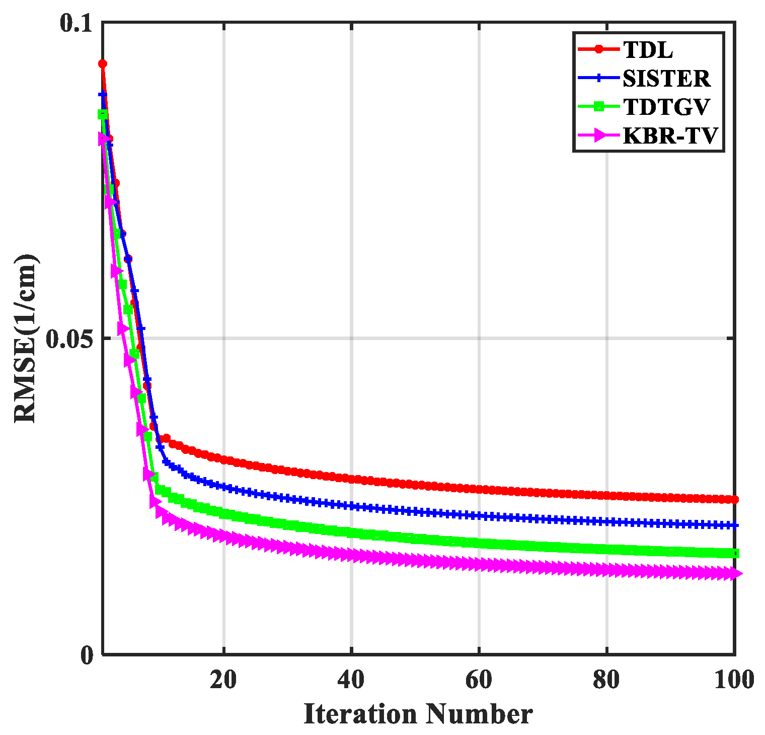
4.1. Numerical Simulation Study

In our numerical simulation study, a digital mouse thoracic model infused with a 1.2% iodine contrast agent was utilized to assess and contrast the performance of multiple reconstruction algorithms, as illustrated in Figure 2. The mouse model consists of three main components: soft tissue, bone, and iodine contrast. The X-ray source was configured to operate at 50 kVp, with its energy spectrum divided into eight distinct channels, as shown in Figure 3. An equidistant fan-beam scanning approach was employed during the experiment. Detailed parameters for the simulated data are provided in

Table 2. Detailed parameters for the simulated data.

Number	Parameter	Value
1	The distance between X-ray source and PCD	180 mm
2	The distance between X-ray source and rotation center	132 mm
3	The number of detectors	512
4	The size of detector element	0.1 mm
5	The size of image	256 × 256 × 8
6	The size of image pixel	0.15 mm

. A full 360° scan resulted in the acquisition of 640 projections; the noise distribution follows the Poisson distribution, with each X-ray path containing 5000 photons.

To validate the effectiveness of the proposed algorithm, reconstruction experiments with a projection angle of 160 were conducted. The reference image was generated by applying the FBP algorithm to noiseless projection data. In this experiment, two representative energy channels (1st channel and 8th channel) were selected for analysis. Figure 4 shows the reconstructed images using SART, TDL, SISTER, TDTGV, and the proposed algorithm KBR-TV. In the figure, the first two rows display the reconstruction results of channel 1 and channel 8, respectively, and the last two rows show the corresponding gradient images. From the figure, it can be seen that the KBR-TV algorithm proposed in this paper can obtain better quality reconstructed images. In particular, under low-dose and sparse-angle conditions, the SART algorithm, which does not incorporate prior knowledge, produces significant noise in the reconstructed image and shows the worst reconstruction quality. The TDL algorithm enhances image quality to a certain degree, but because of limitations in the quality of the tensor dictionary, it performs poorly in detail recovery. The SISTER and TDTGV algorithms further improve the quality of the reconstructed images, but still lose some small structures. In comparison, the KBR-TV algorithm demonstrates superior performance in restoring details and suppressing noise. As seen clearly in the last two rows of gradient images, the KBR-TV algorithm can recover more image details.

To further clearly illustrate the superiority of the KBR-TV algorithm and better compare the details of the reconstructed images, three regions of interest (ROIs) were identified in Figure 4a1, denoted as areas A, B, and C within the red dashed boxes. These regions were then enlarged to provide a closer examination of the reconstruction outcomes, as displayed in Figure 5. From the magnified regions, it is evident that the KBR-TV algorithm outperforms the others in reconstructing finer structural details, as highlighted by the red arrows. Specifically, in Figure 5a,b, the arrows “1”, “2”, “3”, and “4” indicate some small image structures that can be reconstructed by the KBR-TV algorithm, whereas they are lost in the other algorithms. Although in the TDTGV algorithm the structures indicated by arrows “2” and “3” can be reconstructed, they appear blurred. In contrast, the structures restored by the KBR-TV algorithm are clearer. From the gaps between bones indicated by arrows “5” and “6” in Figure 5c, it can be seen that the other algorithms reconstruct them rather vaguely, while the KBR-TV algorithm can reconstruct clearer structures, further demonstrating the superiority of the proposed method.

To compare the reconstruction accuracy of the algorithms, the yellow line regions in Figure 4a1 were selected to plot the gray-scale curves of the 1st and 8th channels, respectively, as shown in Figure 6. It can be observed from the figure that within the two energy spectrum channels, the reconstruction results of the KBR-TV algorithm proposed in this paper (red curve) are closer to the true values (black curve), indicating higher reconstruction accuracy.

In order to compare the performance of each algorithm numerically, three common metrics, RMSE, SSIM, and PSNR, were used for evaluation. Generally, reconstructed images are considered more accurate when they exhibit lower RMSE values and higher SSIM and PSNR values. The quantitative evaluations, as presented in

Table 3. Comparison of indicators by different methods.

Index	Method	1st	2nd	3rd	4th	5th	6th	7th	8th
RMSE (10−2)	SART	21.98	19.29	17.51	16.02	15.76	15.42	15.31	15.11
	TDL	12.51	10.79	8.97	8.65	7.76	6.34	4.14	2.39
	SISTER	10.34	9.11	7.58	7.12	6.28	5.57	3.14	1.87
	TDTGV	8.52	8.02	6.94	5.49	4.85	3.82	2.74	1.04
	KBR-TV	6.68	6.02	5.26	4.84	4.16	2.55	1.42	0.92
SSIM	SART	0.7867	0.7644	0.7210	0.6993	0.6873	0.6780	0.6518	0.6249
	TDL	0.9528	0.9548	0.9514	0.9508	0.9423	0.9311	0.9282	0.9235
	SISTER	0.9631	0.9600	0.9590	0.9577	0.9564	0.9526	0.9477	0.9406
	TDTGV	0.9740	0.9701	0.9686	0.9644	0.9576	0.9502	0.9496	0.9487
	KBR-TV	0.9836	0.9807	0.9814	0.9746	0.9735	0.9728	0.9717	0.9604
PSNR	SART	16.57	20.09	22.54	24.17	25.02	26.12	25.91	26.78
	TDL	25.38	28.03	30.57	33.72	32.43	34.75	37.67	40.02
	SISTER	30.72	34.21	37.82	39.01	40.07	41.43	41.96	43.12
	TDTGV	32.36	34.99	38.84	41.73	42.23	42.89	43.87	44.25
	KBR-TV	34.48	36.63	40.85	42.68	42.35	43.69	44.64	45.37

, demonstrate that the KBR-TV algorithm outperforms the others by achieving the best results across all three metrics. This indicates its superior reconstruction capability and further validates the effectiveness of the proposed approach.

Figure 7 presents a comparative evaluation of material-specific attenuation properties across eight channels to assess algorithmic reconstruction performance. The upper subfigures quantify relative bias between reconstructed and reference values for bone, soft tissue, and iodine contrast, while the lower subfigures depict channel-wise mean attenuation coefficients. Reference attenuation coefficients were derived through noiseless projection reconstruction using FBP as the ground-truth benchmark. From the figure, it can be seen that the KBR-TV algorithm achieves superior accuracy in material reconstruction across all energy channels compared to the other iterative reconstruction methods, further demonstrating the advantage of the algorithm proposed in this paper.

To compare the material component characterization capabilities of different algorithms, image domain-based material characterization algorithms were used to characterize the energy spectrum CT images reconstructed by SART, TDL, SISTER, TDTGV and KBR-TV algorithms; the reconstructions were characterized into three base materials: bone, soft tissue, and iodine contrast agent. Figure 8 shows the final image and the corresponding color image of the base material. The rows correspond to bone, soft tissue, iodine contrast agent, and their respective color representations after characterization. From Figure 8, the following conclusions can be drawn: For the bone region, the decomposition error of SART is the largest, followed by TDL. In the results of SISTER and TDTGV, some incorrect classifications of iodine contrast pixels can still be seen. In comparison, the bone image represented by the KBR-TV algorithm is clearer and achieves higher decomposition accuracy. For soft tissue, the KBR-TV algorithm can recover more fine lung structures, while other algorithms have blurred image structures. For iodine contrast agents, there are some errors in the comparison algorithms, but the KBR-TV algorithm achieves relatively accurate characterization.

In order to further quantitatively evaluate the material component characterization results,

Table 4. RMSE analysis for the decomposition of three fundamental components.

	Algorithm	Bone	Soft Tissue	Iodine Contrast
RMSE	SART	0.0894	0.1690	0.1029
	TDL	0.0282	0.0520	0.0311
	SISTER	0.0130	0.0423	0.0265
	TDTGV	0.0113	0.0408	0.0233
	KBR-TV	0.0092	0.0315	0.0207

shows the RMSE analysis results of each algorithm in the material component characterization. According to the table, the KBR-TV algorithm achieves the lowest RMSE value in the component characterization of the three base materials, showing high precision and accuracy, which further verifies the advantages of the algorithm.

To evaluate the convergence performance of the reconstruction methods, Figure 9 illustrates the RMSE trends of different algorithms with the number of iterations. As can be seen from the figure, the proposed algorithm in this paper converges faster and obtains the minimum RMSE value at the same time.

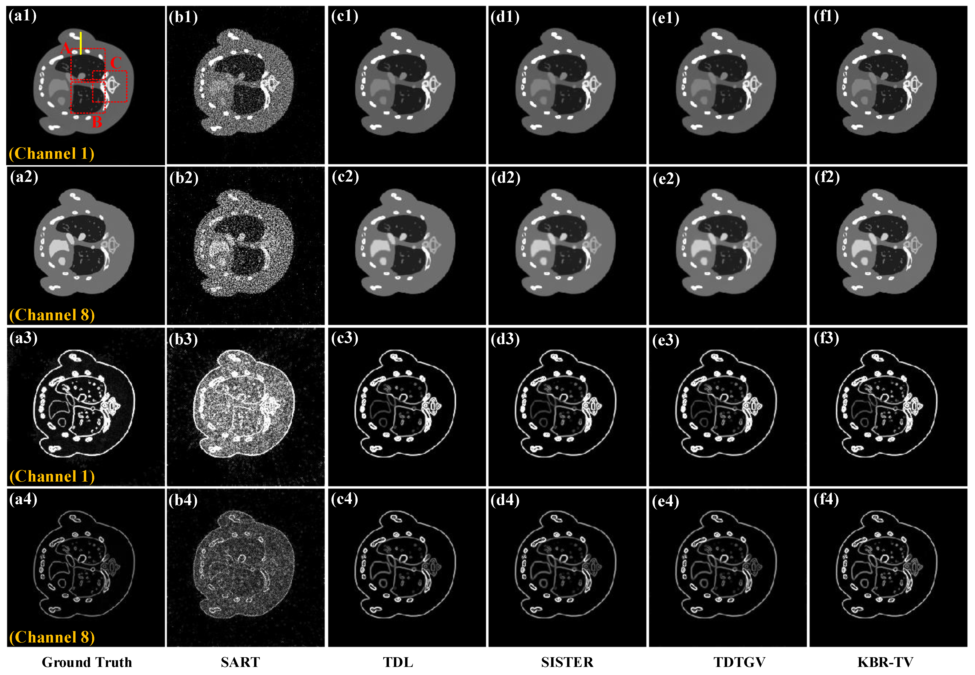
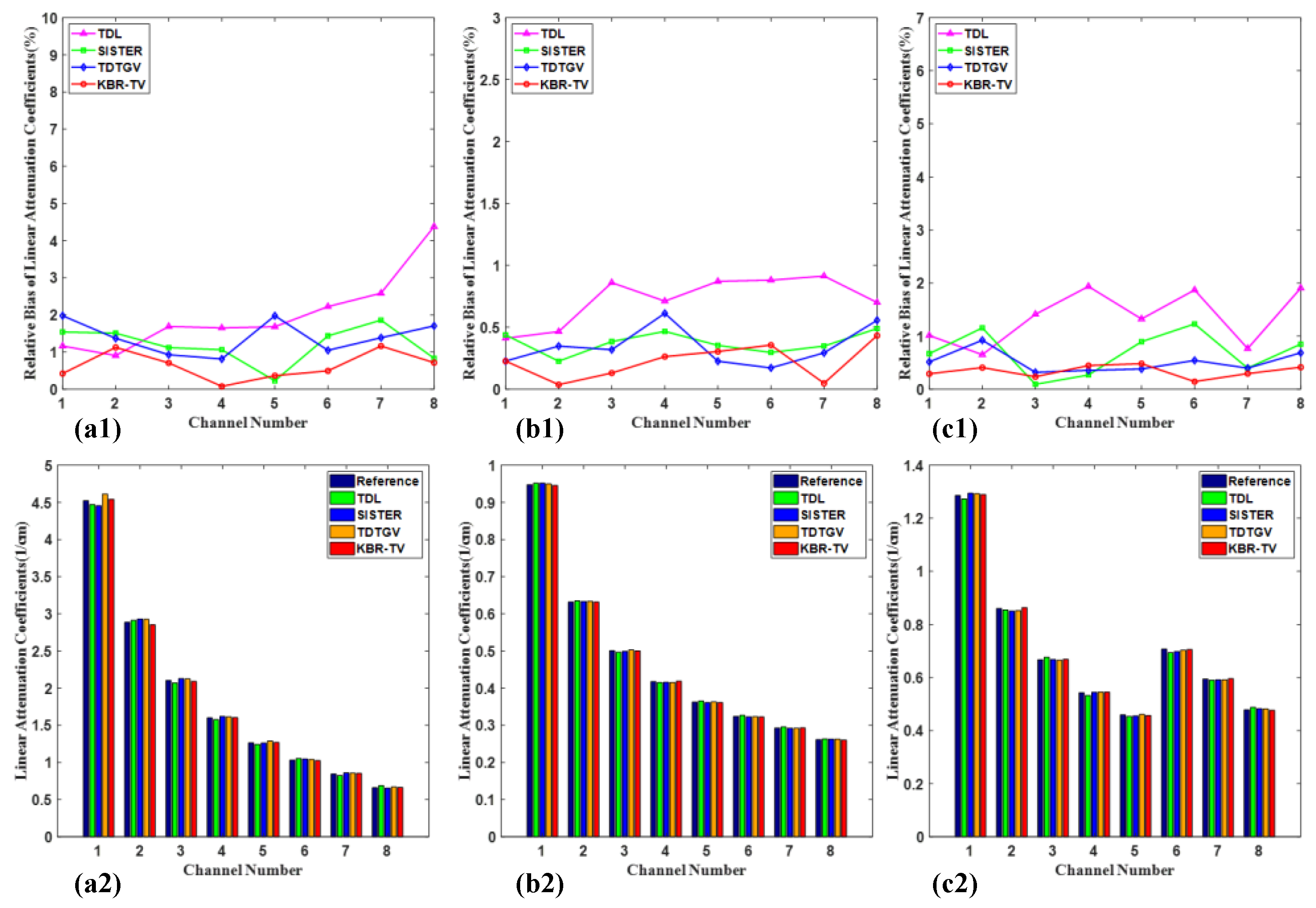
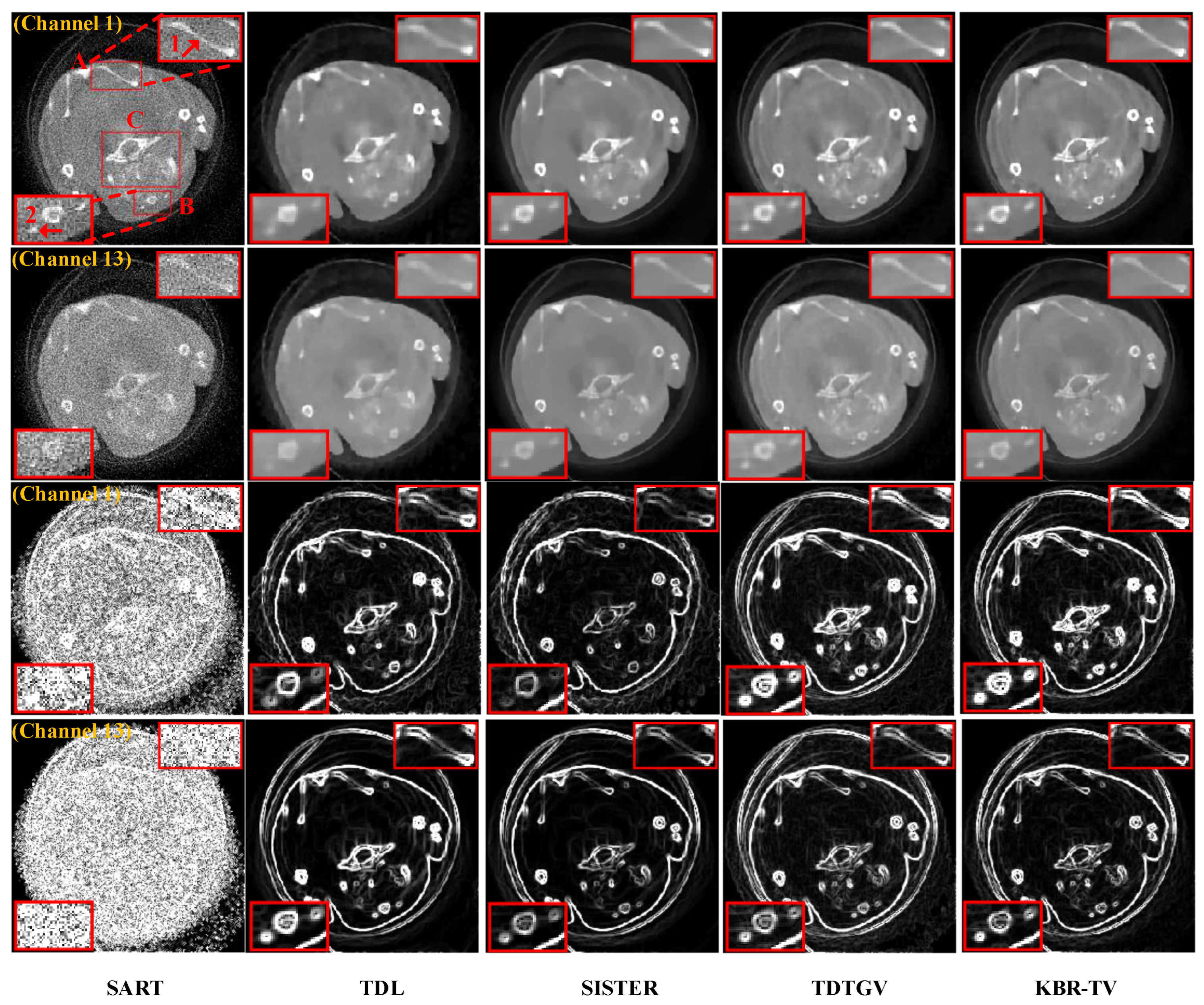
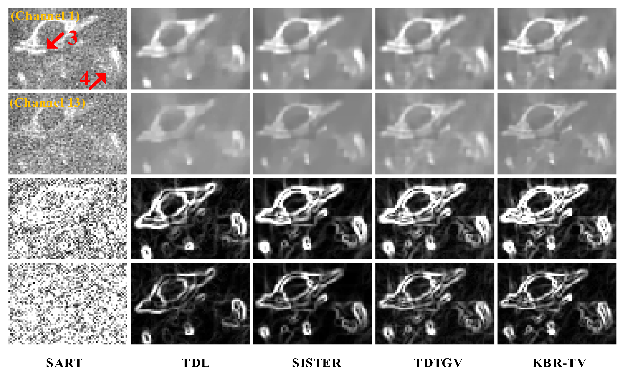
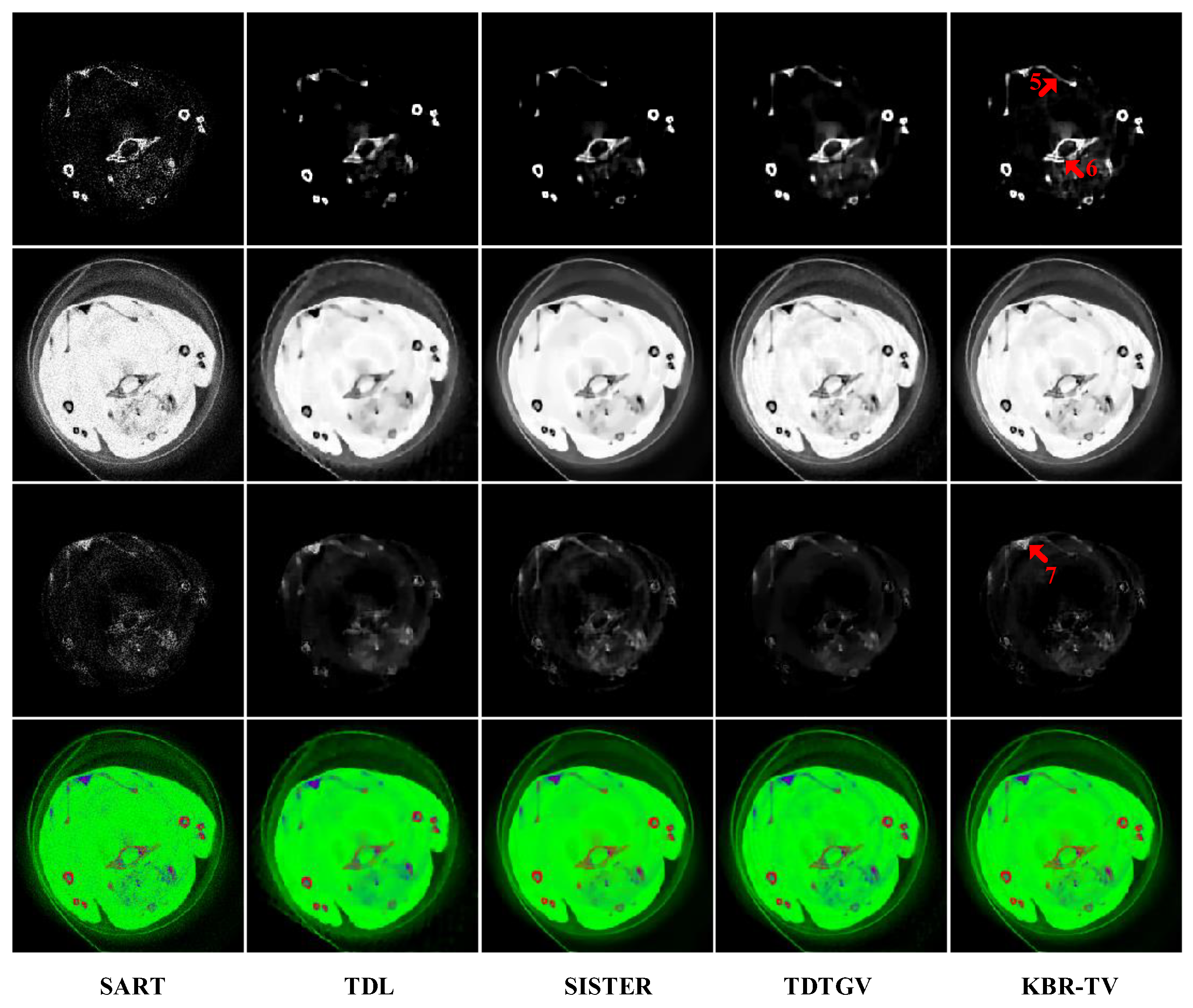
4.2. Actual Clinical Mouse Study

To further substantiate the effectiveness of the proposed KBR-TV algorithm, practical experiments were undertaken using a clinical mouse. In this study, a mouse injected with 0.2 mL of 15 nm Aurovist II gold nanoparticles (GNPs) (Nanoparticles; Yaphank, NY, USA) was utilized. The setup of the CT system includes an X-ray source operating at 120 kVp (divided into 13 energy channels) and a photon-counting detector. The photon-counting detector is a new type of sensor that combines CMOS technology and photon-counting technology. It can receive X-rays after passing through the mouse and obtain projection data of different energy channels simultaneously. During a complete scan, 371 projections were collected uniformly. Detailed parameters for the projection data acquisition are outlined in

Table 5. Detailed parameters for the projection data acquisition.

Number	Parameter	Value
1	The distance between X-ray source and PCD	255 mm
2	The distance between X-ray source and rotation center	158 mm
3	The number of detectors	512
4	The size of detector element	55 µm
5	The size of image	256 × 256 × 13

.

During this experimental procedure, image reconstruction was carried out using 120 projection views to assess the algorithm’s efficacy under conditions of sparse-view angles. In subsequent experiments, only two representative energy channels (channels 1 and 13) were presented for analysis. Figure 10 shows the reconstructed image using SART, TDL, SISTER, TDTGV, and the proposed KBR-TV algorithm. In the figure, the first two rows show the reconstruction results of channel 1 and channel 13, respectively, and the last two rows show the corresponding gradient images. As depicted in the figure, the SART algorithm yields the least satisfactory results, with pronounced noise and artifacts evident in the image, accompanied by significant loss of image structure. While the TDL algorithm offers an improvement in the quality of reconstructed images, it still suffers from structural blurriness. Both the SISTER and TDTGV algorithms markedly enhance image quality and restore finer details, yet they lag behind the KBR-TV algorithm in terms of restoring small image structures. This disparity becomes more apparent in the enlarged regions A and B extracted from the figure. The image structures indicated by arrows “1” and “2” are variously blurred in the comparison algorithms. In contrast, the image reconstructed using the KBR-TV algorithm is notably clearer, particularly in its superior restoration of small image structures, with this advantage being more pronounced in higher energy channels. The gradient images in the final two rows further demonstrate the clearer recovery achieved by the KBR-TV algorithm.

To further validate the advantages of the KBR-TV algorithm, a more complex region of interest (ROI C) was extracted from Figure 10 and enlarged for display in Figure 11. It becomes evident from the figure that the SISTER, TDTGV, and KBR-TV algorithms exhibit superior reconstruction performance. However, in comparison, the KBR-TV algorithm demonstrates an even better performance, as observed by the indicators pointed out by arrows. Specifically, the KBR-TV algorithm is capable of restoring clearer image structures, as indicated by arrows “3” and “4”. Notably, the gap between bones indicated by arrow “3” is more distinctly reconstructed by the KBR-TV algorithm, whereas other algorithms result in varying degrees of blurriness. The corresponding gradient images also support this conclusion in the last two rows.

To assess the material composition characterization capabilities of the algorithms, the spectral CT images reconstructed by different algorithms were characterized. Figure 12 presents the results of base material composition characterization along with the corresponding color images. The initial three rows show bone, soft tissue, and GNP (gold nanoparticle) components, respectively, while the fourth row shows the corresponding color representation (red for bone, green for soft tissue, and blue for GNP components). Red arrows “5”, “6”, and “7” indicate the characterized details. By observing the material decomposition results, the following conclusions can be drawn: In the bone region, it is evident that the TDTGV and KBR-TV algorithms obtain better bone images. These two algorithms can decompose the bone structure indicated by arrow “5”, which is missing in other algorithms. However, for the bone structure indicated by arrow “6”, the KBR-TV algorithm exhibits superior characterization, with clearer bone edges and a discernible gap between small bones. In the soft tissue region, the image obtained by the KBR-TV algorithm is smoother compared to those from other algorithms. Regarding GNP components, the accuracy of GNP obtained by the TDTGV and KBR-TV algorithms is similar. However, as seen from arrow “7”, the boundaries recovered by the KBR-TV algorithm are clearer. Overall, from the fused color images, the material composition characterization capability of the KBR-TV algorithm surpasses that of other reconstruction algorithms, yielding clearer images.

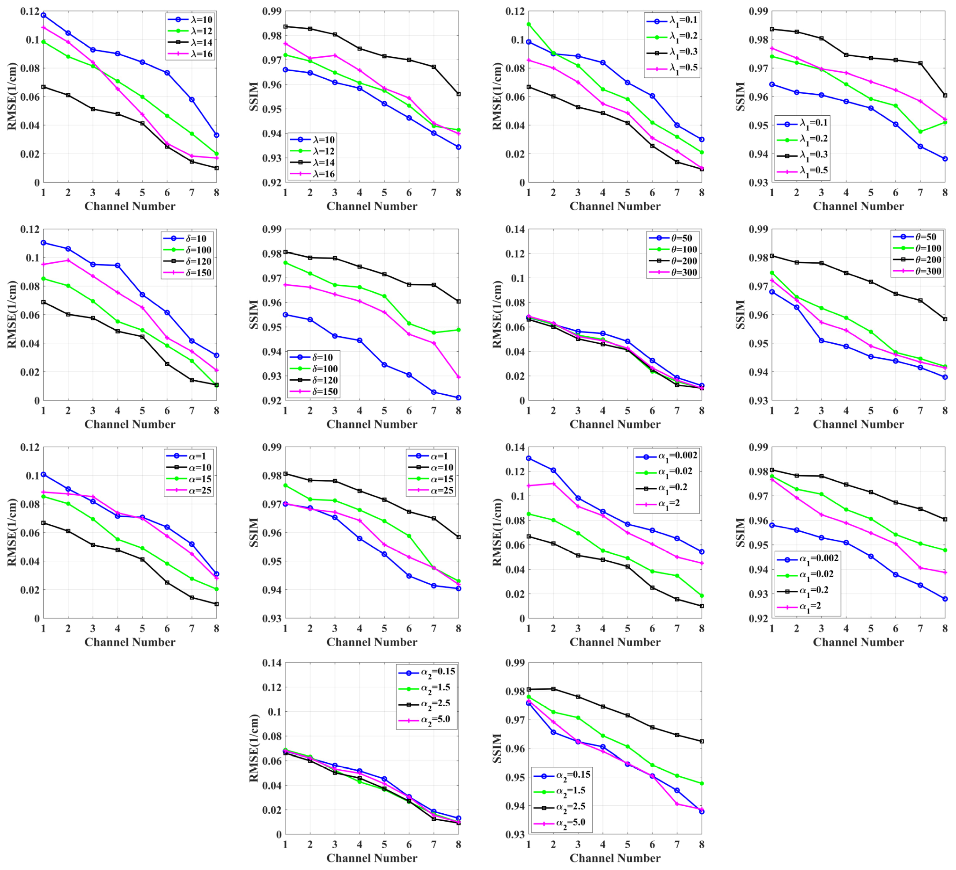
4.3. Parameter Analysis

The objective model defined in Equation (9) comprises two regularization terms with parameters to be optimized divided into two categories: the parameters for the KBR tensor decomposition term, primarily including λ, λ₁, δ, and θ, and the parameters for the TV regularization term, primarily comprising α, α₁, and α₂. The adjustment of these parameters exerts a considerable influence on the quality of images, and reconstructed images vary in quality based on various values. During the process of parameter selection, just one or two parameters are allowed to vary freely, with the remaining parameters held constant, and the image quality is experimentally assessed as it relates to these variable parameters. The selection of parameters is guided by the utilization of RMSE and SSIM values as evaluation metrics. It can be observed from the figure that the parameter values of λ, λ₁, and δ have a significant impact on the quality of the reconstructed images, with both excessively large and small values affecting image quality adversely. When set λ, λ₁, and δ to appropriate values, both RMSE and SSIM achieve optimal results. The coefficients α and α₁, associated with the two penalty terms in the TV regular term, also have a substantial influence on image quality. Setting these coefficients too low may introduce noise into the image, whereas excessively high values can lead to obvious smoothing of image edges. As illustrated in Figure 13, optimal settings for these coefficients result in the achievement of optimal RMSE and SSIM values. In comparison, θ and α₂ have minimal influence on the RMSE value of the reconstructed images. When θ and α₂ take different values, the resulting RMSE value is very close, but suitable values can significantly improve the SSIM value.

5. Discussion and Conclusions

To effectively utilize the inter-relationships between images captured across various energy channels, multispectral CT images collected by photon-counting detectors are typically transformed into a tensor model. By leveraging inherent properties like sparsity and low-rankness within the tensor, the reconstruction quality of spectral CT images is significantly improved. However, the traditional Tucker and CP tensor decomposition algorithms fail to unify low-rankness and sparsity in tensor space, compromising the quality of reconstructed images. To address this problem, this paper proposes a spectral CT image reconstruction algorithm that combines the KBR tensor decomposition with a TV regularization term. Firstly, by analyzing the mathematical expression of KBR, we theoretically verify that KBR tensor decomposition can unify traditional sparsity measures in tensor space while preserving more image structures. Subsequently, to eliminate image patch aggregation artifacts caused by intensity inconsistencies among pixels at the same positions, we introduce a TV constraint in the single energy channel. The introduction of the TV regularization term effectively reduces image patch artifacts and enhances image quality without excessively increasing the algorithm’s runtime. Finally, the split-Bregman method is employed to optimize and solve the reconstruction model. The experimental outcomes indicate that the proposed algorithm can improve the recovery of image structure, effectively suppress image block artifacts, and improve the accuracy of reconstruction.

Despite the positive outcomes achieved by the method, several challenges persist. Firstly, a significant number of parameters need to be determined. In this study, the selection of optimal parameters was carried out empirically, based on extensive experimental trials. Consequently, the challenge of automating the parameter optimization process remains unresolved and necessitates further investigation. Secondly, the weighting parameters (e.g., α, λ) across all energy channels are unified, which raises the concern that some channels may be over-regularized while others may be under-regularized. Therefore, it is necessary to explore an energy-channel-adaptive weighting scheme to improve reconstruction accuracy and robustness. Lastly, in practical applications, handling tensor volumes presents challenges due to their high computational demands and memory requirements. This paper undertakes a comparison of the runtime costs under uniform experimental conditions. Since the back-projection reconstruction times are consistent across all algorithms, our focus is solely on comparing the times associated with the regularization constraints. The runtime per iteration for each algorithm is presented in

Table 6. Computational costs of all methods (unit: seconds).

Methods	TDL	SISTER	TDTGV	KBR-TV
Running time	20.7 ± 1.1	40.5 ± 1.2	58.7 ± 1.6	120.6 ± 2.3

. As can be seen from the table, the KBR-TV algorithm consumes the longest calculation time due to its complexity in solving the model. Therefore, the introduction of a simple and effective TV regular term in the single-channel image domain can not only eliminate the block aggregation artifacts, but also ensure that the computation time does not increase much. Hence, further investigation and resolution of these issues are required, and they make up the main focus of our forthcoming research efforts.

In conclusion, this paper proposes a spectral CT image reconstruction algorithm that combines the KBR tensor decomposition with a TV regularization term. The proposed algorithm uses KBR tensor decomposition to replace the Tucker decomposition and CP decomposition in order to characterize the sparsity of the tensor and the low-rank properties of all expansion modes at the same time, achieving the consistency of the sparse metric of the traditional tensor space. In addition, to balance the low-rank property of space–energy spectrum domain and the sparsity of the spatial domain, a classical TV regularization term is introduced in the single energy channel. On the one hand, the introduction of TV can preserve more image structure; on the other hand, it can effectively reduce the artifacts in the single-channel image domain caused by the aggregation of tensor decomposition image blocks without excessively increasing the running time of the algorithm. The effectiveness of the proposed algorithm is verified by simulation experiments and a real mouse experiment.

References

1. Wang, G.; Yu, H.; De Man, B. An outlook on X-ray CT research and development. Med. Phys. 2008, 35, 1051–1064. [Google Scholar] [CrossRef]
2. Nakano, M.; Haga, A.; Kotoku, J.; Magome, T.; Masutani, Y.; Hanaoka, S.; Kida, S.; Nakagawa, K. Cone-beam CT reconstruction for non-periodic organ motion using time-ordered chain graph model. Radiat. Oncol. 2017, 12, 145. [Google Scholar] [CrossRef]
3. Brooks, R.A.; Di Chiro, G. Beam hardening in X-ray reconstructive tomography. Phys. Med. Biol. 1976, 21, 390–398. [Google Scholar] [CrossRef]
4. Zhao, W.; Li, D.; Niu, K.; Qin, W.; Peng, H.; Niu, T. Robust Beam Hardening Artifacts Reduction for Computed Tomography Using Spectrum Modeling. IEEE Trans. Comput. Imaging 2018, 5, 333–342. [Google Scholar] [CrossRef]
5. Kim, Y.; Kudo, H. Nonlocal Total Variation Using the First and Second Order Derivatives and Its Application to CT image Reconstruction. Sensors 2020, 20, 3494–3511. [Google Scholar] [CrossRef]
6. Nikzad, S.; Pourkaveh, M.; Vesal, N.J.; Gharekhanloo, F. Cumulative radiation dose and cancer risk estimation in common diagnostic radiology procedures. Iran. J. Radiol. 2018, 15, e60955. [Google Scholar] [CrossRef]
7. Greffier, J.; Frandon, J. Spectral photon-counting CT system: Toward improved image quality performance in conventional and spectral CT imaging. Diagn. Interv. Imaging 2021, 102, 271–272. [Google Scholar] [CrossRef]
8. Xi, Y.; Chen, Y.; Tang, R.; Sun, J.; Zhao, J. United Iterative Reconstruction for Spectral Computed Tomography. IEEE Trans. Med. Imaging 2015, 34, 769–778. [Google Scholar] [CrossRef]
9. Xu, Q.; Yu, H.; Bennett, J.; He, P.; Zainon, R.; Doesburg, R.; Opie, A.; Walsh, M.; Shen, H.; Butler, A.; et al. Image Reconstruction for Hybrid True-Color Micro-CT. IEEE Trans. Biomed. Eng. 2012, 59, 1711–1719. [Google Scholar] [CrossRef]
10. Xu, Q.; Yu, H.Y.; Mou, X.Q.; Zhang, L.; Hsieh, J.; Wang, G. Low-dose X-ray CT reconstruction via dictionary learning. IEEE Trans. Med. Imaging 2012, 31, 1682–1697. [Google Scholar] [CrossRef]
11. Xu, Q.; Liu, H.; Yu, H.; Wang, G.; Xing, L. Dictionary Learning Based Reconstruction with Low-Rank Constraint for Low-Dose Spectral CT. Med. Phys. 2016, 43, 3701. [Google Scholar] [CrossRef]
12. Zhao, B.; Ding, H.; Lu, Y.; Wang, G.; Zhao, J.; Molloi, S. Dual-dictionary learning-based iterative image reconstruction for spectral computed tomography application. Phys. Med. Biol. 2012, 57, 8217. [Google Scholar] [CrossRef]
13. Zhao, B.; Gao, H.; Ding, H.; Molloi, S. Tight-frame based iterative image reconstruction for spectral breast CT. Med. Phys. 2013, 40, 031905. [Google Scholar] [CrossRef]
14. Zeng, D.; Gao, Y.; Huang, L.; Bian, Z.; Zhang, H.; Lu, L.; Ma, J. Penalized weighted least-squares approach for multienergy computed tomography image reconstruction via structure tensor total variation regularization. Comput. Med. Imaging Graph. 2016, 53, 19–29. [Google Scholar] [CrossRef]
15. Wang, Q.; Salehjahromi, M.; Yu, H. Refined Locally Linear Transform-Based Spectral-Domain Gradient Sparsity and Its Applications in Spectral CT Reconstruction. IEEE Access 2021, 9, 58537–58548. [Google Scholar] [CrossRef]
16. Gao, H.; Yu, H.; Osher, S.; Wang, G. Multi-energy CT based on a prior rank, intensity and sparsity model (PRISM). INVERSE Probl. 2011, 27, 115012. [Google Scholar] [CrossRef]
17. Li, L.; Chen, Z.; Wang, G.; Chu, J.; Gao, H. A tensor PRISM algorithm for multi-energy CT reconstruction and comparative studies. J. Xray Sci. Technol. 2014, 22, 147–163. [Google Scholar] [CrossRef]
18. Rigie, D.S.; La Riviere, P.J. Joint reconstruction of multi-channel, spectral CT data via constrained total nuclear variation minimization. Phys. Med. Biol. 2015, 60, 1741–1762. [Google Scholar] [CrossRef]
19. He, Y.; Zeng, L.; Xu, Q.; Wang, Z.; Yu, H.; Shen, Z.; Yang, Z.; Zhou, R. Spectral CT reconstruction via low-rank representation and structure preserving regularization. Phys. Med. Biol. 2023, 68, 2996–3007. [Google Scholar] [CrossRef]
20. Zhang, Y.; Mou, X.; Wang, G.; Yu, H. Tensor-Based Dictionary Learning for Spectral CT Reconstruction. IEEE Trans. Med. Imaging 2017, 36, 142–154. [Google Scholar] [CrossRef]
21. Wu, W.; Zhang, Y.; Wang, Q.; Liu, F.; Chen, P.; Yu, H. Low-dose spectral CT reconstruction using image gradient ℓ0–norm and tensor dictionary. Appl. Math. Model. 2018, 63, 538–557. [Google Scholar] [CrossRef]
22. Li, X.; Sun, X.; Zhang, Y.; Pan, J.; Chen, P. Tensor Dictionary Learning with an Enhanced Sparsity Constraint for Sparse-View Spectral CT Reconstruction. Photonics 2022, 9, 35. [Google Scholar] [CrossRef]
23. Wang, M.; Hong, D.; Han, Z.; Li, J.; Yao, J.; Gao, L.; Zhang, B.; Chanussot, J. Tensor Decompositions for Hyperspectral Data Processing in Remote Sensing: A comprehensive review. IEEE Geosci. Remote Sens. Mag. 2023, 11, 26–72. [Google Scholar] [CrossRef]
24. Lin, J.; Huang, T.-Z.; Zhao, X.-L.; Ji, T.-Y.; Zhao, Q. Tensor Robust Kernel PCA for Multidimensional Data. IEEE Trans. Neural Netw. Learn. Syst. 2024, 36, 2662–2674. [Google Scholar] [CrossRef]
25. Osipov, D.; Chow, J.H. PMU Missing Data Recovery Using Tensor Decomposition. IEEE Trans. Power Syst. 2020, 35, 4554–4563. [Google Scholar] [CrossRef]
26. Zhang, S.; Guo, X.; Xu, X.; Li, L.; Chang, C.-C. A video watermark algorithm based on tensor decomposition. Math. Biosci. Eng. 2019, 16, 3435–3449. [Google Scholar] [CrossRef]
27. Peng, Y.; Meng, D.; Xu, Z.; Gao, C.; Yang, Y.; Zhang, B. Decomposable Nonlocal Tensor Dictionary Learning for Multispectral Image Denoising. In Proceedings of the 2014 IEEE Conference on Computer Vision and Pattern Recognition, Columbus, OH, USA, 23–28 June 2014; pp. 2949–2956. [Google Scholar]
28. Zhang, Y.; Salehjahromi, M.; Yu, H. Tensor decomposition and non-local means based spectral CT image denoising. J. Xray Sci. Technol. 2019, 27, 397–416. [Google Scholar] [CrossRef]
29. Hu, D.; Wu, W.; Xu, M.; Zhang, Y.; Liu, J.; Ge, R.J.; Chen, Y.; Luo, L.; Coatrieux, G. SISTER: Spectral-Image Similarity-Based Tensor with Enhanced-Sparsity Reconstruction for Sparse-View Multi-Energy CT. IEEE Trans. Comput. Imaging 2020, 6, 477–490. [Google Scholar] [CrossRef]
30. Wu, W.; Yu, H.; Liu, F.; Zhang, J.; Vardhanabhuti, V. Spectral CT reconstruction via Spectral-Image Tensor and Bidirectional Image-gradient minimization. Comput. Biol. Med. 2022, 151, 106080. [Google Scholar] [CrossRef]
31. Wang, S.; Wu, W.; Cai, A.; Xu, Y.; Vardhanabhuti, V.; Liu, F.; Yu, H. Image-spectral decomposition extended-learning assisted by sparsity for multi-energy computed tomography reconstruction. Quant. Imaging Med. Surg. 2023, 13, 610–630. [Google Scholar] [CrossRef]
32. Chen, X.; Xia, W.J.; Liu, Y.; Chen, H.; Zhou, J.L.; Zha, Z.Y.; Wen, B.H.; Zhang, Y. FONT-SIR: Fourth-Order Nonlocal Tensor Decomposition Model for Spectral CT Image Reconstruction. IEEE Trans. Med. Imaging 2022, 41, 2144–2156. [Google Scholar] [CrossRef]
33. Li, X.; Wang, K.; Xue, X.; Li, F. Sparse-View Spectral CT Reconstruction Based on Tensor Decomposition and Total Generalized Variation. Electronics 2024, 13, 1868. [Google Scholar] [CrossRef]
34. Wu, W.; Hu, D.; An, K.; Wang, S.; Luo, F. A High-Quality Photon-Counting CT Technique Based on Weight Adaptive Total-Variation and Image-Spectral Tensor Factorization for Small Animals Imaging. IEEE Trans. Instrum. Meas. 2021, 70, 2502114. [Google Scholar] [CrossRef]
35. Xie, Q.; Zhao, Q.; Meng, D.; Xu, Z. Kronecker-Basis-Representation Based Tensor Sparsity and Its Applications to Tensor Recovery. IEEE Trans. Pattern Anal. Mach. Intell. 2018, 40, 1888–1902. [Google Scholar] [CrossRef]
36. Xie, Q.; Zhao, Q.; Meng, D.; Xu, Z.; Gu, S.; Zuo, W.; Zhang, L. Multispectral Images Denoising by Intrinsic Tensor Sparsity Regularization. In Proceedings of the 2016 IEEE Conference on Computer Vision and Pattern Recognition (CVPR), Las Vegas, NV, USA, 27–30 June 2016; pp. 1692–1700. [Google Scholar]
37. Zeng, D.; Xie, Q.; Cao, W.; Lin, J.; Zhang, H.; Zhang, S.; Huang, J.; Bian, Z.; Meng, D.; Xu, Z.; et al. Low-Dose Dynamic Cerebral Perfusion Computed Tomography Reconstruction via Kronecker-Basis-Representation Tensor Sparsity Regularization. IEEE Trans. Med. Imaging 2017, 36, 2546–2556. [Google Scholar] [CrossRef]
38. Rudin, L.I.; Osher, S.; Fatemi, E. Nonlinear total variation based noise removal algorithms. Phys. D Nonlinear Phenom. 1992, 60, 259–268. [Google Scholar] [CrossRef]
39. Sidky, E.Y.; Pan, X. Image reconstruction in circular cone-beam computed tomography by constrained, total-variation minimization. Phys. Med. Biol. 2008, 53, 4777–4807. [Google Scholar] [CrossRef]
40. Gong, C.C.; Zeng, L. Self-Guided Limited-Angle Computed Tomography Reconstruction Based on Anisotropic Relative Total Variation. IEEE Access 2020, 8, 70465–70476. [Google Scholar] [CrossRef]
41. Du, X.S.; Kong, H.H.; Pan, J.X.; Qi, Z.W.; Li, J.X. Laplacian and bilateral weighted relative total variation sparse angle CT reconstruction. Phys. Scr. 2024, 99, 105212. [Google Scholar] [CrossRef]
42. Wu, J.F.; Wang, X.F.; Mou, X.Q.; Chen, Y.; Liu, S.G. Low Dose CT Image Reconstruction Based on Structure Tensor Total Variation Using Accelerated Fast Iterative Shrinkage Thresholding Algorithm. Sensors 2020, 20, 1647. [Google Scholar] [CrossRef]
43. Zhu, H.; Liu, X.X.; Huang, L.; Lu, Z.S.; Lu, J.; Ng, M.K. Augmented Lagrangian method for tensor low-rank and sparsity models in multi-dimensional image recovery. Adv. Comput. Math. 2024, 50, 75. [Google Scholar] [CrossRef]
Figure 1. Process of grouping the tensor. * represents the product of Nw and Nh.
Photonics 12 00492 g001
Figure 2. A digital mouse thoracic model used for the simulation. (a) Ground truth image; (b) iodine contrast; (c) material decomposition image: bone (red), soft tissue (green), iodine contrast (blue).
Photonics 12 00492 g002
Figure 3. The energy distribution of the X-ray source.
Photonics 12 00492 g003
Figure 4. Reconstructed images from different methods. From top to bottom, the display windows are [0, 0.25] cm−1, [0, 0.06] cm−1, [0, 0.03] cm−1, and [0, 0.03] cm−1, respectively.
Photonics 12 00492 g004
Figure 5. Magnified ROIs in Figure 4: (a) ROI A, (b) ROI B, and (c) ROI C.
Photonics 12 00492 g005
Figure 6. The intensity of the yellow line in Figure 4a1.
Photonics 12 00492 g006
Figure 7. The mean attenuation coefficients of three basic materials, bone (a1,a2), soft (b1,b2), and iodine contrast (c1,c2), and the corresponding relative bias.
Photonics 12 00492 g007
Figure 8. Material decomposition results: bone (red), soft tissue (green), and iodine contrast (blue). The display windows of 1st–3rd rows are [0, 0.1] cm−1, [0, 1] cm−1, [0, 0.5] cm−1.
Photonics 12 00492 g008
Figure 9. Convergence analysis of reconstruction algorithms.
Photonics 12 00492 g009
Figure 10. Reconstructed images by different methods. The display windows are [0, 0.08] cm−1 and [0, 0.008] cm−1, respectively.
Photonics 12 00492 g010
Figure 11. The magnification for ROI “C” in Figure 10.
Photonics 12 00492 g011
Figure 12. Material decomposition results: bone (red), soft tissue (green), and iodine contrast (blue). From top to bottom, the display windows are [0, 0.5] cm−1, [0, 1] cm−1, and [0, 1] cm−1, respectively.
Photonics 12 00492 g012
Figure 13. Quantitative examination of the reconstructed images with various parameters.
Photonics 12 00492 g013