Experimental Validation of Designs for Permeable Diffractive Lenses Based on Photon Sieves for the Sensing of Running Fluids

Abstract

This study reports the experimental validation of several designs of photon sieves with focusing capabilities. These permeable optical elements were implemented with a spatial light modulator working in pure-amplitude mode. The focal region was scanned using a traveling stage, holding a camera. Using this experimental setup, we characterized the focal region of the photon sieves and determined some parameters of interest, such as the depth of focus and the transverse extent of the focal region. These parameters and their evolution were measured and analyzed to compare the optical performance of different designs. Moreover, the permeability of the mask was also evaluated and is included in the discussion. When the photon sieve is intended to be used as an optical element for the monitoring of running fluids, one of the designs studied, labeled the Ring-by-Ring method, behaves in a quite balanced manner and thus has become the preferred choice. Through simulations for a refractometric sensor, we obtained the Figure of Merit of the Ring-by-Ring mask, which reached a maximum value of 7860 RIU⁻¹, which is competitive with plasmonic sensing devices.

1. Introduction

Long ago, diffractive optical elements (DOEs) found their place in the toolbox of optical designers [1,2,3,4]. They are typically realized as the amplitude and/or phase distributions on a plane, allowing for a compact and thin design on flat substrates. When focusing, collimation, or plane-to-plane image-forming capabilities are necessary, the sectorization of the DOE plane uses the classical Fresnel zone arrangement and generates the so-called Fresnel zone plates (FZPs) [5,6,7,8]. The detailed design of the FZPs strongly depends on the applicable manufacturing techniques and the type of modulation given by the element. Then, we can find the binary or multilevel amplitude and/or phase profiles, or even the polarization spatial distributions [9,10,11]. Unfortunately, the optical performance of DOEs and FZPs varies with the wavelengths of the operation, and most designs are specifically designed to work with monochromatic illumination. Moreover, FZPs are usually fabricated on non-permeable substrates. A permeable diffractive lens, such as that studied in this contribution, has several advantages: it is lighter because of the removal of material [12,13], and, more importantly, it allows for the passage of running fluids through it, enabling a low invasive implementation in ducts and tubes [14,15]. These types of DOEs are also called photon sieves (PSs). Another relevant field where PSs have found a very interesting niche is in X-ray optics. In this area, permeability is not an issue, and PSs are proposed because of their compactness and due to the lack of materials that require an index of refraction appropriate for the manufacturing of refractive lenses [16,17,18]. Also, THz optics have benefited from the implementation of photon sieves [19,20].

The practical realization of photon sieves opens apertures on a substrate or membrane. The open holes transmit both light and fluid, and the closed area obstructs or reflects the illumination, depending on the transmissive or reflective character or the PS, respectively. For transmission PSs, the substrate can be transparent, allowing for the generation of phase PSs when very thin membranes are used, or opaque. In the case of reflective PSs, the open zones cannot contribute to the reflected beam. In any case, the simplest PSs are binary DOEs, where the transmittance, reflectance, or phase can only take two values across their surfaces.

The limitations of the manufacturing technique used to fabricate PSs are of great importance when designing and optimizing the spatial distribution of apertures. In our approach, we only considered open apertures with a circular shape. The design of the PSs has to take into account the values of the radii that can be opened for a given substrate, the fabrication tools, and the testing constraints. Moreover, the distance between the adjacent apertures on the PSs should be large enough to prevent the coalescence of neighboring holes in order to maintain the substrate as topologically connected and to avoid collapse. Also, the aspect ratio of the holes is an important factor when permeability plays a significant role [21]. In our case, this aspect ratio is mostly determined by the substrate thickness and the fabrication method. Keeping all of this in mind, we propose several designs of feasible PSs. Our previous results were obtained with well-founded propagation algorithms to optimize and select the most promising designs. These simulations were conducted with a dedicated Python package called “Diffractio” [22]. Once the design is checked and validated through simulations, the next step is to mimic the actual optical behavior with an optical bench as an intermediate step before the real manufacturing of the PS. In fact, this study presents this intermediate experimental validation of the designs of three types of PSs and compares their behavior with the classical Soret lens (amplitude modulated binary FZP). We used a spatial light modulator (SLM), working in pure-amplitude modulation, to implement the spatial distribution of a PS working in transmission mode. SLMs have been previously used to analyze the optical behavior of complex DOEs with very good results [23]. Through using this approach, we avoid the cost and lead time of manufacturing a PS on a physical substrate. Therefore, the method used here can assist optical engineers when comparing designs, speeding up the validation stage. Additionally, we computationally simulated the same experiments to compare the results and to make a more robust analysis.

After this introductory section, we present (see Section 2) the PSs analyzed in this paper and how their specific layout was obtained and optimized. That section also contains a detailed description of the experimental setup used in this paper, as well as the definition of some parameters of interest that were extracted from the irradiance images collected in our experiment. Section 3 shows the results of a comparative analysis of the performance of the studied PS. This analysis was conducted using the parameters previously defined, and by keeping in mind the application of these elements in an optical system that can monitor optical parameters in a running fluid. This application, as a refractometric sensor, is exemplified with a photon sieve in Section 3. Finally, Section 4 summarizes the main findings of this study.

2. Materials and Methods

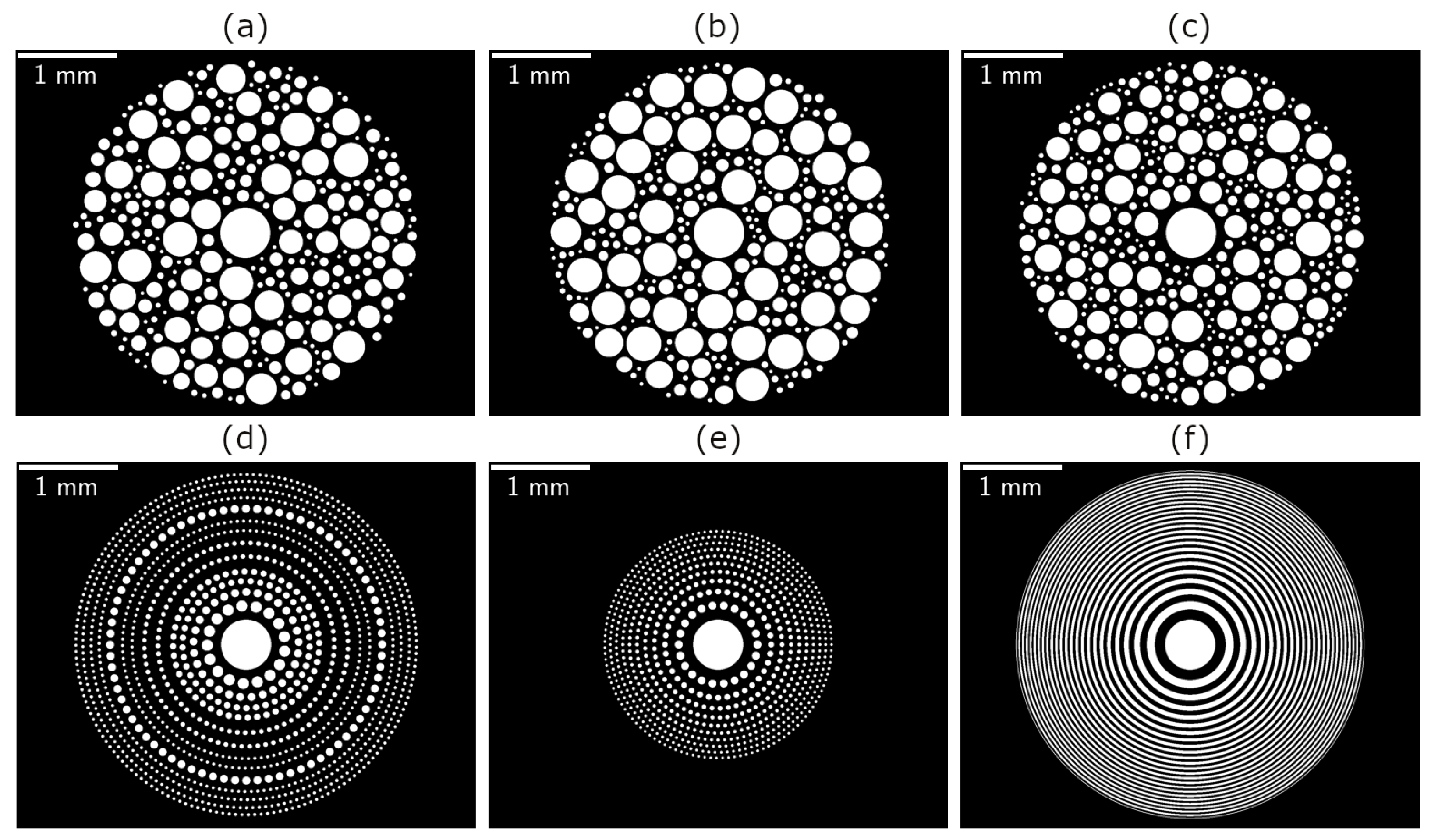
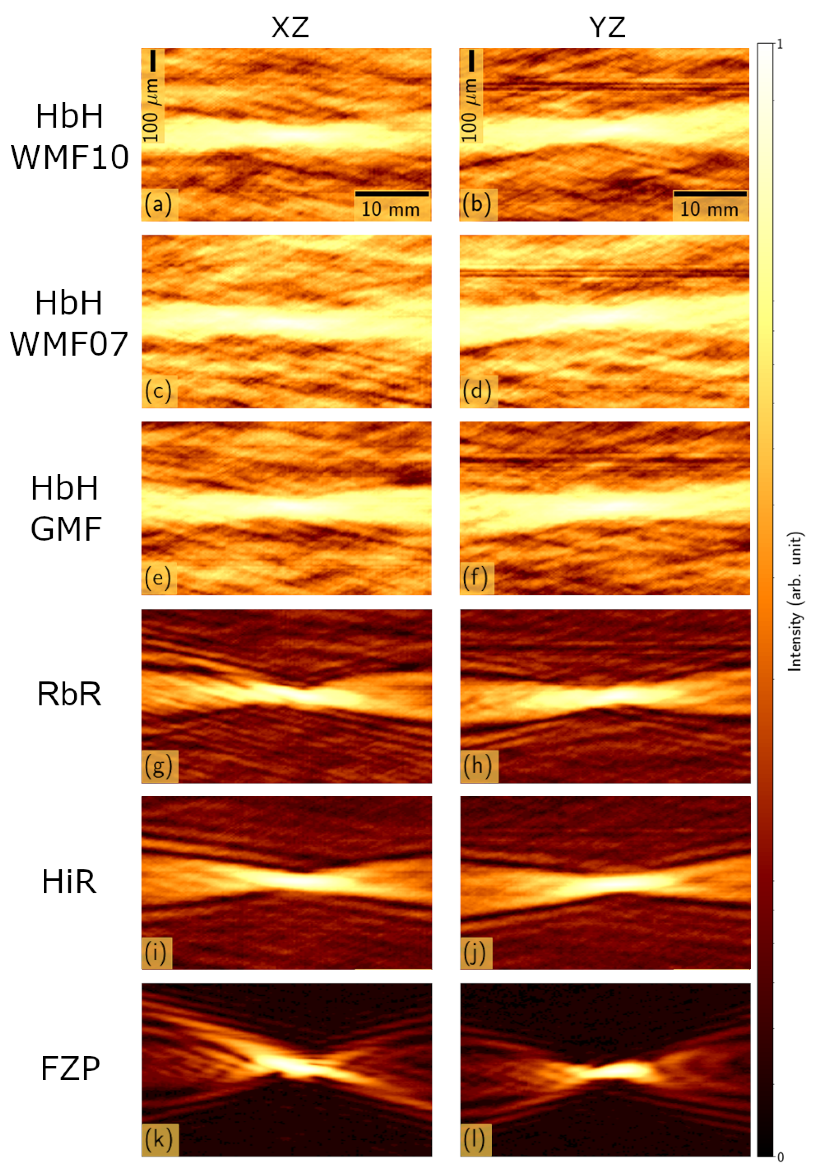
2.1. Types of Focusing Photon Sieves

The design process begins with selecting the focal length, $f^{\prime }$, of the photon sieve. For this study, we have set $f^{\prime }=100$ mm when operating in air. Additionally, for a diffractive optical element, we define the wavelength in vacuum, ${\lambda }_0=632.8$ nm, which is consistent with the wavelength used in our experimental characterization. These optical parameters determine the size of the central aperture, $r_1$, which is given by:

$$r_1=\sqrt{{\lambda }_0{f}^{\prime }}.$$

(1)

Another important constraint is the range of radii for the circular apertures in PS. The generation of permeable optical elements can be achieved using micromechanization methods or laser ablation. Previous studies have demonstrated that femtosecond laser ablation is both precise and flexible [24]. Therefore, in this analysis, we have considered the typical limitations associated with femtosecond laser ablation manufacturing. Practically, these constraints define the range for the radius of the apertures, which we have set in the interval $[16,180]$μm. The time required to fabricate numerous holes may compromise their accuracy in terms of location and shape. To address this issue, alternative manufacturing techniques such as chemical etching or attack can be employed to generate all the holes simultaneously, as demonstrated for various substrates and applications [25,26,27,28]. This approach is particularly important for the fabrication of wide-aperture photon sieves involving a large number of Fresnel zones.

Once the optical parameters of the lens were established, we considered three types of masks, each labeled according to the aperture generation method [29]. The Hole-by-Hole (HbH) masks are created iteratively, with each hole added consecutively. The location and size of each circular aperture are determined by an optimization algorithm [29,30]. This algorithm’s merit function balances the maximization of irradiance at the focal region and the permeability of the PS, evaluated based on the opened area. The upper row in Figure 1 displays three HbH masks generated in different runnings of the optimization algorithm and using two merit functions: Weighted Merit Function (WMF) and Geometric Merit Function (GMF). The WMF depends on the parameter w, which ranges from 0 to 1, indicating the importance of the irradiance at the focal region in the optimization. The mask labeled HbH WMF 1.0 (see Figure 1a) solely maximizes irradiance. In contrast, the mask HbH WMF 0.7 (Figure 1b) incorporates the permeability parameter with a 30% contribution (70% weight on irradiance), resulting in larger opened holes. The PS represented in Figure 1c uses a different merit function that balances the placement of new holes with the odd and even Fresnel zones. The Ring-by-Ring (RbR) mask generation algorithm, shown in Figure 1d, consecutively places equal-sized apertures in rings, selecting their location and size to maximize irradiance at the focal region. Figure 1e presents the Hole-in-Ring (HiR) mask, the simplest PS in this study. Circular holes are punched within the additive Fresnel zones, with diameters equal to the zone width. Manufacturing constraints exclude Fresnel zones with widths smaller than the minimum fabricable hole, reducing the number of apertures compared to other designs and limiting the aperture size. The classical FZP with the same focal length, $f^{\prime }=100$ mm, is shown in Figure 1f as a reference. It is important to note that this FZP is not a realizable PS because the closed regions are not connected and would collapse unless spokes are added, resulting in non-circular apertures. All masks presented in Figure 1 were experimentally validated and tested on the optical bench. The objective was to compare the predicted performance of these designs around the main focal point (first-order diffractional focus).

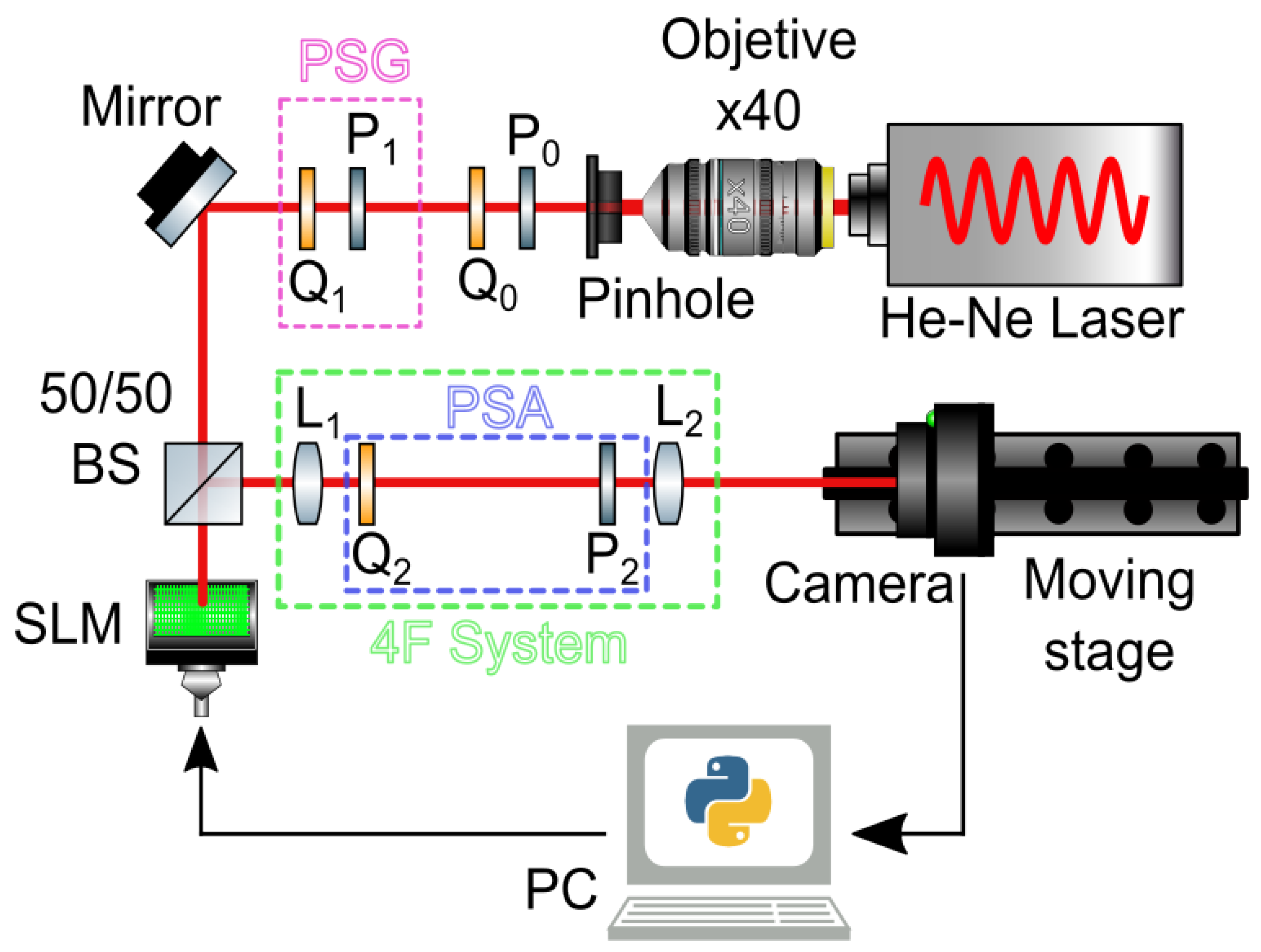
2.2. Experimental Setup

Figure 2 illustrates the experimental setup utilized in this study. The light source is a He-Ne laser (Melles Griot, United States) emitting a linearly polarized beam with a power of 10 mW. The laser beam is spatially filtered using a ×40 microscope objective and a 10 μm pinhole, resulting in a beam that fills the mask aperture. The key component of the setup is a spatial light modulator (SLM), model PLUTO-2.1 (Holoeye Photonics AG, Berlin, Germany). This device comprises a controller unit with a High-Definition Multimedia Interface (HDMI) and a single-phase Liquid Crystal on Silicon microdisplay with 8 μm square pixels and full-HD resolution (1920 × 1080 pixels). The SLM reduces the cost and time associated with manufacturing masks that fail to meet the minimum required specifications, while ensuring process reliability. Additionally, it facilitates the generation and test of various masks for comparative analysis. The SLM can operate in several modes: pure-amplitude, pure-phase, or mixed. In this study, we employed the pure-amplitude mode to generate an amplitude mask. This mode necessitates the preparation of the polarization state of the incoming beam and the observation of another specific polarization state. The Polarization State Generator (PSG), positioned between the laser source and the SLM, and the Polarization State Analyzer (PSA) are responsible for preparing these states. Both the PSG and PSA contain a linear polarizer (P₁ and P₂) and a quarter waveplate (Q₁ and Q₂). To ensure the SLM is illuminated under normal incidence conditions, a non-polarized 50/50 beam splitter (BS) is included to direct the reflection from the SLM towards the final measurement elements. The reflected light is collected by a 4$f^{\prime }$ optical system that produces a real image of the SLM plane with a lateral magnification of −1. This relay optical system consists of two lenses with focal lengths $f_1^{\prime }=f_2^{\prime }=10$ cm, with the PSA located between these lenses. Finally, the irradiance distribution on a plane perpendicular to the propagation axis is recorded by an IDS Imaging UI-1640LE-C-HQ camera. This camera features a 1.3-megapixel CMOS sensor with a resolution of 1280 ×1024 pixels and a square pixel size of 3.6 μm. The camera is mounted on a linear DC motor model M-ILS100CCL (Newport Corporation, Irvine, CA, USA), controlled by a single-axis motion controller SMC100CC (Newport Corporation). The movement resolution is 1 μm. By moving the camera, we can accurately scan the focal region with high spatial resolution along both the propagation axis and the transverse plane. The entire experiment is controlled by a dedicated Python package (under Python Kernel 3.10.8).

The initial step in this measurement involves fixing the orientation of the polarization elements of the PSG and PSA to ensure the SLM operates in a pure-amplitude configuration. This is achieved by adjusting the angles of these elements until the highest contrast is obtained in the image of a checkerboard object reproduced with the SLM. To accomplish this, the camera is placed at the image plane conjugated with the plane of the SLM through the $4f^{\prime }$ system. Once this condition is met, the PS mask is fed to the SLM, and the focal region is scanned by moving the camera along the Z-axis. Figure 3 displays the images obtained at the focal region for the RbR mask. Our PSs have a circular shape with a diameter of 3.5 mm, except for the HiR mask, which has a diameter of 2.3 mm due to fabrication constraints. After loading the mask onto the SLM, we verify that the image of the mask is registered by the camera. Subsequently, the camera is moved along the Z-axis to scan a 40 mm range around the focal plane position ($f^{\prime }=100$ mm) with a step length of 0.3 mm. For each mask, the gain and integration time of the camera are adjusted to maximize the available dynamic range of 256 gray levels.

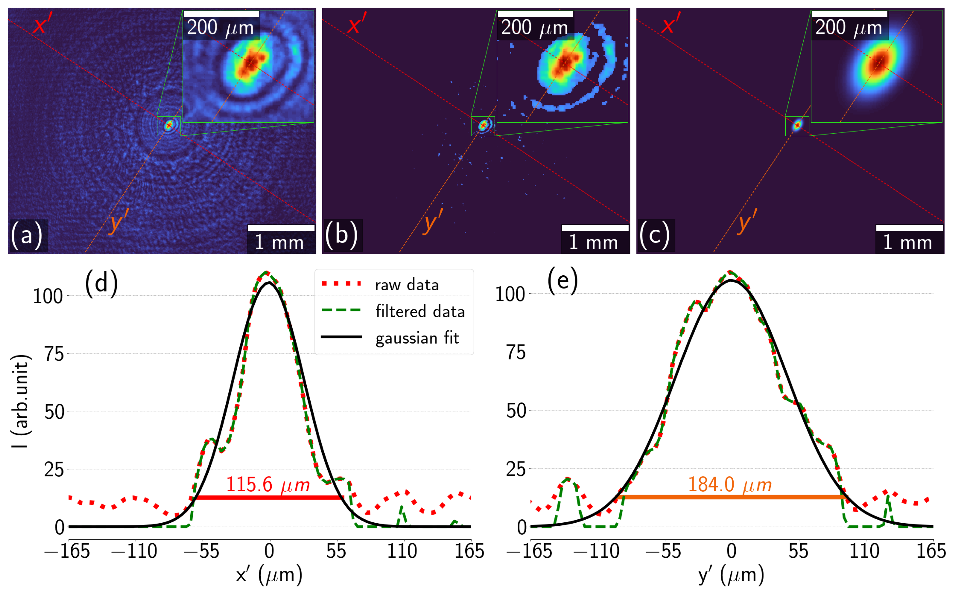
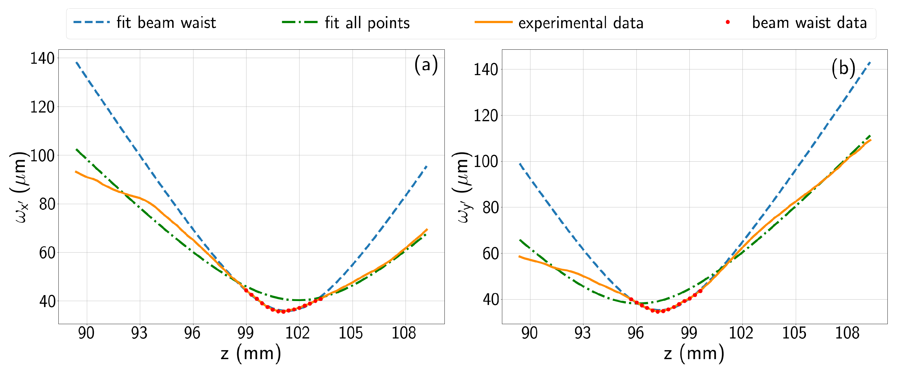
2.3. Parameterization of the Focal Region and Mask

Figure 3a–c presents images captured at three planes around the focal plane at $z=89$, 100, and 107 mm for the RbR PS. The irradiance distribution exhibits an elliptical cross-section, likely resulting from misalignment within the optical train or residual, uncorrected phase aberrations of the SLM. This astigmatism is more accurately characterized using a generalized measure of ellipticity defined as

$$\widehat{\eta }={\displaystyle \frac{a-b}{\sqrt{ab}}},$$

(2)

where a and b are the semi-axes of the ellipse, and $\sqrt{ab}$ represents the geometric mean of these semi-axes, corresponding to the radius of a circle with the same area as the ellipse. From Figure 3d, we observe that the ellipticity is zero around $z\approx 99.4$ mm. This location corresponds to the change in the orientation of the major axis of the ellipse and should coincide with the nominal focal distance, $f^{\prime }=100$ mm. The observed small discrepancy may arise from a slight deviation in the lateral magnification value of the $4f^{\prime }$ system, which should be $-1$.

The performance of the PS in optical sensing applications depends on its focalization and collimation capabilities. To accurately characterize these properties, we have analyzed the lateral and axial extension of the focal region obtained for a given PS when illuminated by a plane wave. Specifically, we have evaluated the depth of focus (DOF) and the beamwidth transversal size. For a laser beam, it has been demonstrated that when the DOF is defined in terms of the Rayleigh range, there exists an analytical relationship between the transversal and longitudinal extent of the waist [31]. Following the laser beam propagation model, we have also calculated the beam quality factor, $M^2$. Additionally, other geometrical parameters of the propagation and the mask, such as the beam’s ellipticity and the device’s permeability, have been evaluated. The latter quantity, defined subsequently, determines the permeability of the PS and how the device manages the presence of running fluids.

The experimental analysis of the DOF utilizes the axial irradiance evolution, evaluated by measuring the maximum irradiance value at each plane along the Z axis. Figure 4 illustrates the case of the RbR PS, where the axial normalized irradiance is plotted against the z coordinate. The irradiance reaches its peak around the nominal focal distance, $z=f^{\prime }=100$ mm. We characterize the axial extent of this peak using the Full Width at Half Maximum (FWHM) of the z evolution of the normalized irradiance. To determine this FWHM, we subtract the minimum value of this evolution, which is 0.2, resulting in the half maximum appearing at a level of 0.6 (see Figure 4). The DOF obtained from this criterion is considered a coarse estimation of the focal region of the photon sieve. Given that the distance between consecutive planes is 300 μm, we adopt this value as the experimental uncertainty of this parameter.

Due to the non-uniformities in the irradiance distribution observed with the camera, evaluating the transversal size requires dedicated image analysis. Figure 5 illustrates the method employed in this study. We start with the raw image, presented in Figure 5a as an irradiance map, with the center detailed in an inset. To properly isolate and provide a reliable value for the transversal size of the beam, we applied a filter to the original image. This filter zeroes every pixel with a value lower than a specified threshold. The selection of this threshold is based on the histogram of the entire image, ensuring the preservation of values around the maximum irradiance. Figure 5b shows the irradiance map after this preprocessing step. The resulting map is then fitted to a Gaussian distribution of irradiance, and the parameters of this fitting are used to characterize the transversal shape. However, as seen in the insets of Figure 5 (and also in Figure 3), the beam exhibits an elliptical shape oriented along a new set of rotated axes $X^{\prime }$, $Y^{\prime }$, with a rotation angle $\alpha =-34.1^{\circ }$. Therefore, the fitting of the irradiance distribution is performed using the following 2D Gaussian beam function:

$$f(x^{\prime },y^{\prime })=Aexp\left\{-2\left[{\displaystyle \frac{{(x^{\prime }-x_0^{\prime })}^2}{w_{x^{\prime }}^2}}+{\displaystyle \frac{{(y^{\prime }-y_0^{\prime })}^2}{w_{y^{\prime }}^2}}\right]\right\},$$

(3)

where $x^{\prime }$ and $y^{\prime }$ are the coordinates with respect to the rotated axis frame, $(x_0^{\prime },y_0^{\prime })$ is the location of the beam center, and ${\omega }_{x^{\prime }}$, ${\omega }_{y^{\prime }}$ are the Gaussian widths of the electric field distribution associated with the modeled beam along the $X^{\prime }{Y}^{\prime }$ axis. The irradiance distribution for this ideal Gaussian distribution is shown in Figure 5c. This fitting is depicted in Figure 5d and Figure 5e along the two rotated axes $X^{\prime }$ and $Y^{\prime }$, respectively. An alternative approach to determine the transversal size could involve using the FWHM. However, this parameter is more susceptible to local irradiance variations than the Gaussian fitting. Moreover, for a Gaussian profile, there is a direct relationship between the Gaussian width of the amplitude distribution $\omega$ and the FWHM:

$$\mathrm{F}\mathrm{W}\mathrm{H}\mathrm{M}=\omega \sqrt{2ln2}.$$

Once the fitting is performed for each transversal plane, we compare this evolution with a Gaussian beam propagation model, which can be expressed as:

$$\omega \left(z\right)={\omega }_0\sqrt{1+{\left({\displaystyle \frac{z-z_0}{z_R}}\right)}^2},$$

(4)

where ${\omega }_0$ is the Gaussian beam width at the beam’s waist plane, and $z_R$ is the Rayleigh range of the beam, which also measures the axial extent of the waist. Additionally, the previous fitting determines the beam’s evolution in regions farther from the beam waist. This propagation can be characterized by the beam’s divergence, which, for a Gaussian beam, is mathematically defined as

$${\theta }_0=\underset{z\to \infty }{lim}{\displaystyle \frac{\omega (z-z_0)}{z-z_0}}={\displaystyle \frac{{\omega }_0}{z_R}}.$$

(5)

The previously defined parameters of minimum width, ${\omega }_0$, and divergence, ${\theta }_0$, can be derived from the evolution of the Gaussian widths, $\omega \left(z\right)$, evaluated from the irradiance maps. In Figure 6, the experimental values of the Gaussian widths are plotted as orange dots. We then model this evolution using Equation (4), with ${\omega }_0$, $z_R$, and $z_0$ as fitting parameters. The results differ significantly when considering all the experimental data (see green dotted line in Figure 6) versus only the points around the focal region (see blue dashed line in Figure 6). The fitting with all points better reproduces the divergence (though it overestimates the minimum width), while the fitting with only the central points better matches the focal region values (though it overestimates the divergence). At this point, we utilize the laser beam quality parameter $M^2$, defined as [32]:

$$M^2={\displaystyle \frac{\pi {\omega }_0{\theta }_0}{\lambda }},$$

(6)

which encapsulates the beam’s quality in a single dimensionless variable, with the ideal Gaussian beam having a value of $M^2=1$. In our case, we take ${\omega }_0$ as the fitted value for the minimum width, ${\omega }_0$, in Equation (6) when considering only the central points, and ${\theta }_0$ is obtained from the fitting with all values, after applying Equation (5).

Finally, for each mask analyzed in this study, we evaluate the permeability parameter ${\widehat{A}}_{\mathrm{PS}}$, defined as

$${\widehat{A}}_{\mathrm{PS}}={\displaystyle \frac{A_{\mathrm{open}}}{A_{\mathrm{FZP}}}},$$

(7)

where $A_{\mathrm{open}}$ is the area of the open circles, and $A_{\mathrm{FZP}}$ corresponds to the open area of a classical Soret FZP.

3. Results and Discussion

To compare the performance of the masks implemented in the SLM (see Figure 1), we conducted both experimental validations and simulations of the elements. The input amplitude was propagated through the masks using the Chirped Z-Transform algorithm [33,34,35], implemented within the Python module “Diffractio” [22]. The transversal irradiances obtained from these simulations were analyzed using the same parameters as those used in the experimental validation.

Table 1. Experimental (in upright font) and computational (in italics) values of the characterizing parameters for the studied masks. The FZP column is considered to be the reference.

HbH WMF 1.0	HbH WMF 0.7	HbH GMF	RbR	HiR	FZP
DOF [mm]
$9.2\pm 0.4$	$13.9\pm 0.4$	$8.9\pm 0.4$	$8.7\pm 0.4$	$10.3\pm 0.4$	$10.4\pm 0.4$
10.9 ± 0.4	10.6 ± 0.4	11.8 ± 0.4	9.0 ± 0.4	8.9 ± 0.4	5.3 ± 0.4
${\omega }_{0,x^{\prime }}$ [μm]
$46.5\pm 0.4$	$48.0\pm 0.4$	$68.5\pm 0.3$	$35.9\pm 0.2$	$33.4\pm 0.2$	$24.8\pm 0.4$
9.80 ± 0.05	60.96 ± 0.09	48.88 ± 0.03	33.5 ± 0.2	32.91 ± 0.04	24.25 ± 0.03
${\omega }_{0,y^{\prime }}$ [μm]
$57.0\pm 0.4$	$60.2\pm 0.4$	$51.9\pm 0.2$	$35.1\pm 0.2$	$31.5\pm 0.1$	$22.9\pm 0.5$
52.05 ± 0.05	53.50 ± 0.07	59.86 ± 0.03	33.5 ± 0.2	32.91 ± 0.04	24.25 ± 0.03
$\mathrm{\Delta }{z}_{f^{\prime }}$ [mm]
$1.7\pm 0.1$	$1.1\pm 0.2$	$0.1\pm 0.1$	$3.99\pm 0.04$	$5.40\pm 0.03$	$4.56\pm 0.05$
0.16 ± 0.02	0.02 ± 0.04	0.38 ± 0.02	0.00 ± 0.03	0.00 ± 0.02	0.00 ± 0.01
${\widehat{\eta }}_{f_t}(1\times {10}^{-3})$
$-64\pm 2$	$-153\pm 3$	$307\pm 3$	$-157.6\pm 0.7$	$-61.9\pm 0.2$	$-242.6\pm 0.5$
136 ± 2	192.6 ± 0.2	−204.1 ± 0.1	−0.09 ± 0.03	−0.07 ± 0.03	−0.00 ± 0.01
$M_{x^{\prime }}^2$
$1.34\pm 0.04$	$1.17\pm 0.03$	$2.45\pm 0.04$	$1.34\pm 0.04$	$1.38\pm 0.02$	$1.7\pm 0.5$
1.79 ± 0.01	1.87 ± 0.03	1.63 ± 0.01	1.27 ± 0.01	1.32 ± 0.02	1.09 ± 0.03
$M_{y^{\prime }}^2$
$1.85\pm 0.07$	$1.96\pm 0.06$	$1.47\pm 0.01$	$1.39\pm 0.04$	$1.26\pm 0.03$	$1.5\pm 0.5$
1.49 ± 0.02	1.72 ± 0.02	1.86 ± 0.02	1.28 ± 0.01	1.32 ± 0.02	1.09 ± 0.03
${\widehat{A}}_{\mathrm{PS}}$ [%]
$98.24\pm 0.01$	$110.33\pm 0.01$	$94.08\pm 0.01$	$43.80\pm 0.01$	$21.80\pm 0.01$	$100\pm 0.1$

presents the values derived from the experiments (in upright font) and the simulations (in italic font). In this analysis, the classical Soret lens (FZP) was used as a reference. Additionally, we performed an uncertainty evaluation for each variable, calculated as follows:

$$\mathrm{\Delta }U\left(x_1,x_2,\dots ,x_m\right)=\sqrt{\sum _{i=1}^m\left[{\left({\displaystyle \frac{\partial U}{\partial x_i}}\right)}^2{\left(\mathrm{\Delta }{x}_i\right)}^2\right]}.$$

(8)

In this context, U represents any of the aforementioned quantities, while $x_i$ denotes the independent variables, each associated with an uncertainty $\mathrm{\Delta }{x}_i$. An exception to this is the uncertainty in the depth of focus (DOF), which is related to the resolution of the moving stage.

In addition to the results presented in Table 1, the optical behavior around the focal plane can be further analyzed by examining the propagation of light along the axis, as illustrated in Figure 7. This figure presents the irradiance map on two perpendicular planes containing the propagation axis: $XZ$ and $YZ$. In these plots, a logarithmic representation normalized to the maximum value for each mask is used. These visualizations demonstrate how light is focused in the focal region or distributed around it for each mask.

As demonstrated, the DOF values (see Figure 4) are crucial for determining the optimal placement of a detector within the focal region along the Z-axis. When comparing the experimental values in Table 1, it is evident that the minimum DOF is observed for the RbR mask. However, simulations indicate that the shortest DOF is produced by the FZP mask, with the RbR mask being the most effective among those with the same aperture as the FZP mask (due to fabrication constraints, the aperture of the HiR mask has been limited as shown in Figure 1e). The significant discrepancies between the experimental and simulated DOF values for the FZP mask are likely due to irradiance variations in our experimental images. Regarding the width values, ${\omega }_{0x^{\prime }}$ and ${\omega }_{0y^{\prime }}$, it is important to note that these are calculated along the rotated axes $X^{\prime }$ and $Y^{\prime }$, which align with the main axis of the elliptical irradiance distribution. The observed discrepancy between ${\omega }_{0x^{\prime }}$ and ${\omega }_{0y^{\prime }}$ in the measured images is attributed to astigmatism in our experimental setup, likely caused by residual phase aberrations at the SLM. For completeness, we have calculated $\mathrm{\Delta }{z}_{f^{\prime }}=|z_{f_{x^{\prime }}^{\prime }}-z_{f_{y^{\prime }}^{\prime }}|$ to quantify the axial distance between the orthogonal beam waists for each PS design. The simulation results show that $\mathrm{\Delta }{z}_{f^{\prime }}$ is zero for masks with axial symmetry (RbR, HiR, and FZP), whereas the HbH mask exhibits a non-zero value due to its lack of symmetry. Conversely, the experimental values of $\mathrm{\Delta }{z}_{f^{\prime }}$ are smaller for the HbH masks, indicating that the astigmatism induced by the SLM is more pronounced for axially symmetric masks. A similar trend is observed for ${\widehat{\eta }}_{f_t^{\prime }}$. The previously defined beam quality factor $M^2$, given in Equation (6), reaches its minimum value for the RbR and HiR masks, indicating that the focal region performs well for these masks. Due to the definition of $M^2$ in this study, which uses two different fittings to obtain ${\omega }_0$ and ${\theta }_0$, the value of $M^2$ should be considered an underestimation. Nonetheless, the large experimental $M^2$ value for the FZP mask is primarily due to our method of evaluating Gaussian widths and the aforementioned residual astigmatism at the SLM. In contrast, the $M^2$ value calculated through simulations is lowest for the FZP mask, as expected, with the RbR mask following closely. When considering only simulations, $M_x^2=M_y^2$ for masks with rotational symmetry around the optical axis Z. The permeability values presented in Table 1 are directly referenced to the FZP mask, as defined in Equation (7). As anticipated from the generation methods, the HbH WMF 0.7 design exhibits the highest permeability, while the HiR design shows the lowest. This is because the former prioritizes the open area of the lens, whereas the latter is constrained by its aperture size.

Examining the axial irradiance distribution in Figure 7 reveals that the FZP mask performs the best at focusing light around the focal region. Unfortunately, this FZP mask is not feasible as a PS and should be discarded. Transforming this FZP into a topologically connected PS can be achieved using radial spokes; however, this approach involves non-circular open apertures, which have not been considered in this analysis. In terms of DOF, the HbH WMF 0.7 mask produces the longest focal region. Additionally, this mask generates a relatively wide focal region and distributes a significant amount of light outside it (see the second row in Figure 7), resulting in a weaker optical signal. Conversely, the HbH WMF 0.7 mask has the highest permeability parameter ${\widehat{A}}_{\mathrm{PS}}$, as expected for a mask designed to maximize the open area of the PS. The other two HbH masks also exhibit an irradiance distribution with substantial light outside the focal region, likely due to the seemingly random distribution of holes. When considering the width of the focal region, indicated by the ${\omega }_{0,x^{\prime }}$ and ${\omega }_{0,y^{\prime }}$ parameters, the HiR mask performs the best. However, this mask has the smallest aperture due to the limitation of the fabricable radius of the open circles. This small aperture also corresponds to a lower optical signal at the focal plane and explains why the permeability parameter ${\widehat{A}}_{\mathrm{PS}}$ is the smallest in our analysis. The RbR mask appears to offer a more balanced performance. It demonstrates better behavior in terms of irradiance distribution (see Figure 7), with intermediate values for DOF and widths. Additionally, the permeability parameter is about half that of the FZP, lower than the HbH masks, and approximately twice the value for the HiR PS.

The previous analysis, based on Table 1 and Figure 7, aids in making an informed choice for a specific application. One such application of PS is to obtain an optical signal when light propagates through running fluids crossing the mask [30]. For the case discussed in the next subsection, the preferred element should generate a high irradiance around the focal region where the detection system is to be placed, with significant variation when moving axially, indicating a short DOF with ${\omega }_0$ as small as possible. Simultaneously, as an element inserted within a running fluid, high permeability is desired. Topologically, the FZP cannot be considered a PS. Optically, all HbH masks distribute excessive light outside the focal region. This behavior is due to the lower axial symmetry of these designs compared to others (see Figure 1). Consequently, the RbR and HiR designs, which have similar spot size and shape, are the most suitable proposals for our case. As a tiebreaker between these two options, if larger permeability and aperture (allowing more light to pass through) are preferred, the RbR mask would be selected.

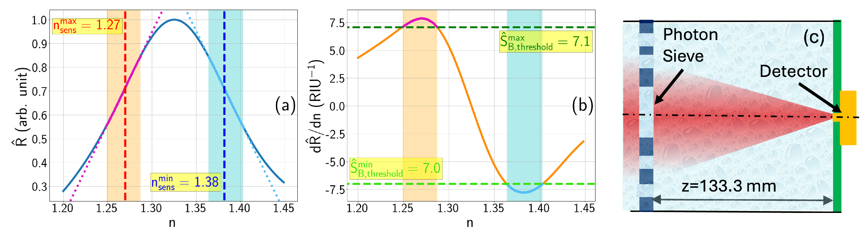
Refractometric Sensing

As previously discussed, the proposed masks and associated photon sieves are introduced here as optical elements capable of focusing light and generating signals related to the properties of a fluid traversing the photon sieve. Optically, one of the most significant parameters of the fluid is its index of refraction, n, and how it may vary due to physical or chemical changes. To determine this value, we have calculated the normalized sensitivity, ${\widehat{S}}_B$, and the Figure of Merit (FOM) of a refractometric sensor that relies on the variation of the irradiance distribution along the axis for one of the proposed masks. This normalized sensitivity can be defined as [36].

$${\widehat{S}}_B=\left|{\displaystyle \frac{\partial \widehat{R}}{\partial n}}\right|,$$

(9)

where $\widehat{R}$ is the dimensionless normalized responsivity of the optoelectronic detection system, which can be easily adapted to the particular mechanism of irradiance detection [37]. The modulus denotes that the decreasing or increasing change is not of importance. Using ${\widehat{S}}_B$, it is possible to define the FOM as [37]

$$\mathrm{F}\mathrm{O}\mathrm{M}={\displaystyle \frac{{\widehat{S}}_B}{\mathrm{\Delta }\widehat{R}}},$$

(10)

where $\mathrm{\Delta }\widehat{R}$ describes the applicable resolvable interval in responsivity. This optoelectronic interrogation method does not necessitate the use of spectrometers or goniometers, unlike sensors based on plasmonic resonances.

It is well known that the focal length of any diffractive element strongly depends on the index of refraction of the propagating medium. This dependence is described by the effective wavelength in Equation (1) as $\lambda ={\lambda }_0/n$, where ${\lambda }_0$ is the wavelength in vacuum, and n is the index of refraction of the medium (assuming homogeneity). Since the geometry of the mask cannot be modified, the effect of this change in refractive index is a corresponding change in the focal length of the photon sieve, as follows:

$$f^{\prime }\left(n\right)={\displaystyle \frac{n{r}_1^2}{{\lambda }_0}},$$

(11)

where $r_1$ is the radius of the central hole of the PS.

As seen before, the RbR PS demonstrates a balanced performance in terms of optical behavior and permeability, which is why we have focused our analysis on this case. Practically, we evaluated the irradiance captured by a light detector with a 50 μm diameter pinhole, positioned at the focal plane of the PS. Using "Diffractio," we obtained the integrated irradiance on the detector as a function of the index of refraction. This focal plane is selected for a reference index of refraction, $n=1.333$. Figure 8a illustrates the normalized signal, $\widehat{R}\left(n\right)$, for the RbR mask when the detector is located at $f^{\prime }(n=1.333)=133.3$ mm. The distance between the PS and the detector remains fixed while varying the index of refraction. As expected, the plot reaches a maximum value of 1 at $n=1.333$. For a refractometric sensor based on optoelectronic signals [37], we calculated the normalized sensitivity defined in Equation (9). This parameter is represented in Figure 8b, showing a local maximum of ${\widehat{S}}_{B,\max }=7.86$ RIU⁻¹ at $n_{\mathrm{sens}}^{\max }=1.27$ and a local minimum of ${\widehat{S}}_{B,\min }=7.77$ RIU⁻¹ at $n_{\mathrm{sens}}^{\min }=1.38$. These values of the index of refraction correspond to the largest changes in intensity. Around these values, we can define a dynamic range where the signal’s linearity is nearly preserved. Assuming a 10% variation in ${\widehat{S}}_B$ (see the horizontal dotted lines in Figure 8), we obtain the corresponding intervals in the index of refraction: $[1.249,1.287]$ marked in orange and $[1.364,1.403]$ marked in blue around the maximum and minimum locations, respectively. Moreover, assuming the signal can be resolved up to $\mathrm{\Delta }\widehat{R}={10}^{-3}$ from the maximum normalized value [38], the FOM of this system, defined in Equation (10), is ${\mathrm{F}\mathrm{O}\mathrm{M}}_{\max }=7860$ RIU⁻¹ and Nstea ${\mathrm{F}\mathrm{O}\mathrm{M}}_{\min }=7770$ RIU⁻¹, which are reasonable values for a refractometric sensor. The normalized sensitivity and FOM obtained for this design are highly competitive with those of plasmonic-based designs [38], including recent reports [39,40,41]. On the other hand, the center and interval of the dynamic range of refractometric sensors based on plasmonic resonances are fixed once the geometry is set. Practically, as shown in Figure 8c, the distance between the PS and the detector remains fixed, allowing the sensor to operate in two dynamic ranges (see colored bands in Figure 8) with similar sensitivities. These ranges are around two values of the index of refraction: $n_{\mathrm{sens}}^{\max }$ and $n_{\mathrm{sens}}^{\min }$, as shown in Figure 8a. These locations do not coincide with the maximum responsivity, Nstea $\widehat{R}$, which occurs at $n=1.333$ in the given example. For refractometric sensors based on plasmonic resonances, monitoring another medium requires changing the sensing element to shift the resonance to the wavelength with the highest sensitivity for the desired analyte refractive index. In our case, we can move to another interval in refractive index by simply adjusting the detector’s location, allowing the center of the dynamic range to be positioned almost at will. However, we acknowledge that refractometric sensors relying on intensity variations introduce practical constraints that should be considered before operation. Nonetheless, the simplicity and integrability of the proposed design offer significant advantages that may offset some practical drawbacks.

4. Conclusions

In this study, we implemented several photon sieve masks on an optical bench to evaluate their optical performance. Most masks utilized a merit function to maximize light at the focal region. We compared three mask generation methods: the Hole-by-Hole method, which iteratively generates holes using a merit function considering both irradiance and permeability; Nstea the Ring-by-Ring method, which fills one ring of equal circular holes at a time, maximizing irradiance (and permeability if necessary) at each step; Nstea and the Hole-in-Ring method, which opens circular holes within the contributive Fresnel zones, with diameters equal to the width of the given zone. All masks were designed with circular holes compatible with typical fabrication constraints and compared with the classical binary amplitude Fresnel zone plate (the Soret lens).

Photon sieves were implemented using a spatial light modulator in pure-amplitude mode. The focal region was scanned, and irradiance distributions were recorded for analysis. This approach allows for feasible experimental analysis of the masks’ optical performance before fabrication, providing an affordable benchmark to select the best-performing photon sieve for a given application. Using this experimental approach, we conducted a comparative analysis of various diffractive permeable lens designs to evaluate their behavior around the focal region. The study aimed to assess the efficiency of different designs in controlling and shaping light while maintaining permeability, crucial for optical applications involving the monitoring of running fluids.

We evaluated the depth of focus to determine the range over which the lens maintains sufficient irradiance, and measured transverse widths at the beam waist to assess the sharpness and lateral extent of the focal spot. Permeability was also considered fundamental, ensuring the lens design allows the transmission of both light and fluids without significant losses. These factors collectively help identify the most effective photon sieve configuration for practical applications. Beyond these fundamental parameters, the study investigated additional factors influencing beam quality and the experimental setup. The $M^2$ factor, a widely used metric in laser optics, was included to quantify the beam’s deviation from an ideal Gaussian distribution, directly affecting the efficiency of optical systems for collimation and focusing. Furthermore, generalized ellipticity was defined and examined to understand how unwanted distortions could arise and influence lens performance. One of the most significant aspects introduced in this study was the analysis of lens permeability, a key factor in ensuring the proper functionality of permeable diffractive lenses in applications where both light and matter must pass through the optical element, such as biomedical imaging, laser processing, and advanced optical systems involving running fluids. Among the designs evaluated, the RbR lens demonstrated a reasonable balance between focus quality and permeability, making it the most suitable option for future projects.

As a practical example, the capabilities of photon sieves as refractometric sensors for running fluids were computationally evaluated for the Ring-by-Ring mask with a focal length of Nstea $f^{\prime }=133.3$ mm. The evaluation of the Figure of Merit for this type of sensor reached a value of approximately 7860 RIU⁻¹. This approach also revealed two equivalent dynamic ranges that can be easily centered at the desired index of refraction.

In summary, by considering both ideal performance metrics and practical challenges, this study provided a comprehensive evaluation that highlights the strengths of different lens designs and addresses potential limitations in real-world applications. This validation enables the comparison of different designs before investing time and resources in fabricating non-optimal devices for a given application.

References

1. Khonina, S.N.; Kazanskiy, N.L.; Skidanov, R.V.; Butt, M.A. Advancements and Applications of Diffractive Optical Elements in Contemporary Optics: A Comprehensive Overview. Adv. Mater. Technol. 2024, 10, 2401028. [Google Scholar] [CrossRef]
2. Kim, H.J.; Aguillard, J.; Julian, M.; Bartram, S.; Macdonnell, D. Photon Sieve Design and Fabrication for Imaging Characteristics Using UAV Flight; NASA/TM; 2019-220252; National Aeronautics and Space Administration, Langley Research Center: Hampton, VA, USA, 2019.
3. Sabatyan, A.; Mirzaie, S. Efficiency-enhanced photon sieve using Gaussian/overlapping distribution of pinholes. Appl. Opt. 2011, 50, 1517–1522. [Google Scholar] [CrossRef]
4. Sabatyan, A.; Hoseini, S.A. Diffractive performance of a photon-sieve-based axilens. Appl. Opt. 2014, 53, 7331–7336. [Google Scholar] [CrossRef]
5. Davis, A.; Kühnlenz, F. Optical Design using Fresnel Lenses. Opt. Photonik 2007, 2, 52–55. [Google Scholar] [CrossRef]
6. Vila-Comamala, J.; Borrisé, X.; Pérez-Murano, F.; Campos, J.; Ferrer, S. Nanofabrication of Fresnel zone plate lenses for X-ray optics. Microelectron. Eng. 2006, 83, 1355–1359. [Google Scholar] [CrossRef]
7. Michette, A.G. Diffractive Optics II Zone Plates; Springer US: Greer, SC, USA, 1986; pp. 165–215. [Google Scholar] [CrossRef]
8. Baez, A.V. Fresnel Zone Plate for Optical Image Formation Using Extreme Ultraviolet and Soft X Radiation. J. Opt. Soc. Am. 1961, 51, 405–412. [Google Scholar] [CrossRef]
9. Soria-Garcia, A.; del Hoyo, J.; Sanchez-Brea, L.M.; Pastor-Villarrubia, V.; Gonzalez-Fernandez, V.; Elshorbagy, M.H.; Alda, J. Vector diffractive optical element as a full-Stokes analyzer. Opt. Laser Technol. 2023, 163, 109400. [Google Scholar] [CrossRef]
10. Yamada, K.; Watanabe, W.; Li, Y.; Itoh, K.; Nishii, J. Multilevel phase-type diffractive lenses in silica glass induced by filamentationof femtosecond laser pulses. Opt. Lett. 2004, 29, 1846–1848. [Google Scholar] [CrossRef]
11. Moreno, V.; Román, J.F.; Salgueiro, J.R. High efficiency diffractive lenses: Deduction of kinoform profile. Am. J. Phys. 1997, 65, 556–562. [Google Scholar] [CrossRef]
12. Andersen, G. Membrane photon sieve telescopes. Appl. Opt. 2010, 49, 6391–6394. [Google Scholar] [CrossRef]
13. Andersen, G.; Tullson, D. Photon sieve telescope. In Proceedings of the Space Telescopes and Instrumentation I: Optical, Infrared, and Millimeter, Orlando, FL, USA, 24–31 May 2006; Mather, J.C., MacEwen, H.A., de Graauw, M.W.M., Eds.; International Society for Optics and Photonics, SPIE: Bellingham, WA, USA, 2006; Volume 6265, p. 626523. [Google Scholar] [CrossRef]
14. Lambrou, T.P.; Anastasiou, C.C.; Panayiotou, C.G.; Polycarpou, M.M. A low-cost sensor network for real-time monitoring and contamination detection in drinking water distribution systems. IEEE Sens. J. 2014, 14, 2765–2772. [Google Scholar] [CrossRef]
15. Bernasconi, G.; Del Giudice, S.; Giunta, G.; Dionigi, F. Advanced pipeline vibroacoustic monitoring. In Proceedings of the Pressure Vessels and Piping Conference, Paris, France, 14–18 July 2013; American Society of Mechanical Engineers: New York City, NY, USA, 2013; Volume 55690, p. V005T10A008. [Google Scholar]
16. Oktem, F.S.; Kamalabadi, F.; Davila, J.M. High-resolution computational spectral imaging with photon sieves. In Proceedings of the 2014 IEEE International Conference on Image Processing (ICIP), Paris, France, 27–30 October 2014; pp. 5122–5126. [Google Scholar] [CrossRef]
17. Cao, Q.; Jahns, J. Focusing analysis of the pinhole photon sieve: Individual far-field model. J. Opt. Soc. Am. A 2002, 19, 2387–2393. [Google Scholar] [CrossRef]
18. Snigirev, A.; Kohn, V.; Snigireva, I.; Lengeler, B. A compound refractive lens for focusing high-energy X-rays. Nature 1996, 384, 49–51. [Google Scholar] [CrossRef]
19. Machado, F.; Zagrajek, P.; Monsoriu, J.A.; Furlan, W.D. Terahertz Sieves. IEEE Trans. Terahertz Sci. Technol. 2018, 8, 140–143. [Google Scholar] [CrossRef]
20. Cheng, C.; Cao, Q.; Bai, L.; Li, C.; Zhu, J.; Chen, W.; Mao, Y. High-efficiency square-hole single-mode waveguide photon sieves for THz waves. Appl. Opt. 2023, 62, 2403–2409. [Google Scholar] [CrossRef]
21. Rijfkogel, L.S.; Ghanbarian, B.; Hu, Q.; Liu, H.H. Clarifying pore diameter, pore width, and their relationship through pressure measurements: A critical study. Mar. Pet. Geol. 2019, 107, 142–148. [Google Scholar] [CrossRef]
22. Sanchez-Brea, L.M.; Soria-Garcia, A.; Andres-Porras, J.; Pastor-Villarrubia, V.; Elshorbagy, M.H.; del Hoyo Muñoz, J.; Torcal-Milla, F.J.; Alda, J. Diffractio: An open-source library for diffraction and interference calculations. In Proceedings of the Optics and Photonics for Advanced Dimensional Metrology III, Strasbourg, France, 7–11 April 2024; de Groot, P.J., Guzman, F., Picart, P., Eds.; International Society for Optics and Photonics, SPIE: Bellingham, WA, USA, 2024; Volume 12997, p. 129971B. [Google Scholar] [CrossRef]
23. Soria-Garcia, A.; Sanchez-Brea, L.M.; del Hoyo, J.; Torcal-Milla, F.J.; Gomez-Pedrero, J.A. Fourier series diffractive lens with extended depth of focus. Opt. Laser Technol. 2023, 164, 109491. [Google Scholar] [CrossRef]
24. Garcia-Lozano, G.; Mercant, G.; Fernandez-Rodriguez, M.; Torquemada, M.C.; Gonzalez, L.M.; Belenguer, T.; Cuadrado, A.; Sanchez-Brea, L.M.; Alda, J.; Elshorbagy, M. Experimental Analysis of the Spectral Reflectivity of Metallic Blazed Diffraction Gratings in the THz Range for Space Instrumentation. IEEE Trans. Terahertz Sci. Technol. 2025, 15, 8–16. [Google Scholar] [CrossRef]
25. Kang, E.K.; Lee, Y.W.; Ravindran, S.; Lee, J.K.; Choi, H.J.; Ju, G.W.; Min, J.W.; Song, Y.M.; Sohn, I.B.; Lee, Y.T. 4 channel × 10 Gb/s bidirectional optical subassembly using silicon optical bench with precise passive optical alignment. Opt. Express 2016, 24, 10777–10785. [Google Scholar] [CrossRef]
26. Chen, S.T.; Luo, T.S. Fabrication of micro-hole arrays using precision filled wax metal deposition. J. Mater. Process. Technol. 2010, 210, 504–509. [Google Scholar] [CrossRef]
27. Chen, S.; Zhang, L.; Zhao, Y.; Ke, M.; Li, B.; Chen, L.; Cai, S. A perforated microhole-based microfluidic device for improving sprouting angiogenesis in vitro. Biomicrofluidics 2017, 11, 054111. [Google Scholar] [CrossRef]
28. Jia, P.; Zhou, S.; Cai, X.; Guo, Q.; Niu, H.; Ning, W.; Sun, Y.; Zhang, D. High-fidelity synthesis of microhole templates with low-surface-energy-enabled self-releasing photolithography. RSC Adv. 2024, 14, 12125–12130. [Google Scholar] [CrossRef]
29. Pastor-Villarrubia, V.; Soria-Garcia, A.; Andres-Porras, J.; del Hoyo, J.; Elshorbagy, M.H.; Sanchez-Brea, L.M.; Alda, J. Optimum design of permeable diffractive lenses based on photon sieves. Optik 2024, 330, 172342. [Google Scholar] [CrossRef]
30. Pastor-Villarrubia, V.; Soria-Garcia, A.; del Hoyo, J.; Sanchez-Brea, L.M.; Alda, J. Permeable diffractive optical elements for real-time sensing of running fluids. In Proceedings of the Optical Sensors, Prague, Czech Republic, 24–26 April 2023; SPIE: Bellingham, WA, USA, 2023; Volume 12572, pp. 170–177. [Google Scholar]
31. Joignant, A.N.; Xi, Y.; Muddiman, D.C. Impact of wavelength and spot size on laser depth of focus: Considerations for mass spectrometry imaging of non-flat samples. J. Mass Spectrom. 2023, 58, e4914. [Google Scholar] [CrossRef]
32. Siegman, A.E. Defining, measuring, and optimizing laser beam quality. In Proceedings of the Laser Resonators and Coherent Optics: Modeling, Technology, and Applications, Los Angeles, CA, USA, 18–20 January 1993; Bhowmik, A., Ed.; International Society for Optics and Photonics, SPIE: Bellingham, WA, USA, 1993; Volume 1868, pp. 2–12. [Google Scholar] [CrossRef]
33. Rabiner, L.; Schafer, R.; Rader, C. The chirp z-transform algorithm. IEEE Trans. Audio Electroacoust. 1969, 17, 86–92. [Google Scholar] [CrossRef]
34. Bluestein, L. A linear filtering approach to the computation of discrete Fourier transform. IEEE Trans. Audio Electroacoust. 1970, 18, 451–455. [Google Scholar] [CrossRef]
35. Hu, Y.; Wang, Z.; Wang, X.; Ji, S.; Zhang, C.; Li, J.; Zhu, W.; Wu, D.; Chu, J. Efficient full-path optical calculation of scalar and vector diffraction using the Bluestein method. Light. Sci. Appl. 2020, 9, 119. [Google Scholar] [CrossRef]
36. Huang, D.W.; Ma, Y.F.; Sung, M.J.; Huang, C.P. Approach the angular sensitivity limit in surface plasmon resonance sensors with low index prism and large resonant angle. Opt. Eng. 2010, 49, 054403. [Google Scholar] [CrossRef]
37. Elshorbagy, M.H.; Cuadrado, A.; Romero, B.; Alda, J. Enabling selective absorption in perovskite solar cells for refractometric sensing of gases. Sci. Rep. 2020, 10, 7761. [Google Scholar] [CrossRef]
38. Elshorbagy, M.H.; Esteban, O.; Cuadrado, A.; Alda, J. Optoelectronic refractometric sensing device for gases based on dielectric bow-ties and amorphous silicon solar cells. Sci. Rep. 2022, 12, 18355. [Google Scholar] [CrossRef]
39. Khodaie, A.; Heidarzadeh, H.; Harzand, F.V. Development of an advanced multimode refractive index plasmonic optical sensor utilizing split ring resonators for brain cancer cell detection. Sci. Rep. 2025, 15, 433. [Google Scholar] [CrossRef] [PubMed]
40. Bouandas, H.; Kumar, R.; Benhaliliba, M.; Singh, S.; Garia, L. Plasmonic sensor design: Cu-SiO2-Ni-black phosphorus for enhanced surface plasmon resonance in visible regime. Microchim. Acta 2025, 192, 114. [Google Scholar] [CrossRef] [PubMed]
41. Bouandas, H.; Slimani, Y.; Daher, M.G.; Djemli, A.; Fatm, M.; Aldossari, S.A.; Mika, S. Design of an Advanced Sensor Based on Surface Plasmon Resonance with Ultra-High Sensitivity. Plasmonics 2025. [Google Scholar] [CrossRef]
Figure 1. Permeable lenses for study. (a) HbH WMF with w = 1.0, (b) HbH WMF with w = 0.7, (c) HbH GMF, (d) RbR, (e) HiR and (f) FZP. This last mask is taken as the reference for our analysis.
Photonics 12 00486 g001
Figure 2. Experimental setup. The light source is a He-Ne laser, which, after being spatially filtered and expanded, passes through a linear polarizer (P0) and a quarter waveplate (Q0) to achieve a circular polarization state before entering the system. The beam fully illuminates the aperture of the SLM under normal incidence conditions. To operate the SLM in amplitude mode, the polarization elements in both the PSG and PSA are correctly oriented. Each subsystem, PSG and PSA, is equipped with a polarizer (P1 and P2) and a quarter waveplate (Q1 and Q2), respectively. After passing through the PSG, the beam is redirected by a flat mirror to compact the setup. A beam splitter is inserted to ensure normal incidence on the SLM plane. The SLM plane is imaged onto another plane via the 4 f system, which is configured to provide a lateral magnification of −1. Subsequently, the focal region of the PS mask is scanned by moving the camera on a controllable linear stage.
Photonics 12 00486 g002
Figure 3. Maps of the images captured at z = 89 mm (a), z = 100 mm (b), and z = 107 mm (c) for the RbR mask. (d) Evolution of the generalized ellipticity, η ^ , with z. This plot crosses η ^ = 0 at z 99.4 mm, which almost coincides with the nominal focal length of the lens f = 100 mm. The stars in the ellipticity curve denote the locations of the transversal irradiance distributions presented in (a), (b), and (c) in violet, blue, and green colors, respectively.
Photonics 12 00486 g003
Figure 4. The depth of field (DOF) is determined using the FWHM criteria. For the RbR case, the numerical value is D O F = 8.7 mm. To obtain a more precise DOF value, we linearly interpolated the experimental data. The FWHM is set at 0.6, as the minimum value of this evolution, occurring at 0.2, has been considered.
Photonics 12 00486 g004
Figure 5. 2D Gaussian fit for the RbR mask at z = 89.4 mm. (a) Original irradiance, (b) preprocessed irradiance, and (c) Gaussian fit. The plots in (d) and (e) represent the profiles along the X and Y axes, respectively, rotated by an angle α = 34 . 1 . The dotted red lines represent the original profile obtained from (a); the dotted green lines show the preprocessed profile as depicted in (b); and the solid black lines are the Gaussian fit profiles corresponding to the map in (c).
Photonics 12 00486 g005
Figure 6. Gaussian propagation fitting for the RbR mask. These fits calculate the beam waist size ( ω 0 ), divergence ( θ 0 ), and M 2 factor for each axis. The blue fit considers only the values of ω ( z ) around the waist (red dots). The direction X , ω x , is shown in (a), and ω y in (b). These curves exhibit a larger θ 0 value compared to the green curve, which represents the Gaussian evolution fitted with all measured points (orange dots).
Photonics 12 00486 g006
Figure 7. Experimental data. X Z and Y Z views of the beam for the HbHWMF with w = 1.0 (a,b), HbHWMF with w = 0.7 (c,d), HbHGMF (e,f), RbR (g,h), HiR (i,j) and FZP (k,l) photon sieves. The representation uses a normalized logarithmic scale in the range [0,1], consistent across all masks. The scale bars differ for the axial, Z, and transverse directions, X and Y, but are applicable to all plots.
Photonics 12 00486 g007
Figure 8. (a) Normalized responsivity, R ^ ( n ) , for the integrated signal of a detector with a diameter of 50 μm, located at z = f ( n = 1.333 ) = 133.3 mm. (b) Variation of the normalized responsivity with respect to the index of refraction, Nstea R ^ / n . The magnitude of this derivative can be considered to be the normalized sensitivity, S ^ B , for the normalized responsivity, R ^ ( n ) , as defined in Equation (9). This calculation is performed for the RbR mask. The colored bands around the value of n represent the dynamic range, considering that S ^ B exceeds 0.9 of its maximum value. The presence of two dynamic ranges indicates the sensor’s capability to explore two different regions with the same configuration. (c) Optical setup where a collimated beam, after passing through the photon sieve, focuses the light on a detector located at a distance of z = 133.3 mm, which remains fixed while varying n.
Photonics 12 00486 g008