Ultrafast Laser Beam Profile Characterization in the Front-End of the ELI-NP Laser System Using Image Features and Machine Learning

Abstract

Ultrafast laser systems, implemented at the ELI-NP, require exceptional beam quality and spatial stability due to their femtosecond pulse durations and extremely high peak powers. This work presents a diagnostic and computational framework for analyzing the ELI-NP Front-End beam characteristics, where spatial coherence and precise pulse shaping are essential for reliable amplification and experimental consistency. The methodology integrates classical beam diagnostics with image processing and machine learning tools to evaluate anomalies based on high-resolution beam profile images. We use centroid tracking to monitor pointing fluctuations, statistical intensity analysis to detect energy instabilities, and Sobel-based edge detection to evaluate beam sharpness and extract structural features from the beam image. Geometric parameters such as ellipticity, roundness, and symmetry indicators are extracted and examined over time. The system applies an unsupervised Isolation Forest algorithm to detect subtle or short-lived anomalies, identifying irregularities without relying on predefined thresholds. These diagnostics are supported by visual plots and statistical summaries, offering a clear picture of the beam’s behavior under real operating conditions. Results confirm that this integrated approach effectively captures major and minor beam instabilities, making it a practical tool for continuous monitoring and performance optimization in ultrafast laser systems.

1. Introduction

Femtosecond laser systems have become a fundamental tool in ultrafast optics, supporting a wide array of high-precision applications, including micromachining [1], nonlinear spectroscopy [2], optical coherence tomography [3], and biomedical imaging [4,5]. These systems generate pulses as short as 10⁻¹⁵ s with extremely high peak powers [6], which makes them highly sensitive to minor disturbances. Optical misalignments, thermal drift, mechanical vibrations, and even subtle environmental changes can affect beam quality, causing shifts in centroid position, shape deformations, and fluctuations in intensity distribution [7]. Precise characterization and monitoring of laser beam quality are critical to the success of these applications. Instabilities in the beam profile or pointing can directly degrade the resolution of micromachining processes, limit the sensitivity of spectroscopic measurements, and impact the accuracy of imaging systems. Therefore, developing more sensitive, real-time beam diagnostic methods has become essential in ultrafast optics research.

While various beam diagnostic tools exist, most rely on isolated or threshold-based measurements such as centroid tracking, beam width estimation, or basic intensity histograms [8,9,10,11]. Standardized methods such as those outlined in [12] are often employed to characterize femtosecond laser beams, specifying parameters like beam width, divergence, M² factor, and beam propagation ratios. While these standards provide reliable frameworks for basic beam quality assessments, they often fall short in capturing dynamic, transient, or low-magnitude anomalies in rapidly evolving laser systems. These conventional methods are often limited in scope. They tend to miss short-lived or low-magnitude anomalies, struggle with complex beam dynamics, and are unsuitable for adaptive, automated analysis in changing experimental environments. As laser systems become more sophisticated and performance demands increase, these limitations become more apparent. Recent advances in machine learning provide powerful new tools for beam diagnostics, offering the ability to automatically detect complex, nonlinear anomalies that may elude traditional threshold-based methods. Machine learning algorithms, such as anomaly detection models, can learn the statistical characteristics of stable beam behavior and flag subtle deviations without requiring manual supervision or predefined error limits. This capability is particularly valuable in high-repetition-rate, high-power laser systems where manual monitoring becomes impractical.

The methodology proposed in this work is built around a unified framework that integrates five core diagnostic strategies: spatial tracking [13], intensity statistics [14], beam shape analysis [15], edge detection [16], and machine learning-based anomaly detection [17]. Beam centroid coordinates are computed for each profile image to monitor pointing stability at a sub-pixel level. Simultaneously, we evaluate statistical metrics such as mean intensity and variance to capture fluctuations in energy distribution, which can reflect gain instabilities or optical disturbances. Sobel gradient-based edge detection is used to assess beam sharpness and structural clarity. The approach also includes geometric shape analysis, where beam ellipticity and roundness are extracted to evaluate the symmetry and focus of the beam over time. Advanced optical diagnostics, such as multispectral fringe projection profilometry, have also demonstrated potential in capturing high-resolution beam deformation patterns in a single shot [18]. We apply an unsupervised Isolation Forest machine learning technique to detect frames that deviate from typical behavior [19]. These anomalies often correspond to real physical changes, sudden lensing effects, thermal shifts, slight mirror movement, or even air turbulence in the lab [20,21]. By catching these subtle patterns early, the system provides practical insights that are easy to miss through manual inspection.

By combining mathematical precision, data processing, and intelligent pattern recognition, this work establishes a new standard for ultrafast laser beam diagnostics to meet the high-performance demands of facilities like the ELI-NP Front-End, where precision, reliability, and predictive maintenance are essential for success in high-intensity laser experiments. Beyond the current study, further work will integrate these diagnostic techniques into real-time feedback loops for dynamic beam correction and predictive maintenance of high-power laser systems.

2. Experimental Details and Image Acquisition

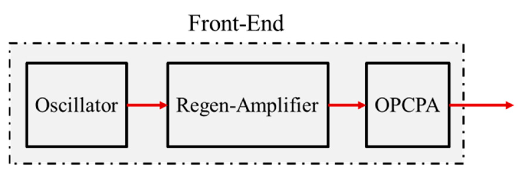
A simplified block diagram of the ELI-NP Front-End laser system is shown in Figure 1. It begins with a mode-locked oscillator that generates low-energy seed pulses amplified through a regenerative amplifier, and further pulses are amplified using an Optical Parametric Chirped Pulse Amplifier (OPCPA) [22,23,24] to preserve the broad spectral bandwidth necessary for femtosecond pulse durations. The result is a beam with pulse energies exceeding 10 mJ, pulse durations of about 20 picoseconds, and a spectral bandwidth greater than 63 nm (FWHM), operating at a repetition rate of 10 Hz.

The dataset analyzed in this study comprises 100 sequential profile images of a laser beam acquired from the Front-End of the ELI-NP high-power laser system [25,26]. The beam images are captured using a high-resolution CCD camera (ACA2440-20gm, Basler, Inc., Ahrensburg, Germany). The camera is operated in Mono 12-pixel format mode, providing 12-bit grayscale images to maintain high dynamic range and precise intensity mapping. Exposure times are optimized during the acquisition to avoid saturation, typically set between 30 and 100 microseconds, depending on the beam intensity after attenuation. The CCD camera is positioned at the diagnostic output of the Front-End laser chain, where beam quality is critically evaluated before further amplification stages. The laser beam is attenuated using a calibrated optical attenuation system composed of neutral-density filters to protect the camera sensor from high-intensity damage. The attenuation system is routinely checked to ensure that no ghost reflections or beam distortions affect the captured profiles, preserving the original beam structure as accurately as possible. The Front-End laser system is operated at a repetition rate of 10 Hz, delivering 10 pulses per second, while the image acquisition process is performed at a much slower sampling rate over an extended period. One hundred images are captured over approximately 4 h, resulting in an average acquisition interval of roughly 144 s (i.e., 2 min and 24 s) per image.

The slower sampling rate help us to build a long-term view of beam behavior over the extended operations instead of monitoring pulse-to-pulse variations. This method makes it possible to detect subtle drifts, thermal changes, vibrations, or alignment problems that are hard to notice when analyzing every single laser pulse. Environmental conditions are carefully controlled, with a clean room and room temperature maintained at 22 ± 1 °C and standard vibration isolation measures to minimize external disturbances. The imaging system is connected to a custom-built data acquisition and storage platform developed specifically for the ELI-NP facility. It enables real-time logging, frame indexing, and synchronized metadata recording. The complete dataset, including images and acquisition parameters, is stored in a dedicated database for reliable access, reproducibility, and laser system performance analysis. Each image is stored along with its timestamp and acquisition parameters, including CCD calibration and exposure settings, forming a structured dataset for analysis.

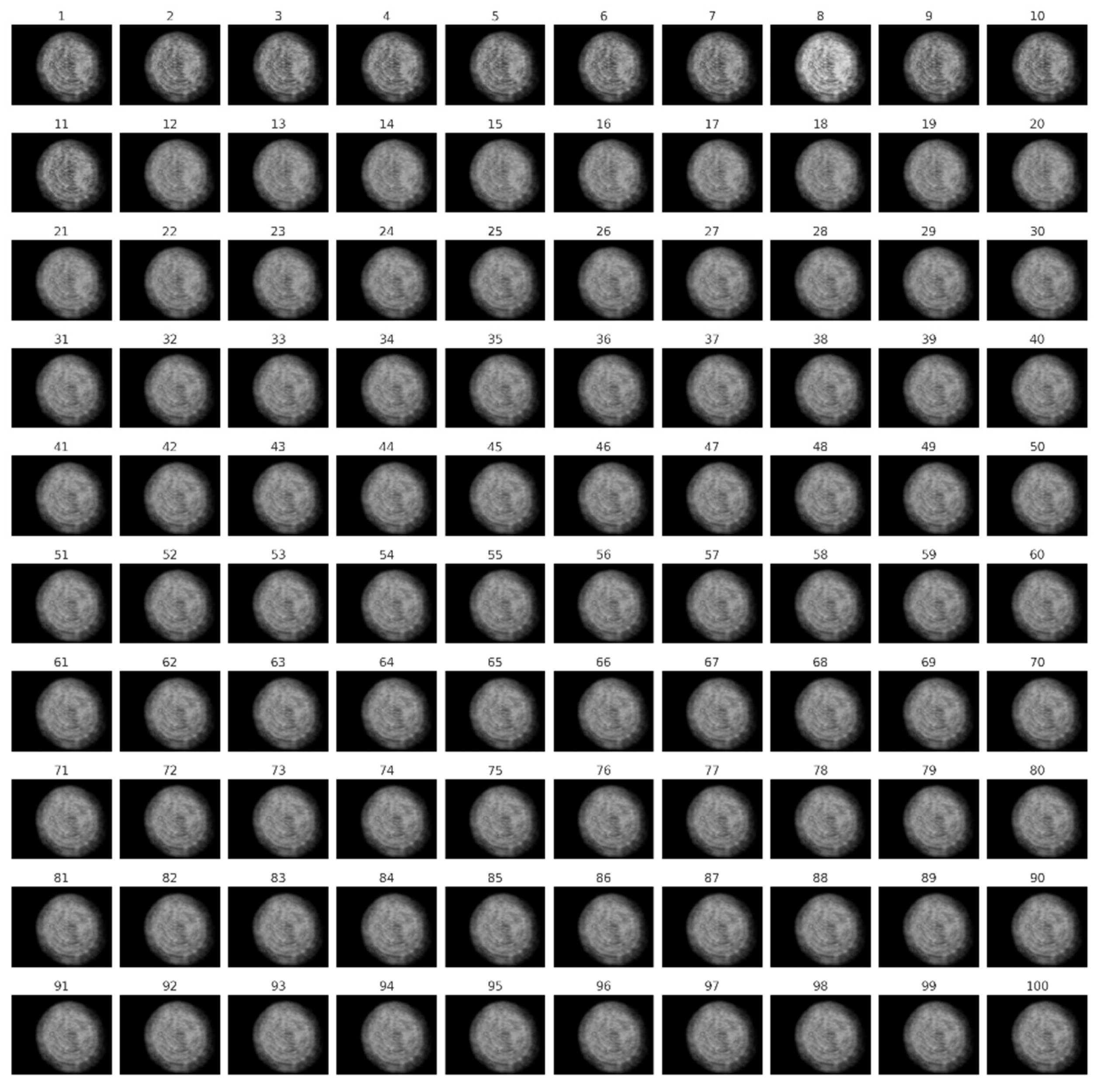
Figure 2 presents a composite overview of all 100 beam images, arranged sequentially from image 1 (top-left) to image 100 (bottom-right). Each image in the dataset shows the intensity pattern of the laser beam in two dimensions, recorded after the beam attenuation and normalization. When viewed as a composite, these images make it easy to spot how the beam’s shape and position change over time. For example, frames 8 and 10 clearly show differences in brightness, contrast, and edge sharpness, early signs that something unusual may have happened in the system. Later in the analysis, we confirm these visual clues using more detailed methods, including centroid tracking, intensity variance, Sobel edge detection, and machine learning through the Isolation Forest algorithm. This careful data collection and organized storage form a strong base for the more advanced analysis that follow.

3. Beam Profile Analysis, Results, and Visualization

3.1. Centroid Calculation

The centroid, the center point of the beam’s intensity distribution for each of the 100 recorded images, is calculated to evaluate how stable the beam is over time. The centroid coordinates (x_c, y_c) use a standard center-of-mass formula, as in Equations (1) and (2).

$$x_c={\displaystyle \frac{\sum _{i=1}^M\sum _{j=1}^N{x}_{ij}I\left(x_{ij}\right)}{\sum _{i=1}^M\sum _{j=1}^{N}I\left(x_{ij}\right)}}$$

(1)

$$y_c={\displaystyle \frac{\sum _{i=1}^M\sum _{j=1}^N{y}_{ij}I\left(y_{ij}\right)}{\sum _{i=1}^M\sum _{j=1}^{N}I\left(y_{ij}\right)}}$$

(2)

I(x,y) is the pixel’s intensity at coordinates (x,y), and M × N is the image resolution.

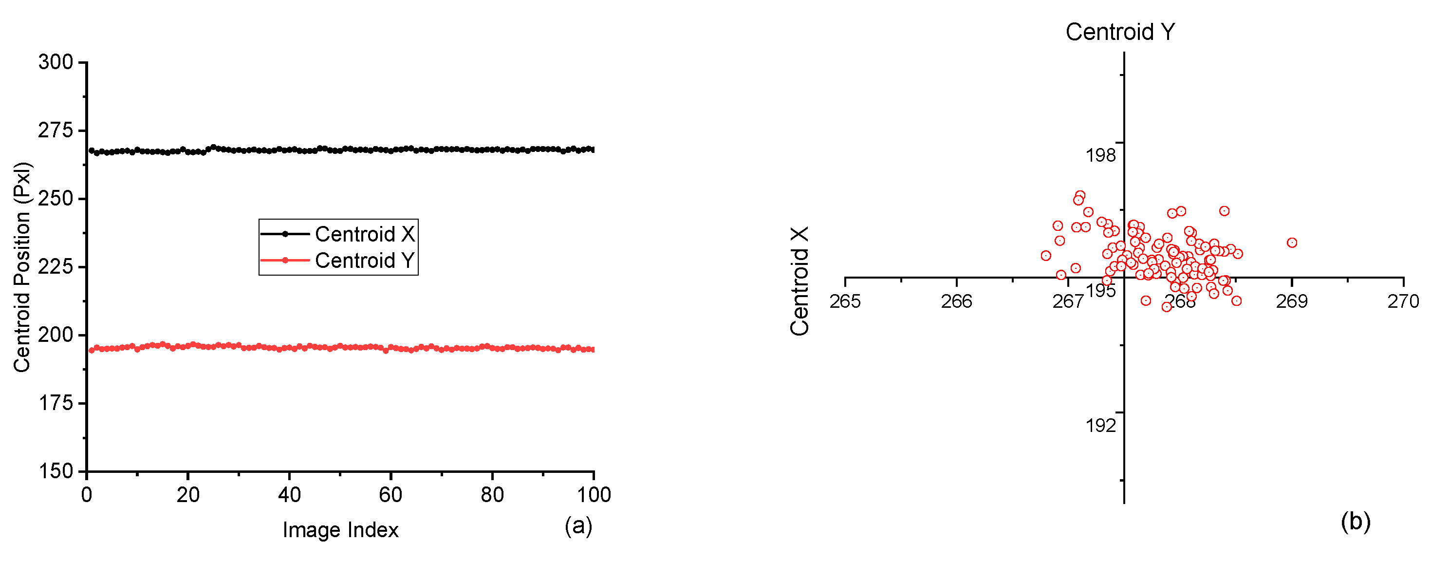
We tracked how these centroids moved across all images to assess pointing stability. Figure 3a shows a time-series plot of the centroid positions in the X and Y directions. The X-axis represents the image index, ranging from 0 to 100, and the Y-axis indicates the centroid position in pixel units. The X-centroid hovers at around 270 pixels, while the Y-centroid stays close to 195, with only small fluctuations, typically within ±2 pixels, which suggests that the laser beam is highly stable during operation.

Figure 3b presents a scatter plot of the centroids on the X–Y plane for better visualization and overall spatial jitter. The points form a dense, nearly circular cluster, showing no strong directional drift. This compact spread indicates that any movement is random and isotropic rather than systematic. This spatial representation is critical for identifying directional bias, potential elliptical jitter, or beam drift. Centroid analysis is essential in systems with critical tight beam alignment. Even small drifts can lead to misalignment in downstream optics. The fact that the beam stayed centered with minimal jitter shows the system was well aligned and stable throughout the data acquisition process.

3.2. Beam Intensity Statistics

The mean intensity and variance are calculated using Equations (3) and (4) for each image to check the beam’s brightness consistency.

$$\mu ={\displaystyle \frac{1}{MN}}{\sum }_{i=1}^M{\sum }_{j=1}^{N}I\left(x_{ij}\right)$$

(3)

$${\sigma }^2={\displaystyle \frac{1}{MN}}{\sum }_{i=1}^M{\sum }_{j=1}^N{\left(I\left(x_{ij}\right)-\mu \right)}^2$$

(4)

μ is the mean intensity, which shows the average brightness/intensity in each image, and σ² is the variance, which shows how much the intensity varies across the image. The square root of variance √σ² = σ is the standard deviation, representing the spread or non-uniformity in pixel intensity. M × N is the total number of pixels in each image (i.e., image resolution), and I(x_ij) is the pixel’s intensity (i,j).

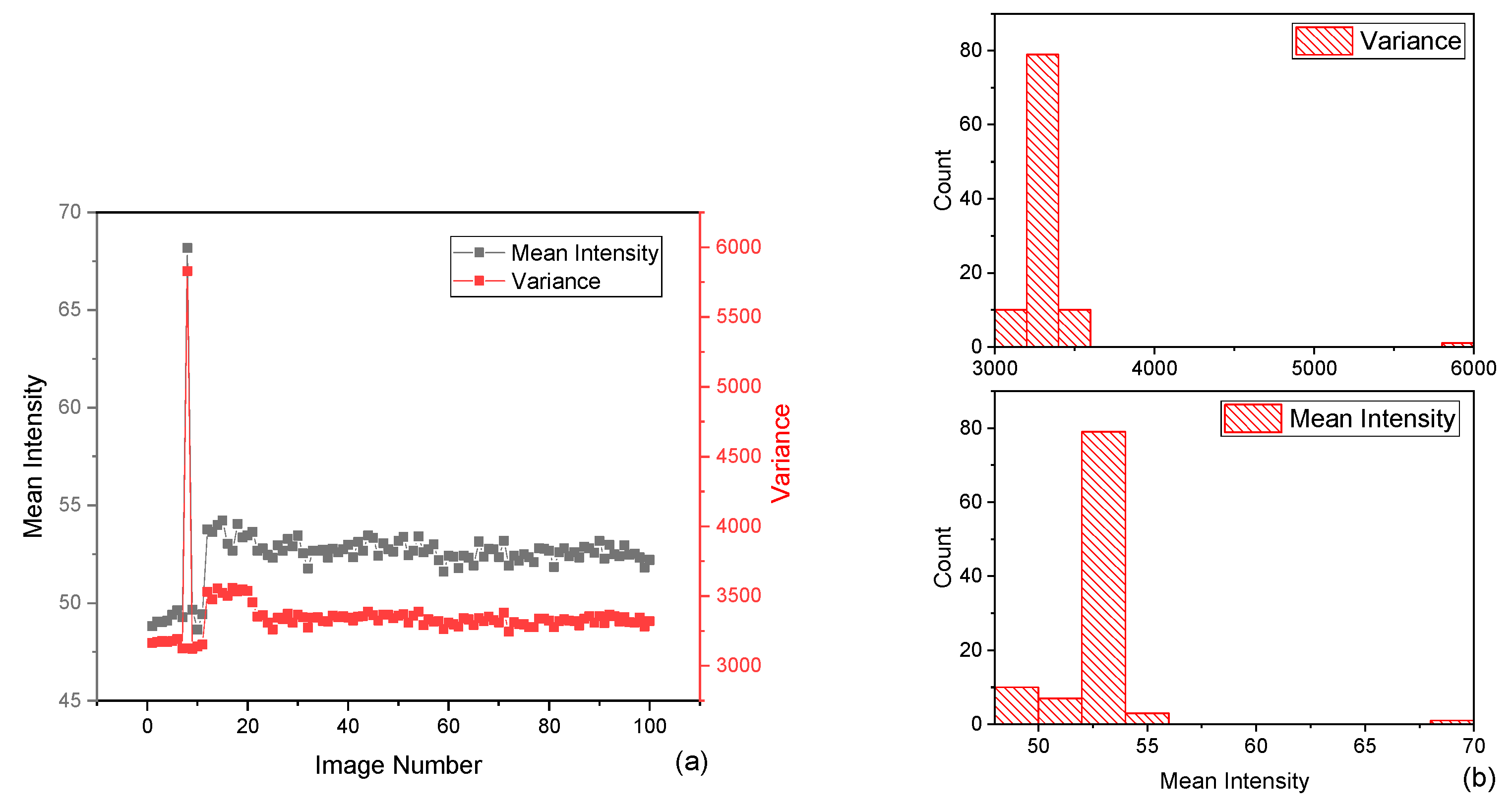
In Figure 4a, the X-axis represents the image number, the left Y-axis indicates the mean intensity in grayscale levels, and the right Y-axis shows the variance in the same units. Most mean intensity values lie in a stable range of around 50 to 53, with an initial spike below frame 10, where a few images briefly exceed 65. The variance follows the same trend; a large spike (around 6000) appears in the first few frames, then drops and stabilizes at around 3300. These early peaks may indicate transient optical artifacts such as reflections, calibration frames, or sudden energy fluctuations, and high initial variance signifies hot spots or non-uniform intensity patterns in the beam, which are absent in most subsequent frames.

The histograms in Figure 4b show two statistical features. The top panel displays the distribution of variance values, with most images clustered tightly around the 3300 mark and a few outliers reaching up to 6000, confirming the temporal anomaly in the line plot. The bottom panel presents the histogram of mean intensity, with most frames centered around 53 and only a small number showing significantly higher brightness. These statistical analyses are meaningful because they quantify beam quality and reveal inconsistencies that may not be visible through simple image inspection. Monitoring intensity and its variance provides essential insight into beam quality. A low variance paired with a stable mean suggests uniform energy delivery, critical for applications involving precision focusing or energy-sensitive interactions. These metrics also serve as early indicators of gain fluctuation, alignment drift, or contamination in the optical path.

3.3. Edge Detection

A classical Sobel gradient operator is employed across 100 sequential beam images to evaluate spatial sharpness and edge definition in the laser beam profiles. Before applying edge detection, a 2D Gaussian filter [27] is used to suppress high-frequency noise and prevent false edge detection. The Gaussian function is defined in Equation (5).

$$G\left(x,y\right)={\displaystyle \frac{1}{2\pi {\sigma }^2}}exp\left(-{\displaystyle \frac{x^2+y^2}{2{\sigma }^2}}\right)$$

(5)

The variable σ controls how much the image is blurred, and a larger σ means more smoothing (x,y), representing the pixel’s position relative to the center of the blur. This filtering helps reduce random noise while preserving the main structure of the beam.

After smoothing, the Sobel gradient/operator [28,29] is applied to detect intensity changes in the horizontal and vertical directions. The gradient components are defined by Equation (6). G_x and G_y show how brightness changes across the image, and the overall edge strength at each pixel is given by Equation (7).

$$G_x={\displaystyle \frac{\partial I}{\partial x}}, G_y={\displaystyle \frac{\partial I}{\partial y}}$$

(6)

$$G\left(x,y\right)=\sqrt{{G_x^2+G}_y^2}$$

(7)

Then, the average gradient value for the image is calculated with Equation (8).

$$\overline{G}={\displaystyle \frac{1}{MN}}{\sum }_{x=1}^M{\sum }_{y=1}^{N}G\left(x,y\right)$$

(8)

Figure 5a shows the average Sobel gradient Ḡ for each of the 100 images. The X-axis represents the image number, and the Y-axis shows the average edge sharpness. Some frames stand out with higher or lower values. For example, image 10 has a high gradient of about 28, meaning the beam is well focused, with sharp edges. In contrast, image 91 has a much lower value, of around 18, which suggests the beam is more blurred or out of focus. The peak near image 10 may have been caused by a brief change in the optical setup, a small alignment shift, or an interference pattern that made the beam appear sharper. Figure 5b shows 10 sample beam images from across the dataset to better understand this. Each image is labeled with its gradient value. The visual patterns match the data: images with higher gradient values, like image 10, have clear, sharp edges, while those with lower values, like image 90, appear soft and less defined. This gradient analysis is a useful way to measure how focused the beam is over time and detect any sudden sharpness changes that could affect system performance.

3.4. Beam Shape Metrics

Beam symmetry is analyzed using ellipticity and roundness, which describe the overall shape and balance of the beam profile in each image. Ellipticity is calculated as the ratio of the beam width in the X-direction (w_x) to the width in the Y-direction (w_y), as in Equation (9).

$$E={\displaystyle \frac{w_x}{w_y}}$$

(9)

Roundness is the ratio of the smaller beam width to the larger one, regardless of direction, as in Equation (10).

$$R={\displaystyle \frac{w_{min}}{w_{max}}}$$

(10)

The beam widths w_x and w_y used in these calculations are derived from fitting a Gaussian function to the beam’s intensity distribution in each direction or determining the full width at half maximum (FWHM).

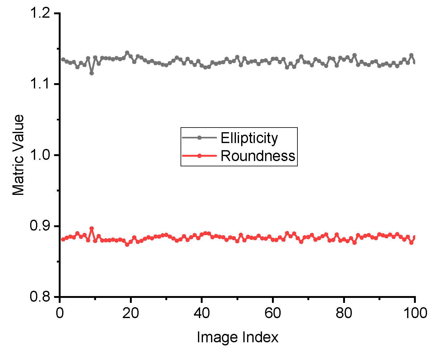
Ellipticity and roundness would be close to 1 in a perfectly circular beam. Figure 6 illustrates the temporal behavior of two beam shape metrics, ellipticity and roundness, across 100 sequential images. The image index ranges from 0 to 100 on the horizontal axis, while the vertical axis indicates the metric values for ellipticity and roundness. The ellipticity remains around 1.13 throughout the dataset, meaning the beam is slightly stretched in one direction—about 13% wider horizontally than vertically. The roundness stays near 0.89, confirming that the beam keeps an elliptical shape with only minor variations. These results indicate that the beam shape is stable over time. The slight asymmetry is consistent and does not show any abrupt changes, which suggests good optical alignment and no significant deformation during the measurement period. Shape metrics like these are especially important in high-power and ultrafast laser systems, where even small distortions can affect beam focusing and energy delivery. Regular monitoring of ellipticity and roundness helps detect early signs of misalignment, thermal effects, or other disturbances in the optical path.

3.5. Anomaly Detection Using Isolation Forest

After extracting various beam parameters from the dataset, we applied anomaly detection to identify frames that showed unusual behavior automatically. This step helps catch short-term instabilities or small deviations that might not be obvious in standard plots. We used the Isolation Forest algorithm, an unsupervised machine learning method, to detect outliers. It works by building a set of decision trees to isolate each data point. Points that are isolated quickly, meaning they behave very differently from the rest, are marked as anomalies. The anomaly score for each frame is calculated using Equation (11).

$$s\left(x,n\right)={\displaystyle \frac{2^{-E\left(h\left(x\right)\right)}}{c\left(n\right)}}$$

(11)

E(h(x)) is the average number of splits (path length) needed to isolate the data point x, and c(n) is a normalization factor based on the total number of points n; a lower path length means a higher anomaly score.

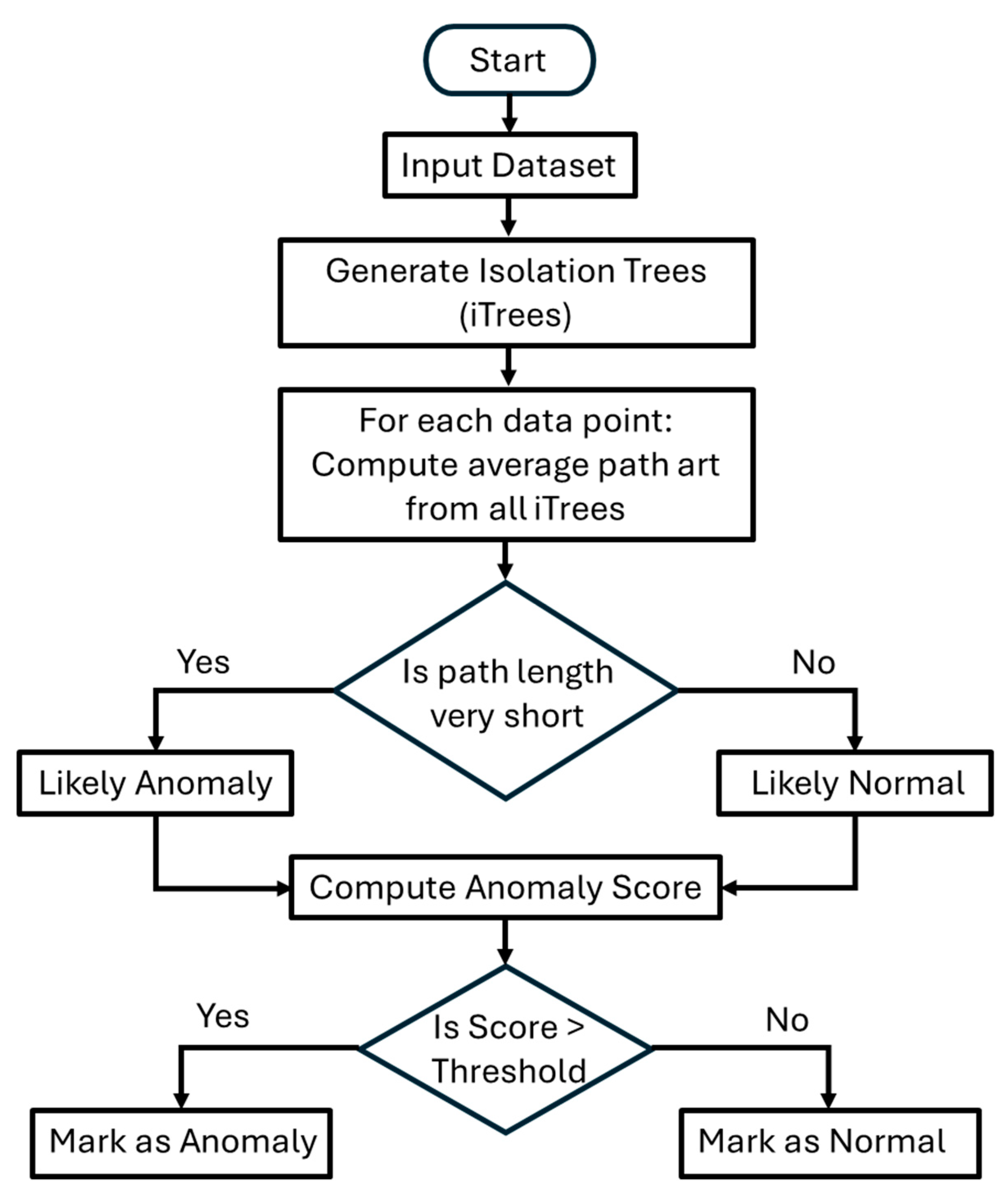
Figure 7 provides the flowchart diagram of the Isolation Forest process, which works by randomly selecting features and splitting values to construct decision trees and then computing the path length required to isolate each data point. Decision nodes assess whether the path length is short and the calculated anomaly score exceeds a defined threshold. Based on these conditions, the data point is classified as either an anomaly or normal.

We applied the Isolation Forest algorithm to four key beam features, i.e., ellipticity, roundness, mean intensity, and Sobel gradient. The goal was to identify frames with unusual values that may indicate temporary beam instability. The anomaly detection results are presented in Figure 8, with each sub-figure focusing on one parameter. Figure 8a shows anomalies based on beam shape; image frames 10, 20, 65, 83, and 99 are flagged due to small but noticeable changes in ellipticity and roundness. These shape deviations may have resulted from thermal lensing, alignment drift, or mechanical vibration, even if they are not obvious in the raw images. Figure 8b presents the detection results for mean intensity; image frame 10 shows a sharp spike in brightness, significantly higher than in the rest of the dataset, which may reflect a sudden energy fluctuation, an optical reflection, or a disturbance in the laser gain. Figure 8c highlights anomalies in Sobel gradient values, which indicate beam edge sharpness; again, image frame 10 is marked as an outlier, with a gradient of around 28, much higher than that of the surrounding frames, which may suggest a momentary increase in beam focus or clarity, possibly due to a quick alignment change or transient optical effect. The consistent detection of frame 10 across multiple features reinforces its significance as a transient anomaly.

The fact that image frame 10 is independently identified as an anomaly across all three parameters of shape, intensity, and sharpness strengthens its significance as a real and measurable event. Detecting such frames is valuable for diagnosing short-lived disturbances that may not appear in average trends but still impact beam quality. This approach makes monitoring beam behavior more precise and makes responding to performance issues before they affect critical applications possible. These plots highlight the necessity of integrating such analysis into laser system monitoring and control, ensuring high performance and robust quality assurance for essential laser applications.

4. Discussion and Conclusions

The analysis presented in this work combines several image-based methods to evaluate the stability and quality of an ultrafast laser beam over time. By measuring centroid position, intensity fluctuations, edge sharpness, and beam shape, the system provides a complete picture of how the beam behaves under real operating conditions.

Each parameter offers specific insight. Centroid tracking confirmed that the beam’s pointing was stable, with minimal jitter across 100 frames. Intensity analysis showed that the beam maintained a consistent brightness level after a brief initial fluctuation. Sobel edge detection helped identify changes in focus or beam clarity, and shape metrics such as ellipticity and roundness demonstrated that the beam maintained a steady elliptical profile throughout the acquisition period. The use of Isolation Forest added an important layer of automated intelligence. It successfully identified short-term anomalies aligned with visible and statistical changes in beam features. Notably, frame 10 was flagged by multiple indicators, confirming it as a brief but significant disturbance. These types of events, though small, can affect downstream experiments, especially in high-precision setups where beam consistency is critical. This approach is effective because it combines standard measurements with automated detection. While traditional standards such as ISO 11146 offer well-established static beam quality characterization procedures, the proposed method extends beyond static measurements by enabling real-time dynamic monitoring and early anomaly detection.

Instead of relying on a single parameter or fixed threshold, the system monitors multiple features and adapts to the data. This makes it more sensitive to subtle instabilities and better suited for long-term diagnostics. While the current approach effectively identifies beam anomalies through image features and unsupervised learning, incorporating formal statistical hypothesis testing, such as the Chi-square test, could further strengthen outlier validation. Due to the relatively small dataset and the exploratory nature of this study, we focused on direct feature analysis and machine learning techniques. Future work could expand on this foundation by integrating statistical testing methods to enhance the robustness and generalizability of anomaly detection.

The proposed framework offers a practical and reliable method for beam monitoring in ultrafast laser systems. It captures overall trends and detects brief disturbances that might otherwise go unnoticed. The approach is flexible, scalable, and well suited for integration into routine laser system maintenance, alignment checks, or performance optimization. Although the current implementation is based on offline analysis, the Isolation Forest algorithm processes each beam frame in under 3 milliseconds on standard desktop hardware. This demonstrates that the machine learning approach is computationally efficient and can handle large datasets rapidly. While no direct speed benchmark was conducted against traditional statistical methods, all implemented techniques proved lightweight and effective, including image feature extraction and machine learning-based anomaly detection. We selected Isolation Forest parameters that promote generalization to address concerns about overfitting due to the limited number of beam profile images. Specifically, we used 100 trees with a subsample size of 64 per tree. These settings help reduce variance and improve robustness. Furthermore, since Isolation Forest is an unsupervised algorithm that relies on random subsampling and isolation principles rather than learned decision boundaries, it is inherently less prone to overfitting. This makes it particularly suitable for anomaly detection tasks in smaller, high-dimensional datasets such as ours. With further development, the framework could be adapted for real-time feedback and predictive control in advanced laser facilities.