Article

Mitigating the Impact of Satellite Vibrations on the Acquisition of Satellite Laser Links Through Optimized Scan Path and Parameters

1
Key Laboratory of Electronics and Information Technology for Space Systems, National Space Science Center, Chinese Academy of Sciences, Beijing 100190, China
2
University of Chinese Academy of Sciences, Beijing 100049, China
3
National Space Science Center, Chinese Academy of Sciences, Beijing 101499, China
4
State Key Laboratory of Space Weather, National Space Science Center, Chinese Academy of Sciences, Beijing 100190, China
*
Author to whom correspondence should be addressed.
Photonics 2025, 12(5), 444; https://doi.org/10.3390/photonics12050444
Submission received: 25 March 2025 / Revised: 27 April 2025 / Accepted: 29 April 2025 / Published: 4 May 2025

Abstract

:
In the past two decades, there has been a tremendous increase in demand for services requiring a high bandwidth, a low latency, and high data rates, such as broadband internet services, video streaming, cloud computing, IoT devices, and mobile data services (5G and beyond). Optical wireless communication (OWC) technology, which is also envisioned for next-generation satellite networks using laser links, offers a promising solution to meet these demands. Establishing a line-of-sight (LOS) link and initiating communication in laser links is a challenging task. This process is managed by the acquisition, pointing, and tracking (APT) system, which must deal with the narrow beam divergence and the presence of satellite platform vibrations. These factors increase acquisition time and decrease acquisition probability. This study presents a framework for evaluating the acquisition time of four different scanning methods: spiral, raster, square spiral, and hexagonal, using a probabilistic approach. A satellite platform vibration model is used, and an algorithm for estimating its power spectral density is applied. Maximum likelihood estimation is employed to estimate key parameters from satellite vibrations to optimize scan parameters, such as the overlap factor and beam divergence. The simulation results show that selecting the scan path, overlap factor, and beam divergence based on an accurate estimation of satellite vibrations can prevent multiple scans of the uncertainty region, improve target satellite detection, and increase acquisition probability, given that the satellite vibration amplitudes are within the constraints imposed by the scan parameters. This study contributes to improving the acquisition process, which can, in turn, enhance the pointing and tracking phases of the APT system in laser links.

1. Introduction

In the past two decades, there has been a significant increase in internet usage and the demand for services such as video conferencing, live streaming, high-speed broadband, 5G wireless networks and beyond, the Internet of Things (IoT), broadcasting services, and satellite communications [1,2,3]. This growth has led to a surge in the number of users and data requirements. Conventional RF technology, which is widely used for these services, has limited bandwidth, and the radio frequency spectrum has become congested due to its widespread use in wireless networks (e.g., 2G, 3G, 4G, Wi-Fi, satellite communications, and Bluetooth) [4,5,6]. As a result, RF-based systems are constrained in terms of data rates and their ability to support high-speed communication.
OWC technology can overcome the limitations of RF-based communication. Compared to current microwave communication systems [7,8], which provide data transmission rates of only hundreds of Mbps, OWC offers much higher communication rates ranging from 100 Mbps to 10 Gbps. Moreover, OWC provides superior anti-interception and interference capabilities, as well as excellent confidentiality, due to its small beam divergence and the point-to-point nature of optical/laser links [9,10]. Since OWC uses light (infrared, visible, and ultraviolet) rather than electromagnetic waves, it is largely immune to RF interference [11]. OWC, also known as free-space optical (FSO) communication, can be classified into uplink/downlink and inter-satellite laser links in satellite communication systems. These links are capable of meeting the demands of next-generation satellite networks, which require a high capacity and low latency [12,13,14,15]. Although OWC offers significant advantages, laser links are still subject to several disadvantages [4]. These include atmospheric conditions such as fog, snow, and rain, as well as atmospheric turbulence, which can cause beam wander, beam spread, scintillation, and divergence losses [16]. Other challenges include background noise, sky radiance, pointing (misalignment) losses, cloud blockage, atmospheric seeing, and fluctuations in the angle of arrival.
Similarly, inter-satellite laser links encounter different challenges. Although they are located far above the atmosphere and are not subjected to weather conditions or cloud outages, they face issues such as the Point Ahead Angle (PAA), Doppler shift due to relative motion, satellite platform vibrations, and background noise sources such as solar and celestial bodies [17,18].
In addition to these challenges, both uplink/downlink and inter-satellite laser links require precise pointing of the narrow beam to establish a LOS laser link. This process is managed by the APT system [19,20,21,22]. The focus of this study is on the acquisition phase, which is the first step in establishing communication. In this phase, an uncertainty area is scanned to locate the receiver satellite. Once the receiver detects the beacon light and acquisition is complete, the receiver redirects the laser beam to the transmitter to establish alignment (pointing) from both sides. This is followed by the tracking phase, which ensures that the laser signal remains locked.
The main tasks of the acquisition phase include the selection of acquisition schemes and the selection of scan paths [19,23,24]. Balancing the acquisition time and acquisition probability is a major challenge in the design of satellite communication systems using laser links and is the primary focus of this study. One of the critical factors affecting acquisition performance is satellite platform vibrations, which can create scan gaps, reduce acquisition probability, and lead to multiple scans of the uncertainty area, thereby increasing the acquisition time.
Previous studies have mainly focused on the impact of satellite platform vibrations on the pointing and tracking systems, with minimal attention given to the acquisition phase and the characterization of different scan paths using a probabilistic approach, since satellite vibrations and the resulting errors are inherently random in nature.
In [25], a model is proposed that examines optical spatial tracking systems with heterodyne detection, emphasizing reduced noise susceptibility and optimized local oscillator (LO) distributions for improved tracking performance. In another work presented in [26], laser satellite communication systems were studied, comparing feedback and feed-forward control methods for mitigating vibration-induced angular noise in beam pointing.
Adaptive transmitter power models were developed for heterodyne laser satellite communication links to compensate for vibration effects on beam pointing and maintain a constant bit error rate (BER). The analysis showed that the required power increases almost exponentially with linear increases in vibration amplitude [27].
The study in [28] developed a detailed simulation to analyze the impact of platform jitter and atmospheric fading on the far-field energy distribution during laser acquisition scans. It also examined the optimization of search parameters using different scanning strategies, including spiral and raster-spiral patterns, to maximize the probability of detection under varying disturbance conditions.
The impact of pointing errors on the acquisition process in inter-satellite laser communication systems was studied in [29], where several scan techniques for inter-satellite laser communications were investigated. Numerical simulations identified the spiral scan as the optimal method for improving acquisition success probability by optimizing the overlap factor of the beacon laser beam. An alternative approach, involving processing and acquisition via composite spiral scanning and iterative learning control, is introduced in [30] to enhance tracking accuracy in dynamic target systems. The method achieves tracking precision within ± 2 μrad, addressing laser divergence and disturbances.
The study in [31] compared different methods for acquiring optical links in space using dedicated acquisition sensors, focusing on single and dual spiral scan approaches. The dual scan method was found to be faster and more robust against beam jitter, while the parallel acquisition of links in a constellation is quicker but more complex to implement. Similarly, in [32], the feasibility of beaconless satellite-to-satellite acquisition is demonstrated using a diffraction-limited beam, and the impact of vibration spectra and scanning algorithms on the process is evaluated.
The impact of vibrations on laser beam search patterns in beaconless inter-satellite communication links is analyzed in [33], showing that increasing the scan beam ratio improves hit probability under high vibration levels. Another work presented in [34] analyzed various acquisition methods and scanning patterns, including raster and spiral, and evaluated the influence of satellite vibrations on the acquisition process, proposing a correction algorithm for vibration compensation. In [35], acquisition and tracking times in LEO satellites are analyzed, evaluating scanning methods like raster, spiral, and Lissajous, while addressing vibration effects and proposing a vibration compensation filter.
In [36], a hexagonal spiral scanning method with equal internal and external scanning circles is proposed to improve the efficiency and success rate of satellite laser communication link establishment, optimizing scanning time and system performance. Another study in [37] introduces a method using a long beacon light and one-dimensional scanning to reduce acquisition time and failure probability by approximately 40% and 30%, respectively, improving the efficiency of LEO-GEO laser communication links.
In [38], an improved hexagonal honeycomb scanning method based on hexagonal spiral scanning is proposed, increasing capture probability by 3% compared to traditional methods, providing a new solution for target acquisition in laser communication and radar systems. The work in [39] establishes a theoretical model for the field of uncertainty (FOU) and analyzes capture probability, proposing a scanning step model and spiral scanning paths, and comparing the performance of ADRC and PI control for gimbal mirror tracking, demonstrating ADRC’s superior control in reducing scanning errors. In [40], a MEMS micromirror-based laser scanning-capture model with an overlap factor is presented to improve capture probability under microvibrations, validated through experimental analysis for microspace laser communication.
The work in [41] explores acquisition technology for satellite–ground laser links using a raster–spiral scanning scheme, analyzing the impact of offset errors, scanning step, and speed on acquisition probability and time, and optimizing performance through numerical and experimental analyses. Finally, in [42], the impact of satellite vibrations on acquisition time in laser inter-satellite links (ISLs) is investigated, deriving an analytic expression for acquisition time and the optimal beam divergence angle, with results validated through simulations and experiments, highlighting the importance of adaptive beam divergence.
As mentioned earlier, previous studies have primarily focused on optimizing the pointing and tracking phases of the APT system, with limited attention given to enhancing the acquisition phase. Specifically, the optimization of scanning parameters during the acquisition step, aimed at reducing acquisition time and improving acquisition probability in the presence of satellite vibrations, has not been thoroughly explored. This study addressed this by investigating the impact of satellite vibrations on the acquisition process and proposing methods to optimize scan parameters for improved and more reliable acquisition under such conditions. The research presented here offers a probabilistic approach to the characterization of different scanning paths, which can effectively balance acquisition time and acquisition probability, even under challenging vibration-induced disturbances.
The remainder of this paper is organized as follows: Section 2 describes the APT system in inter-satellite laser communication links, with subsections on acquisition schemes and target satellite probability density functions in the presence of jitter. Section 3 presents various scanning methods. Section 4 introduces the satellite platform vibration spectrum model and the maximum likelihood estimation (MLE) method. Section 5 discusses different scan parameters and their influence on acquisition performance. Section 6 presents simulation results and discusses their implications. Finally, Section 7 concludes the paper.

2. Acquisition, Pointing, and Tracking in Inter-Satellite Laser Links

The establishment of a successful inter-satellite laser link consists of three main steps: acquisition, pointing, and tracking, collectively known as the APT system [19,24]. The acquisition step, which involves the use of a very narrow laser beam, is a challenging task. The search area in which the receiver satellite is located can be divided into the acquisition area, pointing area, and tracking area. The uncertainty area, typically on the order of micro-radians, is the region where the transmitter is initially positioned. Given the extended transmission range, the approximate location of this area can be determined using the global positioning system (GPS). For LOS wireless laser links in ground-based networks, the location of the uncertainty area can be further refined using an electronic theodolite system. The pointing area is defined as the region where the receiver satellite acquires the beacon signal while searching for it within its field of view (FOV). This area must lie within the uncertainty area and encompass the tracking region. The tracking area, in turn, is the smallest in range and is defined as the region where the signal light enters and activates the signal detector. Once the signal is detected and locked, the tracking loop begins. The main tasks of the acquisition stage include selecting acquisition approaches and scanning techniques.

2.1. Acquisition Schemes

The primary approaches to complete the acquisition phase are stare/scan, stare/stare, scan/scan, and scan/stare [19,34,43].

2.1.1. Stare/Stare

In this method, the transmitter’s beam divergence is large enough to cover the entire uncertainty area, and the receiver satellite’s FOV is similarly large enough to view the full uncertainty area. Acquisition can occur instantaneously, with the probability determined by the product of the detection probability and the area coverage. This method is suitable for close-range acquisition but is not feasible for long distances due to power constraints.

2.1.2. Stare/Scan

This is the most common approach, where the receiver’s FOV is fixed while the transmitter scans over the uncertainty area using its narrow beam. This method is power-efficient, though acquisition does not occur instantaneously. The acquisition time can be defined as [19]
T stare / scan θ area 2 θ b 2 × Δ t × M t ,
where θ area is the diameter of the uncertainty area to be scanned, θ b is the beam divergence, Δ t is the dwell time at each spot on the scan path, and M t is the number of scans performed by the transmitter. Since the scan is performed in discrete steps and jitter fluctuations may occur, an overlap factor k is introduced, with the overlap efficiency η t = ( 1 k ) 2 . Thus, Equation (1) becomes
T stare / scan θ area 2 θ b 2 × η t × Δ t × M t ,
where η is typically kept between 10 and 15%, with 0 k 1 .

2.1.3. Scan/Scan

In this method, both the transmitter’s laser beam and the receiver satellite’s FOV scan the entire uncertainty area. While this dual scanning increases the power budget, it also extends the acquisition time. The acquisition time is given by [23]
T scan / scan θ area 2 θ b 2 × η t Δ t × M t × θ area 2 θ FOV 2 × η r × Δ r × M r ,
where θ area is the uncertainty area diameter, θ FOV is the receiver’s FOV, Δ r is the dwell time for each spot during the receiver scan, and M r is the number of scans by the receiver. In this method, the acquisition time depends on both θ b and θ FOV , and minor adjustments can impact the overall acquisition time.

2.1.4. Scan/Stare

This method is rarely used and involves scanning the receiver’s FOV while the transmitter remains in a fixed stare mode. Due to the large beam divergence, this method is limited in application for long-distance communication, as the received signal must meet the necessary power threshold. The acquisition time for this scenario can be expressed as
T scan / stare θ area 2 θ FOV 2 × η r × Δ r × M r .

2.2. Receiver Satellite Probability Density Function in the Presence of Pointing Error

The establishment of an inter-satellite laser link requires a narrow beam divergence due to power constraints and a limited FOV to minimize background radiation from various sources. Maintaining a LOS link is crucial to prevent link failure. Pointing error, caused by mechanical vibrations and electronic noise sources, affects the stability of the link.
The errors in the elevation (vertical) and azimuth (horizontal) directions can be modeled statistically using the Gaussian distribution [39]. The probability density function (PDF) for the azimuth direction error is given by [44,45]
f ( x ) = 1 2 π σ x exp ( x μ x ) 2 2 σ x 2 ,
where x represents the pointing error in the elevation direction, μ x is the mean, and σ x is the standard deviation. Similarly, the PDF for the elevation direction error can be written as
f ( y ) = 1 2 π σ y exp ( y μ y ) 2 2 σ y 2 ,
where y represents the pointing error in the elevation direction, μ y is the mean, and σ y is the standard deviation.
The radial error for the LOS link can be defined as
r = x 2 + y 2 ,
with the assumption that
σ x = σ y = σ r ,
and that the elevation and azimuth pointing errors are independent and identically distributed with zero mean and no bias. Under these conditions, the radial pointing error can be modeled using the Rayleigh distribution:
f ( r ) = r σ 2 exp r 2 2 σ 2 ,
and the joint PDF can be written as
f ( x , y ) = f ( x ) f ( y ) = 1 2 π σ 2 exp x 2 + y 2 2 σ 2 .

3. Types of Scanning Patterns

The uncertainty area can be scanned using various scanning methods, including spiral, raster, square spiral, hexagonal, rose, and Lissajous patterns [29,34,35,36,41]. Each pattern follows a specific path to acquire the receiver satellite. In this study, spiral, raster, square spiral, and hexagonal scanning methods are analyzed, and analytical expressions are derived for their mean acquisition time.

3.1. Spiral Scanning

3.1.1. Spiral Scan Trajectory

The spiral scan begins from the center of the uncertainty area (the region of high probability) and moves outward toward the region of low probability. The spiral path is defined in polar coordinates by the following equation [40,46]:
r = n 2 π θ ,
where n is the step size and the pitch of the spiral, which is defined by the beam divergence θ b . The pitch of the spiral is the distance between successive turns, and r is the distance from the center of the uncertainty area. The step size can be varied by changing the overlap factor a  ( 0 a 1 ) , and the relationship is defined by the following equation [39,46]:
n = θ b 1 a .
Figure 1a,b show the spiral path for the uncertainty region with a radius of 250 μrad, beam divergence θ b = 25 μrad, and overlap factor values a = 0 and a = 0.2 . As the overlap factor increases, the step size decreases, but the number of scan points increases, which, in turn, increases the acquisition time. Similarly, increasing the beam divergence reduces the number of scanning points and, thus, the acquisition time. However, increasing the beam divergence has power limitations and can make the communication system more complex.

3.1.2. Mean Acquisition Time for Spiral Scan

If the uncertainty area spans from u to + u in both the horizontal (x) and vertical (y) directions, where u is the maximum radial distance, then the total length L s of the spiral path, as defined by Equation (11), is given by
L s = n 2 π 0 2 π u n 1 + θ 2 d θ .
Since a constant linear velocity is a prerequisite in laser space communication, the scanning speed is given by [40]
v c = n Δ t ,
where Δ t is the dwell time at each scan spot. It is related to the bandwidth of the actuator and can be calculated using the system response time t R and the time taken to travel the optical link distance l link between the transmitter and receiver. The dwell time is expressed as [46]
Δ t = t R + 2 l link c .
Therefore, using Equations (13) and (14), the total scan time T s to cover the spiral path can be expressed as
T s ( u ) = Δ t 2 π 0 2 π u n 1 + θ 2 d θ .
To find the mean acquisition time, Equation (16) needs to be weighted by the PDF of the receiver satellite position, which follows a Rayleigh distribution given by
f ( u ) = u σ 2 exp u 2 2 σ 2 ,
where u is the radial distance and σ is the standard deviation.
The expected value of the acquisition time T s ( u ) , denoted as E [ T s ] , is given by [46]
E [ T s ] = 0 u T s ( u ) × f ( u ) d u .
Substituting T s ( u ) = Δ t 2 π 0 2 π u n 1 + θ 2 d θ and the Rayleigh PDF into Equation (18), we obtain
E [ T s ] = 0 u Δ t 2 π 0 2 π u n 1 + θ 2 d θ × u σ 2 exp u 2 2 σ 2 d u .
The complete expression for the expected value of T ( u ) is, therefore, as follows:
E [ T s ] = Δ t 2 π σ 2 0 u u 0 2 π u n 1 + θ 2 d θ × exp u 2 2 σ 2 d u .
This equation determines the mean acquisition time required to scan the uncertainty area, incorporating the Rayleigh distribution for u. Its value can be computed numerically.

3.2. Raster Scanning

3.2.1. Raster Scan Trajectory

The raster scan begins in the region of low probability and progresses toward the region of high probability [47]. It sweeps along the horizontal axis, taking a vertical step at the end of each sweep to move to the next line. This process alternates between the two directions. If there are N h horizontal lines, then N h 1 vertical steps are required to cover the uncertainty area. For an uncertainty region that spans from u to + u in both the vertical and horizontal directions in the rectangular coordinate system, the total length of the raster path can be expressed as [23]
L total = N h + 1 × 2 u
Since the raster path is scanned with a step size n, the number of horizontal lines N h can be expressed as
N h = 2 u n + 1 .
The total length of the raster path, in both horizontal and vertical directions, can be written as
L total = L horizontal + L vertical .
Finally, the total length of the raster path can be expressed as
L total = 4 u 2 n + 4 u .
Figure 2a,b show the raster path scanning for the uncertainty region spanning ± 250 μrad in both the horizontal and vertical directions, a beam divergence of θ b = 25 μrad, and overlap factor values a = 0 and a = 0.2 . Similar to the spiral scan path, as the overlap factor increases, the step size decreases, but the number of scan points increases, which, in turn, increases the acquisition time. Similarly, increasing the beam divergence reduces the number of scan points, thus decreasing the acquisition time. The movement during the raster scan follows a triangular waveform in the horizontal direction and a step function in the vertical direction. After one complete scan, the process begins again from the initial position.

3.2.2. Mean Acquisition Time for Raster Scan

The raster scan pattern begins at the top-left corner of the uncertainty area and alternates direction in each row, moving from left to right or right to left, with a vertical step down between rows. If the uncertainty region spans from u to + u in both the vertical and horizontal directions in the rectangular coordinate system, and scanning is performed with a step size of n, with the starting point of the raster scan at u , u , the cumulative length L r from the scan start point up to any point x , y can be expressed as follows:
L r ( x , y ) = N rows × 2 u + N rows × n + L row ( x ) ,
where N rows = u y n is the number of full rows traversed from the starting point to reach the row containing y, and L row ( x ) is the distance within the current row up to x, determined by the direction of movement.
For an even row (left to right), the horizontal distance is given by
L even _ row ( x ) = x + u .
For an odd row (right to left), the horizontal distance is given by
L odd _ row ( x ) = 2 u x + u .
N rows × 2 u gives the total horizontal distance covered by the fully completed rows, while N rows × n accounts for the cumulative vertical steps taken after each completed row. L row ( x ) calculates the horizontal distance from the start of the current row up to the specified x value, based on the row’s direction.
The scan time T r function can be expressed as
T r ( x , y ) = L r ( x , y ) n × Δ t ,
where Δ t is the dwell time at each scan spot, and n is the step size.
To calculate the mean acquisition time to scan the uncertainty area, the total scan time needs to be weighted by the joint PDF of the receiver satellite’s position in both the vertical and horizontal directions. The mean acquisition time is given by
E [ T r ] = θ area T r ( x , y ) f ( x , y ) d x d y .
This expression represents the expected time to scan the uncertainty area using a raster scan, taking into account the joint pdf of the receiver satellite position. The value can be computed numerically.

3.3. Square Spiral Scanning

3.3.1. Square Spiral Scan Trajectory

The square spiral combines the properties of both spiral and raster scanning. It begins from the region of high probability and extends outward toward the region of low probability of finding the receiver satellite in the uncertainty area. The scan is performed in steps with the step size n, which is defined by Equation (12). The scanning movement involves scanning straight lines, which take 90° turns relative to the previous path segments. Figure 3a,b show the square spiral path scanning the uncertainty region spanning ± 250 μrad in both the horizontal and vertical directions, with a beam divergence of θ b = 25 μrad and overlap factor values a = 0 and a = 0.2 .
If the uncertainty area spans from u to + u , it can be divided into five regions, as shown in Figure 4. In each loop, these five movements are repeated: first in the increasing horizontal (x) direction, then in the increasing vertical (y) direction, followed by decreasing x, decreasing y, and increasing x.
For any point in the M-th loop of the square spiral, the sum of all loop lengths before it can be computed using [41]
S M 1 = 8 n M ( M 1 ) 2 .
If the coordinate point of interest is in domain 1 of the uncertainty area, then
M = x n .
If the coordinate point of interest is in domains 2, 3, 4, or 5 of the uncertainty area, then
M = max | x | , | y | n .
The cumulative distance L ss to any point falling in each domain can be computed using the following equation, as derived by the authors in [41]:
L ss ( x , y ) = S M + x M n for domain 1 S M 1 + M n + y for domain 2 S M 1 + 3 M n x for domain 3 S M 1 + 5 M n y for domain 4 S M 1 + 7 M n + x for domain 5 .

3.3.2. Mean Acquisition Time for Square Spiral

The scan time T ss function for the square spiral path can be written as
T ss ( x , y ) = L ss ( x , y ) n × Δ t ,
where Δ t is the dwell time at each scan spot, and n is the scan step size.
To calculate the mean acquisition time E T ss to scan the uncertainty area, the total scan time must be weighted by the joint PDF of the receiver satellite’s position in both the vertical and horizontal directions for each domain. The mean acquisition time can be derived as follows:
The domain Ω u , as illustrated in Figure 4, comprises the subdomains ( 1 ) to ( 5 ) in a direct union, leading to
E T ss = i = 1 5 I i ,
where
I i = ( i ) T ss ( x , y ) f ( x , y ) d x d y .
The domain I 1 itself consists of the subdomains I a , I b , and I c , forming a direct union.
Hence,
I 1 = I a + I b + I c ,
where I a , I b , and I c are defined in an obvious fashion.
Therefore, for subdomain I a :
I a = u n u y u 4 x x n + 1 Δ t 2 π n σ 2 exp 1 2 x 2 + y 2 σ 2 d x d y .
For subdomain I b :
I b = n u 0 y n y 4 x x n + 1 Δ t 2 π n σ 2 exp 1 2 x 2 + y 2 σ 2 d x d y .
For subdomain I c :
I c = 0 n 2 y n y 4 x x n + 1 Δ t 2 π n σ 2 exp 1 2 x 2 + y 2 σ 2 d x d y .
For domain I 2 :
I 2 = n 2 u n x x 4 x 2 n 3 x + y Δ t 2 π n σ 2 exp 1 2 x 2 + y 2 σ 2 d y d x .
For domain I 3 :
I 3 = 0 u y y 4 y 2 n y x Δ t 2 π n σ 2 exp 1 2 x 2 + y 2 σ 2 d x d y .
For domain I 4 :
I 4 = u 0 x x 4 x 2 n x y Δ t 2 π n σ 2 exp 1 2 x 2 + y 2 σ 2 d y d x .
For domain I 5 :
I 5 = u 0 y y 4 y 2 n 3 y + x Δ t 2 π n σ 2 exp 1 2 x 2 + y 2 σ 2 d x d y .
Therefore, the mean acquisition time for the square spiral can be expressed as
E T ss = I a + I b + I c + I 2 + I 3 + I 4 + I 5 .
The above equation can be analyzed numerically. The detailed derivations of Equations (38)–(44) are provided in Appendix A.

3.4. Hexagon Scanning

3.4.1. Hexagon Scan Trajectory

The hexagonal scanning method scans the uncertainty area from the center and then moves outward, similar to the spiral and square spiral scans, creating loops of hexagons [38]. The scanning is performed in steps of size n, and each side of the hexagon is covered in steps until the entire uncertainty area is covered, starting from regions of high probability and moving toward regions of low probability for finding the receiver-target satellite. The hexagonal scan allows the scan points to be close to each other in all directions, creating a compact and uniform layout, which results in smoother and more efficient coverage with fewer gaps between adjacent points. Figure 5a,b display the hexagonal scan path trajectory with overlap factors a = 0 and a = 0.2 , respectively. The scan time is affected by the selection of values for the overlap factor and beam divergence.

3.4.2. Mean Acquisition Time for Hexagon Scan

If the uncertainty area spans from u to + u in both the horizontal (x) and vertical (y) directions, then for the hexagonal scan, it can be divided into seven regions as shown in Figure 6. The hexagonal scan will create different loops P. For any point with coordinates ( x , y ) in a particular loop and on a specific path segment , the cumulative length up to that point from the starting point can be calculated as [36]
l P = n 3 P 2 + 3 P ,
P 1 = y + 3 x / 3 n l 1 ( x , y ) = l P 1 + 2 3 x 3 ,
P 2 = 3 x / 3 y n 1 2 l 2 ( x , y ) = l P 2 1 + n + 2 3 ( x 3 n / 2 ) 3 ,
P 3 = x n l 3 ( x , y ) = l P 3 1 + 3 2 n P 3 + y ,
P 4 = y + 3 x / 3 n l 4 ( x , y ) = l P 4 1 + 3 n P 4 2 3 x 3 ,
P 5 = y 3 x / 3 n l 5 ( x , y ) = l P 5 1 + 3 n P 5 2 3 x 3 ,
P 6 = x n l 6 ( x , y ) = l P 6 1 + 9 2 n P 6 y ,
P 7 = y + 3 x / 3 n l 7 ( x , y ) = l P 7 + 2 3 x 3 .
Similar to other scanning methods, when using the hexagonal scan method, the total scan time for a single scan should be averaged using the probability density function of the receiver satellite position in both the vertical and horizontal directions. Therefore, the expression for the mean acquisition time E T h , after decomposing the uncertainty area domain Ω u into a union of subdomains, can be written as
E T h = i = 1 7 D i ,
where
D i = ( i ) T h ( x , y ) f ( x , y ) d x d y ,
and
T h ( x , y ) = l i ( x , y ) n × Δ t .
For domain D 1 :
D 1 = 0 3 n / 2 3 x / 3 2 3 u / 3 3 x / 3 l 1 ( x , y ) n × Δ t f ( x , y ) d x d y .
For domain D 2 :
D 2 = 3 n / 2 u 3 x / 3 2 3 u / 3 3 x / 3 l 2 ( x , y ) n × Δ t f ( x , y ) d x d y .
For domain D 3 :
D 3 = 0 u 3 x / 3 3 x / 3 l 3 ( x , y ) n × Δ t f ( x , y ) d x d y .
For domain D 4 :
D 4 = 0 u 3 x / 3 3 x / 3 + 2 3 u / 3 l 4 ( x , y ) n × Δ t f ( x , y ) d x d y .
For domain D 5 :
D 5 = u 0 3 x / 3 3 x / 3 + 2 3 u / 3 l 5 ( x , y ) n × Δ t f ( x , y ) d x d y .
For domain D 6 :
D 6 = u 0 3 x / 3 3 x / 3 l 6 ( x , y ) n × Δ t f ( x , y ) d x d y .
For domain D 7 :
D 7 = u 0 3 x / 3 2 3 u / 3 3 x / 3 l 7 ( x , y ) n × Δ t f ( x , y ) d x d y .
Therefore, the mean acquisition time for the hexagonal scan can be expressed as
E T h = D 1 + D 2 + D 3 + D 4 + D 5 + D 6 + D 7 .
The above equation can be analyzed numerically.

4. Satellite Platform Vibration Spectrum Model

Inter-satellite laser links suffer from various types of noise, including vibrations from the satellite platform. These vibrations cause misalignment, degrade the received power, and impact the acquisition step during the ATP process [45]. The satellite platform vibrations are random in nature and depend on the operational requirements. The sources of vibrations can be categorized into external and internal sources [24,48]. External sources include impacts due to micrometeorites, thermal bending of the satellite structure, solar and lunar gravity, and gravitational noise from the Earth and moon. Internal sources of vibrations are related to the mechanical structure of the platform, including antenna mechanical movement, thruster operation, fast mirror rotation in the control system, and propeller noise. External sources, such as micrometeorite impacts, are accidental and, thus, not considered as significant in most analyses, whereas internal sources are considered the dominant contributors to vibration.

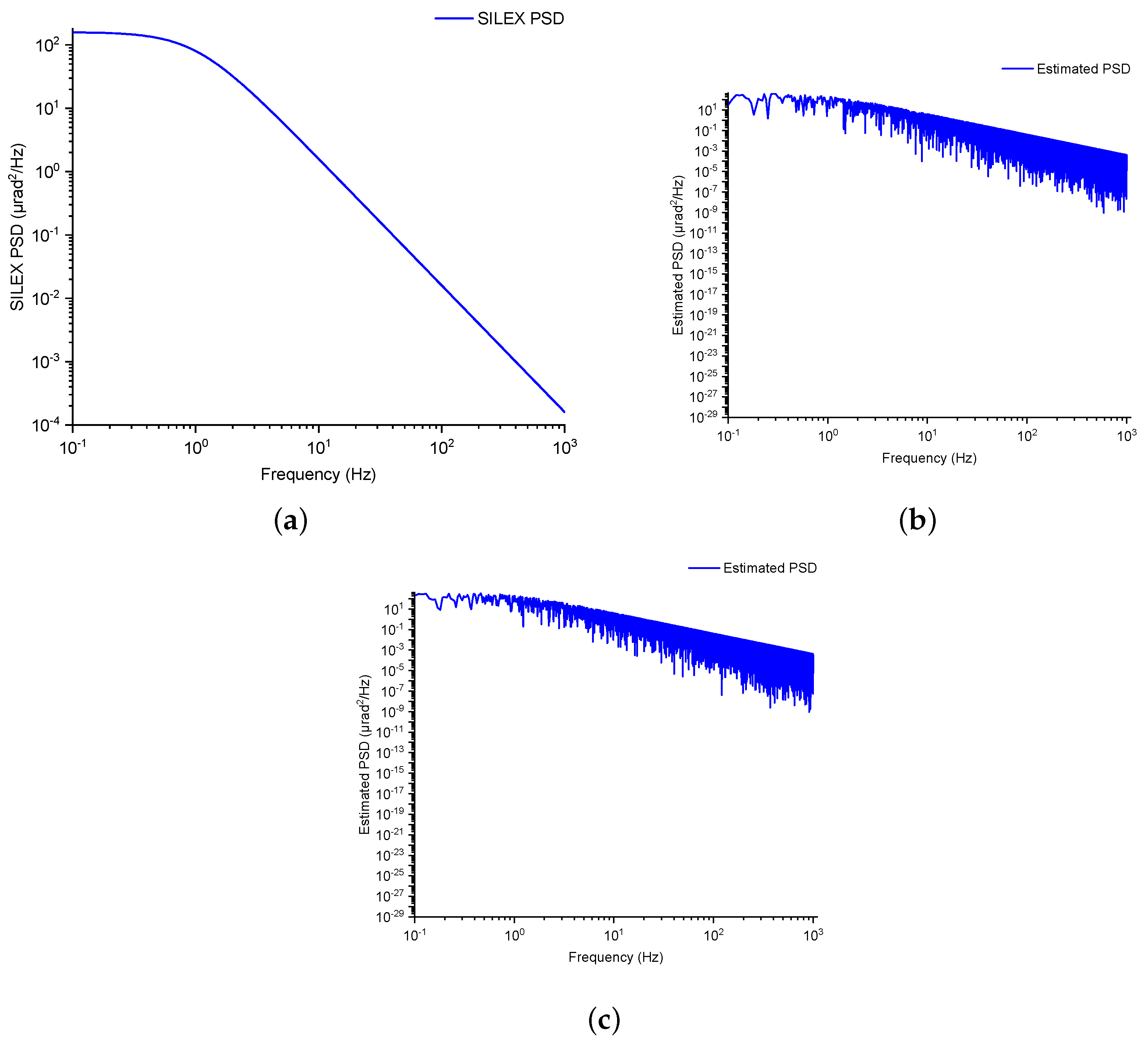
4.1. Power Spectral Density

The characteristics of the satellite platform vibrations can be studied using the power spectral model used by the European Space Agency (ESA) during the SILEX program, as given below [49,50,51]:
S ( f ) = 160 μ ra d 2 / Hz 1 + f 2 ,
where f represents the vibration frequency. As depicted in Figure 7a, the spectrum of the vibrations is concentrated in the low-frequency range, with high amplitudes at lower frequencies and lower power at higher frequencies. Figure 7b shows the corresponding time-domain signal of the pointing error between the transmitter and the receiver satellite, obtained after applying random phases to the power spectral density (PSD) components with a standard deviation of 10 μrad. The PSD can be used to generate infinite time-domain signals for simulation studies.

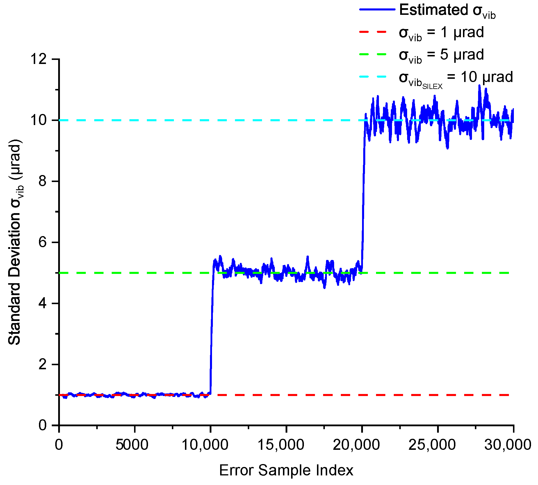
4.2. Maximum Likelihood Estimation (MLE) of Vibration Error

The onboard accelerometer can measure vibration amplitude samples for the pointing error in both the horizontal (x) and vertical (y) directions [48,52]. It is assumed that these x and y samples are independent and identically distributed (i.i.d.) zero-mean Gaussian random variables with the same variance. Then, the radial pointing error R can be computed as follows:
R = X 2 + Y 2 .
Since R represents the magnitude of a two-dimensional vector formed by independent Gaussian-distributed variables, it follows a Rayleigh distribution. The PDF of the Rayleigh distribution for the random variable R is given by
f R ( r ) = r σ vib exp r 2 2 σ vib 2 ,
where σ vib is the standard deviation of the optical beam’s displacement due to platform vibration. To estimate the standard deviation σ vib of the optical beam’s displacement due to platform vibration from the observed data R i , the MLE method can be employed. MLE is a statistical method used to estimate the parameters of a probability distribution based on observed data. The principle behind MLE is to find the parameter values that maximize the likelihood function, which represents the probability of observing the given data under different parameter values.
The MLE for the standard deviation σ vib of a Rayleigh distribution can be derived by maximizing the likelihood function, and the expression for the estimation of σ vib can be written as follows [53,54]:
σ ^ vib = 1 2 m i = 1 m R i 2 ,
where R i = X i 2 + Y i 2 are the radial pointing error values calculated for each sample in a given window, and m is the number of samples in the window.
Due to the dynamic nature of the satellite platform’s vibration environment, a sliding window approach can be applied to estimate the standard deviation σ vib to suit the dynamic nature of the laser link communication environment. This allows the estimator to adapt to changes in the platform’s vibrational characteristics over time. The sliding window size can be varied, and the standard deviation σ vib can be estimated using the MLE method described above.
In this method, the basic steps are as follows. For each sliding window of size w, the radial errors R i can be calculated for the corresponding X i and Y i values. The MLE for σ vib can then be computed and updated for each new window position as the window moves through the dataset. This approach provides a dynamic estimation of the standard deviation of the radial pointing error.

5. Optimization of Scan Parameters
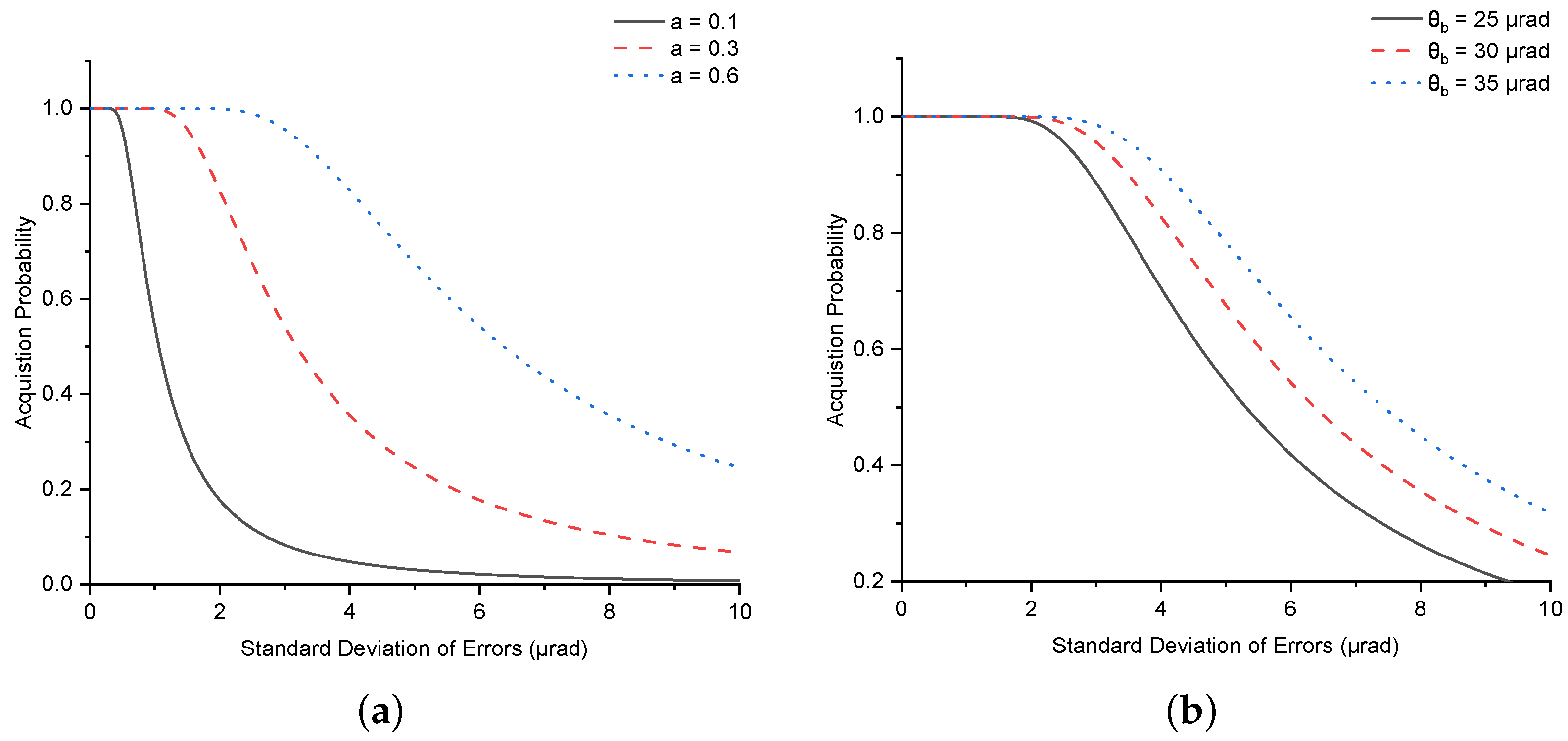
During the acquisition phase of the APT process to establish the inter-satellite laser link, in the presence of satellite platform vibrations, the scan parameters that can be varied are the overlap factor a, the beam divergence θ b , and the uncertainty area θ area [40]. The primary objective is to reduce the scan time while increasing the acquisition probability in the presence of jitter.

5.1. Overlap Factor

Scanning the uncertainty area is performed using a step size n, which defines the scan spots (or dwell points). To ensure a safety margin against jitter, an overlap factor is introduced into the step size, as defined in Equation (12), where a is the overlap factor, and θ b is the beam divergence that illuminates a portion of the uncertainty area at each spot. The presence of satellite platform vibrations can result in missed target scan spots, causing either excessive overlap or missed scan areas. The LOS link between the transmitter and receiver satellites is subject to jitter, leading to pointing errors. Since the radial pointing error follows a Rayleigh distribution, its probability density function can be written as
f ( γ ) = γ σ vib exp γ 2 2 σ vib 2 ,
where γ is the deviation from the intended scan spot, and σ vib is the standard deviation of the scanning beam due to vibrations. When γ exceeds a certain threshold α in both the elevation and azimuth directions, scan gaps are created. Therefore, the probability P m of missing a scan spot can be derived as follows [40]:
P m = α f ( γ ) d γ ,
P m = α γ σ vib exp γ 2 2 σ vib 2 d γ = exp α 2 2 σ vib 2 .
Thus, the acquisition probability P c , which represents the probability of successfully acquiring the scan spot (i.e., the scan point remaining within the acceptable threshold), can be written as
P c = 1 P m = 1 exp α 2 2 σ vib 2
The limit for the pointing error deviation α can be expressed using Equation (72) as
α = σ vib 2 ln ( 1 P c ) .
To ensure that there are no gaps between the scan beam footprint when scanning each point, the step distance n must satisfy the following condition:
n θ b 2 α .
Substituting n = θ b ( 1 a ) into the inequality, we obtain
θ b ( 1 a ) θ b 2 α .
By simplifying this inequality, we can express the required overlap factor a as follows:
1 a θ b 2 α θ b ,
a 2 α θ b .
Finally, substituting α = σ vib 2 ln ( 1 P c ) in Equation (77), we can derive the final expression for a:
a 2 σ vib 2 ln ( 1 P c ) θ b .
To avoid missed scan areas and gaps, the overlap factor must satisfy the condition in Equation (78).

5.2. Beam Divergence

Beam divergence is another scanning parameter that can be adjusted to mitigate the impact of satellite vibrations and avoid creating scan gaps while scanning the uncertainty area [55]. By adaptively changing the beam divergence based on the magnitude of vibrations, the system can maintain alignment and minimize performance degradation. This approach, known as the Adaptive Beam Control (ABC) technique, has been extensively studied and demonstrated in various scenarios. ABC enables the dynamic adjustment of beam divergence at both the transmitter and receiver to respond to changing channel conditions, such as pointing errors and angle-of-arrival (AoA) fluctuations [56,57].
ABC can be implemented in two main forms: static ABC and dynamic ABC. Static ABC adjusts beam parameters based on pre-determined statistical information about the channel conditions, such as average pointing errors or AoA fluctuations and operates on slower timescales [58,59,60]. In contrast, dynamic ABC responds in real time to instantaneous feedback from rate sensors, making it more effective in mitigating rapid variations caused by satellite vibrations [61,62]. Various techniques have been developed to implement ABC, each offering distinct mechanisms to optimize beam divergence and focus.
One approach involves the use of optical switches to select between multiple emitters or detectors with predefined beam divergence angles or radii. While simple in concept, this method suffers from slow response times and limited adaptability, making it unsuitable for real-time dynamic adjustments [63]. Another method employs mechanically adjustable lenses, where the lens position relative to the emitter or detector is modified to control the beam’s divergence or focus. Although this technique offers more flexibility than optical switches, it is prone to mechanical failure, slower adjustment speeds, and higher implementation costs [64].
In contrast, the Variable Focus Lens (VFL) provides a more advanced solution for ABC [65,66]. VFLs adjust the beam’s focal length electronically using electrowetting or electromagnetic actuation, enabling precise, non-mechanical, and millisecond-scale adjustments [67,68]. This approach is particularly advantageous for dynamic ABC systems, where real-time feedback from rate sensors is used to counteract pointing errors and AoA fluctuations. Additionally, the VFL-based technique can be enhanced by employing a double-lens configuration, which overcomes the aperture size limitations of VFLs and enables simultaneous beam optimization at both the transmitter and receiver.
For the given parameters, i.e., overlap factor a, satellite vibration standard deviation σ vib , and acquisition probability P c , the required beam divergence to avoid scan gaps can be calculated using Equation (78) as follows:
θ b 2 σ vib 2 ln ( 1 P c ) a .

5.3. Uncertainty Area Size

The uncertainty area size can also be varied during the scanning phase. There is an initial offset error σ that exists between the transmitter and receiver satellites, which arises due to pointing errors, satellite attitude, thermal distortions, and ephemeris data. However, as demonstrated by the authors in [40], changing the uncertainty area size without altering the overlap factor or the beam divergence in the presence of vibrations does not reduce the scan gaps. Nevertheless, in terms of the mean acquisition time, two different values, i.e., u = 3 σ or u = 1.3 σ , can be used.
Since the radial error follows a Rayleigh distribution according to Equation (9), the acquisition probability P s of the target receiver satellite appearing in the uncertainty region can be obtained by integrating Equation (17) as
P s = 0 u f ( r ) d r = 1 exp u 2 2 σ 2 ,
where u is half the size of the uncertainty area.
Figure 8 depicts the acquisition probability versus the ratio u σ . This demonstrates that setting u = 3 σ is sufficiently large to cover the probable positions of the target satellite and acquire it with a probability exceeding 98%. The authors in [46] suggested and demonstrated that the optimum uncertainty area size, u = 1.3 σ , is better than the traditional approach, especially at larger values of σ .

6. Simulation Results and Discussion

This section presents the simulation results for the mean acquisition time of the scanning methods: spiral, raster, square spiral, and hexagon. The dwell time, Δ t , and the beam divergence, θ b , were set to 0.1 s and 25 microradians, respectively, for different values of the standard deviation of the satellite’s position and the size of the uncertainty area to be scanned during the simulations. The satellite platform vibration model by ESA and NASDA were utilized to generate random vibration signals for the standard deviation estimation using a sliding window [69]. For all the computations, Python version 3.12.3 and MATLAB version 9.7.0.1190202 (R2019b) were utilized.

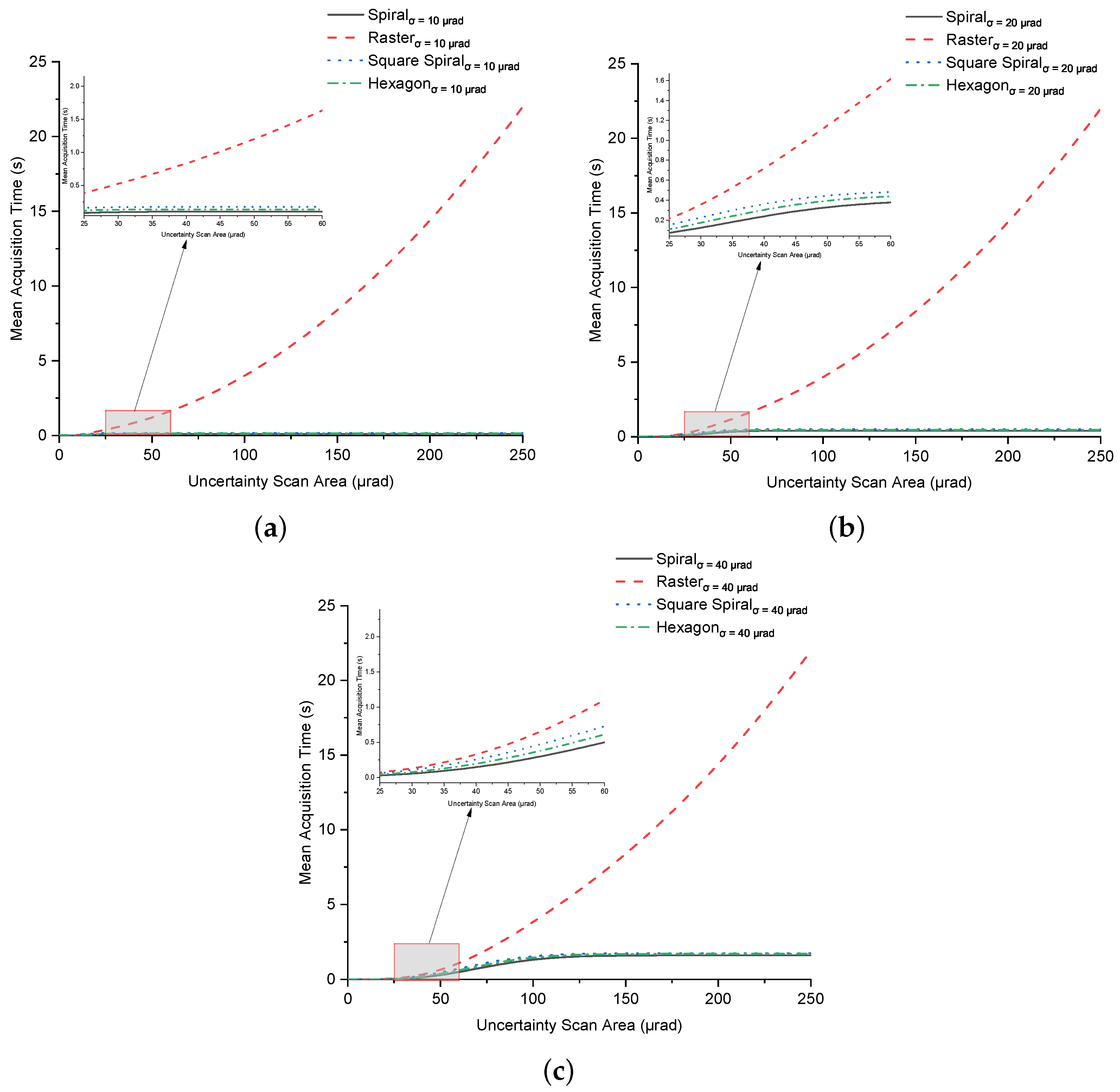
6.1. Mean Acquisition Time Using Spiral Scan

Figure 9a,b illustrate the mean acquisition time E T s and its relationship with the field of uncertainty (FOU) area and the satellite position’s standard deviation, respectively, when the spiral scan method is employed. The acquisition time E T s increases with the size of the scan area and the error in the satellite’s position. Specifically, E T s is approximately [0.09, 0.36, 1.45] seconds for σ = [ 10 , 20 , 40 ] μrad, corresponding to 98% coverage of the uncertainty area, respectively. As expected, the time required to scan the uncertainty area increased as the receiver satellite moved farther from the center. This is because the spiral scan begins from the center, where the highest probability of locating the target satellite exists, and progressively moves toward the lower-probability regions near the edges. The relationship between the acquisition probability and the uncertainty area is described by the following equation:
θ area = 2 u = σ 2 ln ( 1 P c ) ,
where σ is the satellite position’s standard deviation, and P c is the desired acquisition probability, set to 0.98. It is evident that reducing the scan area size will decrease the acquisition time; however, this comes at the cost of lowering the acquisition probability, which could result in multiple scans of the uncertainty area.

6.2. Mean Acquisition Time Using Raster Scan

Figure 10a depict the mean acquisition time E T r to scan the uncertainty area when the raster scan method is used for various standard deviations of the receiver satellite position error. As expected, the curves show behavior corresponding to the scan path. For the same value of uncertainty scan area, i.e., 50 μrad, E T r is approximately [0.38, 0.21, 0.07] seconds for σ = [ 10 , 20 , 40 ] μrad, respectively. This behavior is clearly illustrated in Figure 10b, where the mean acquisition time decreases as the receiver satellite moves away from the center, and vice versa. The scan time decreases as the satellite moves away from the center, from regions of high probability to regions of low probability. Since the raster scan begins at the edges (low probability) and scans the area in a zigzag fashion toward the center (high probability), the curves eventually converge to the time required for the entire square area to be scanned by the raster scan. The acquisition time E T r increases with the size of the scan area but decreases with an increase in the standard deviation of the satellite’s position. Specifically, E T r is approximately [0.46, 1.42, 4.80] seconds for σ = [ 10 , 20 , 40 ] μrad when P c is set to 0.98 in Equation (81).

6.3. Mean Acquisition Time Using Square Spiral Scan

Figure 11a,b depict the performance of the square spiral scan method, which combines the properties of both spiral and raster scanning. The square spiral scan begins from the region of high probability (the center) and moves towards the region of low probability (the edges) of the scan area. The mean acquisition time, E T ss , is approximately [0.16, 0.47, 1.64] seconds for σ = [ 10 , 20 , 40 ] μrad as the size of the uncertainty area increases. The square spiral extends outward in discrete squares, efficiently covering the entire uncertainty area. As expected, E T ss is smaller when the satellite position error is small and increases as the satellite is farther from the center, as depicted in Figure 11b.

6.4. Mean Acquisition Time Using Hexagon Scan

Figure 12a,b display the mean acquisition time when the scanning method follows a hexagonal path. Similar to a spiral scan, the path begins at the center (high probability) and extends outward to the low-probability region. The mean acquisition time E T h values are [0.13, 0.43, 1.58] seconds for σ values of [10, 20, 40] μrad, for various FOU values. The time required to scan the area increased as the standard deviation increased, as seen in Figure 12b, as expected due to the target satellite position’s probability distribution.

6.5. Error Estimation for Satellite Vibration Effects

Figure 13a shows the PSD of the satellite platform vibration model used by ESA during the SILEX program, as described by Equation (65) for the specified frequency range. This model can be used for satellite vibration analysis and to generate vibration signals in both the vertical and horizontal directions. Figure 13b,c show the estimated PSDs for the vibration signals in the vertical and horizontal directions, respectively. The estimated PSD is consistent with the PSD model shown in Figure 13, validating its use for generating vibration signals in both directions. These signals were used to compute the radial vibration signal and to ultimately estimate the standard deviation using the sliding window method, as depicted in Figure 14.
The algorithm to generate time-series data from the PSD involves seven steps. The first step is to define the time length of the time-series data, which is then used to retrieve the frequency resolution. The second step is to define the desired frequency range. To generate the time array, a sampling frequency is required, which can be calculated using the final frequency of the PSD curve according to the Nyquist theorem. The third step involves sampling the PSD curve within the selected range. The fourth step is to compute the single-sided and normalized amplitude of the discrete Fourier transform (DFT). To build the time-series data, phase information is also needed, which is absent in the power spectral density; therefore, in the fifth step, random phases are generated for each value of the DFT. This step is crucial as it enables the creation of infinite time-domain signals. The sixth step is to retrieve the DFT coefficients in both real and imaginary formats. The final step is to compute the inverse DFT to generate the time-domain vibration signals in both vertical and horizontal directions.
Figure 14 illustrates the performance of the maximum likelihood estimator using a sliding window of size 200 to estimate different standard deviations, i.e., σ vib = [ 1 , 5 , 10 ] μrad, where σ vib = 10 μrad is associated with the PSD model described in Equation (65). The estimator’s performance is quite stable with the current window size, as the errors in both the vertical and horizontal directions are independent and identically distributed (i.i.d.) Gaussian random variables with zero mean and the same variance. The estimation accuracy, evaluated using the root mean square error (RMSE), was [0.03, 0.3, 0.5] μrad for σ vib = [ 1 , 5 , 10 ] μrad, respectively. These RMSE values confirm that the estimator maintains reliable performance across varying standard deviations, with minimal deviation around each target value.

6.6. Impact of Scan Parameters on Acquisition Performance

Figure 15a illustrates the impact of selecting the overlap factor on acquisition performance. The overlap factor, which is directly related to the scanning step size n, plays a crucial role in avoiding gaps during the scanning process. Specifically, a higher overlap factor reduces the risk of missing regions within the scanning area, which is essential for achieving high acquisition probabilities in the presence of jitter. Given the beam divergence, the pointing error deviation of the satellite due to vibrations, and the acquisition probability of 0.98 for this simulation, the necessary overlap factor can be calculated using Equation (78), and its relationship with the acquisition probability is shown in Figure 15a.
As depicted, acquisition probability declines with an increase in σ vib , which represents the standard deviation of errors caused by satellite vibrations. This decline in acquisition probability can, however, be mitigated by increasing the overlap factor, effectively compensating for the increased positional uncertainty caused by vibrations. This result underscores the importance of adjusting the overlap factor based on expected error magnitudes to maintain optimal acquisition performance.
Figure 15b shows a similar trend when the overlap factor is fixed and the beam divergence is varied. Here, the acquisition probability decreases as σ vib increases, but this effect can be countered by increasing the beam divergence. Adjusting beam divergence is, thus, another viable approach to maintaining the acquisition probability when a fixed overlap factor is used.
Overall, these findings suggest that optimizing the selection of both the overlap factor and beam divergence, particularly in scenarios with significant pointing and jitter errors induced by satellite platform vibrations, can minimize the need for multiple scans of uncertain areas and enhance the acquisition probability within a single scan. Proper selection of these parameters is crucial for robust performance in satellite-based scanning applications where uncertainty is a factor.

6.7. Discussion

Figure 16 presents a comparative analysis plot of four distinct scanning methods: spiral, raster, square spiral, and hexagonal. The mean acquisition time is plotted for increasing uncertainty areas across different σ values. These results provide insight into the efficiency of each scanning method in terms of mean acquisition time relative to the probability distribution of the receiver satellite’s position.
Among the four methods, the spiral, square spiral, and hexagonal scans start at the high-probability region and proceed outward toward areas of lower probability. This prioritization leads to reduced acquisition times as these scans effectively target the most probable areas first. In contrast, the raster scan initiates at a lower-probability region and progresses towards the high-probability region, which extends the overall acquisition time. Consequently, the raster scan demonstrates the longest acquisition time among the methods. Ranking the four scanning methods, the mean acquisition times follow this order: spiral < hexagonal < square spiral < raster.
The square spiral and spiral scans both commence scanning from the center, quickly addressing high-probability areas, with the square spiral being more suited to square-shaped uncertainty regions. The hexagonal scan also begins at the center; however, due to its geometry, some scan points fall outside the square region, potentially reducing its efficiency in fully covering the square uncertainty area. The raster scan, by starting from an edge, further delays coverage of these central, high-probability zones.
In evaluating these metrics, the square spiral scan is shown to be particularly effective for square uncertainty areas, as it ensures complete and efficient coverage. The raster scan, while covering the entire area, is less efficient in prioritizing areas based on probability. The hexagonal scan may leave unscanned gaps along the edges due to alignment mismatches with square-shaped regions, and the spiral scan, due to its circular pattern, might leave portions of the square uncertainty area unscanned. However, since the spiral path aligns well with the possible positions of the target satellite within the uncertainty scan area, as illustrated for each path in Figure 17, the spiral scan method is more efficient in terms of both the least mean acquisition time and the number of scan points required to cover the uncertainty region with the highest probability of locating the target satellite. The scan points required by these four methods to cover the uncertainty area θ area = ± 250 μrad (see Figure 17) differ. The square spiral and hexagonal scan methods also focus on the high-probability area; however, the overall number of scan points required is greater than that of the spiral scan method.
In terms of mechanical implementation, the four scan paths—raster, square spiral, spiral, and hexagonal—require different approaches. The raster scan involves linear movements and straightforward directional changes. The square spiral scan combines straight-line movements with periodic directional shifts. The spiral scan requires smooth, continuous curved trajectories to maintain consistent motion. The hexagonal scan demands precise path calculations to ensure efficient coverage due to its angular and non-linear pattern. Each path has unique implementation requirements that influence how it is designed and executed.
The availability of a power spectral density model for satellite and spacecraft vibrations is crucial for analyzing vibration sources and leveraging these insights in simulation studies. This model supports various functions, including testing different PSD regeneration techniques, validating the accuracy of regenerated PSD against the original model, and generating vibration time-domain signals for further analysis. In this study, time series data were used in the maximum likelihood estimator through a sliding window technique to accurately estimate the standard deviation σ vib of the satellite platform vibrations (see Figure 13 and Figure 14).
Figure 13a shows the original PSD model, presenting a clear baseline for comparison with the estimated results in Figure 13b,c. These estimates, derived using an algorithm, effectively capture the frequency distribution characteristics, validating the algorithm’s accuracy in regenerating PSD signals. In Figure 13b,c, the estimated PSD curves closely align with the original PSD, indicating a high level of precision in the estimation process.
The sliding window technique, illustrated in Figure 14, plays a critical role in ensuring robust and dynamic σ vib estimation. By using samples of the vibration signal magnitudes from both the x and y directions and focusing on the most recent data, this approach enables decision-making based on current conditions. This method enhances the stability of the maximum likelihood estimator, contributing to a smoother and more accurate σ vib estimation.
These results collectively demonstrate that the PSD model and the proposed estimation methodology provide a reliable basis for simulating satellite and spacecraft vibration characteristics. The alignment between the estimated PSD and the original model suggests that the sliding window technique, combined with maximum likelihood estimation, offers an effective approach to σ vib estimation in inter-satellite laser link applications.
During the acquisition phase of establishing an inter-satellite laser link, precision is hindered by satellite platform vibrations. To minimize the impact of such vibrations on successful acquisition and to avoid multiple scans of the same uncertainty area, several scan parameters can be optimized, including overlap factor, beam divergence, and the size of the uncertainty area, as reported in [40]. In the presence of vibrations, changing the uncertainty area alone, while keeping the beam divergence and overlap factor constant, did not reduce scan gaps. Therefore, optimizing both the overlap factor and beam divergence is essential in the presence of vibrations.
The optimization of these scan parameters depends on an accurate estimation of σ vib , whose performance is displayed in Figure 14. In addition to the estimation accuracy, the overlap factor and beam divergence have inherent limitations, as varying these parameters impacts scanning time. Thus, optimal performance represents an interplay between these factors.
Figure 18 illustrates the performance of the spiral scan method under satellite platform vibrations, comparing fixed and optimized scan parameters. Figure 18a,b depict the spiral scan path and its perturbation due to vibrations with σ vib = 5 μrad, where Monte Carlo simulations were conducted using an overlap factor a = 0.2 and beam divergence θ b = 25 μrad. The results in Figure 18c,d show that the fixed parameters resulted in an average of 1.23 scans with a variance of 0.78, and a mean scan time of 9.38 s with a variance of 30.51 s.
In contrast, Figure 18e,f highlight the improvements achieved by optimizing a and θ b based on the estimated satellite vibrations. The range of a was 0 a 0.9 , and θ b ranged from 25 μrad to 35 μrad. This optimization reduced the number of scans and the total scan time significantly, achieving a mean of 1.01 scans with a variance of 0.10, and a mean scan time of 0.88 s with a variance of 4.49 s. These results demonstrate the effectiveness of adapting scan parameters to vibration conditions to enhance the detection probability and minimize scan gaps.
The results collectively emphasize that optimal acquisition performance represents an interplay between these scan parameters and scan paths, where careful tuning of overlap factor and beam divergence is essential. By achieving this balance, the system can maintain a high acquisition accuracy while minimizing scan duration, even in the presence of satellite vibrations. The findings offer practical insights into parameter selection strategies that improve acquisition reliability and efficiency in inter-satellite laser link applications.

7. Conclusions

Optical wireless communication (OWC) has emerged as a key alternative to traditional RF communication, offering a higher bandwidth, faster data rates, and lower power consumption. A line-of-sight (LOS) laser link is established through the acquisition, pointing, and tracking (APT) system to initiate communication, which faces challenges due to satellite vibrations.
In this study, several scanning paths were evaluated based on their mean acquisition time, and the results showed the following performance ranking: spiral < hexagonal < square spiral < raster. Based on the analysis, spiral scanning is the best method among the discussed techniques. It offers the highest scanning efficiency by starting from the high-probability center region, enabling faster target detection. In addition to selecting the scan path, adjusting scan parameters such as the overlap factor can increase acquisition probability, although it also increases acquisition time. Modifying the beam divergence in the presence of vibrations can reduce scan gaps, whereas changing the uncertainty area size, without altering the overlap factor or beam divergence, does not reduce the scan gaps.
By optimizing these multiple scan parameters and selecting the appropriate scan path, an effective trade-off between acquisition time and acquisition probability can be achieved, provided that the satellite vibration amplitudes do not exceed the limitations imposed by the scan parameters. Monte Carlo simulations revealed that optimized parameters reduced the need for repeated scans to almost none (1.01 scans on average), compared to 1.23 scans with fixed parameters, and achieved a remarkable 90.6% reduction in scan time (from 9.38 s to 0.88 s). This underscores the effectiveness of parameter optimization in minimizing both scan repetitions and acquisition time under satellite vibrations. The performance of the maximum likelihood estimator was also found to be reliable. Future studies should explore additional scan methods, including Rose and Lissajous paths, and evaluate them using probabilistic approaches. An enhanced estimation of satellite vibrations should be considered to improve the robustness of scan parameter performance in the acquisition phase.

Author Contributions

Conceptualization, W.J.; methodology, M.K.; software, M.K.; validation, W.J., D.L. and L.K.; investigation, M.K.; data curation, M.K.; writing—original draft preparation, M.K.; writing—review and editing, M.K., W.J., D.L. and L.K.; visualization, M.K.; supervision, W.J.; project administration, W.J.; funding acquisition, W.J. All authors have read and agreed to the published version of the manuscript.

Funding

This research was funded by the National Key R&D Program of China (Grant No. 2021YFB3900100) and the Beijing Municipal Science and Technology (Grant No. Z241100005424008).

Institutional Review Board Statement

Not applicable.

Informed Consent Statement

Not applicable.

Data Availability Statement

Data are contained within the article.

Acknowledgments

The author Muhammad Khalid acknowledges the support of the Alliance of International Science Organizations (ANSO) Scholarship for Young Talents series No. 2021ANSOP050 during the research for this study.

Conflicts of Interest

The authors declare no conflicts of interest.

Abbreviations

The following abbreviations are used in this manuscript:
ABCAdaptive Beam Control
LOSLine-of-sight
ESAEuropean Space Agency
GPSGlobal Positioning System
IoTInternet of Things
MLEMaximum Likelihood Estimation
OWCOptical Wireless Communication
PAAPoint Ahead Angle
APTAcquisition Pointing and Tracking
VFLVariable Focus Lens
BERBit Error Rate
DFTDiscrete Fourier Transform
FOUField of Uncertainty
FOVField of View
PSDPower Spectral Density
PDFProbability Density Function
RMSERoot Mean Square Error

Appendix A

For subdomain I a in Figure A1, the variable y ranges from u to n u . When y is fixed, x ranges from y to u.
Figure A1. Subdomain I a .
Photonics 12 00444 g0a1
Hence, the integral for subdomain I a is
I a = u n u y u T ss ( x , y ) f ( x , y ) d x d y .
From Equations (33) and (34), we know that T ss ( x , y ) = L ss ( x , y ) n · Δ t . Additionally, from Equation (30), S M = 8 n M ( M + 1 ) 2 , and from Equation (31), M = x n . Therefore, the value of L a on subdomain I a is
L a ( x , y ) = S M + x M n .
Substituting for S M and M:
L a ( x , y ) = 8 n x n x n + 1 2 + x x n n .
Thus, the expression for L a ( x , y ) becomes
L a ( x , y ) = 4 n x n 2 + 3 n x n + x .
Therefore,
I a = u n u y u 4 x x n + 1 Δ t 2 π n σ 2 exp 1 2 x 2 + y 2 σ 2 d x d y .
For subdomain I b in Figure A2, the variable y ranges from n u to 0. When y is fixed, x ranges from y to n y . This can be seen by considering the Cartesian equations of both diagonals, which have slopes of 1 and intercepts of 0 and n, respectively.
Figure A2. Subdomain I b .
Photonics 12 00444 g0a2
Since the value of L b remains the same as before, we obtain
I b = n u 0 y n y 4 x x n + 1 Δ t 2 π n σ 2 exp 1 2 x 2 + y 2 σ 2 d x d y .
For subdomain I c in Figure A3, the variable y ranges from 0 to n 2 . When y is fixed, x ranges from y to n y .
Figure A3. Subdomain I c .
Photonics 12 00444 g0a3
Since the value of L c remains the same as before, we obtain
I c = 0 n 2 y n y 4 x x n + 1 Δ t 2 π n σ 2 exp 1 2 x 2 + y 2 σ 2 d x d y .
For domain I 2 in Figure A4, the variable x ranges from n 2 to u. When x is fixed, y ranges from n x to x.
Figure A4. Domain I 2 .
Photonics 12 00444 g0a4
Hence, the integral for domain I 2 is
I 2 = n 2 u n x x T ss ( x , y ) f ( x , y ) d y d x .
In domain I 2 , we have x 0 and | x | | y | , so M = x n . Therefore, the value of L 2 on domain I 2 is
L 2 ( x , y ) = S M 1 + M n + y .
Substituting for S M 1 and M:
L 2 ( x , y ) = 4 n x n x n 1 + x n n + y .
Thus, the expression for L 2 ( x , y ) becomes
L 2 ( x , y ) = 4 n x n 2 3 n x n + y .
Finally, we obtain
I 2 = n 2 u n x x 4 x 2 n 3 x + y Δ t 2 π n σ 2 exp 1 2 x 2 + y 2 σ 2 d y d x .
For domain I 3 in Figure A5, the variable y ranges from 0 to u. When y is fixed, x ranges from y to y.
Figure A5. Domain I 3 .
Photonics 12 00444 g0a5
Hence, the integral for domain I 3 is
I 3 = 0 u y y T ss ( x , y ) f ( x , y ) d x d y .
In domain I 3 , we have y 0 and | y | | x | , so M = y n . Therefore, the value of L 3 on domain I 3 is
L 3 ( x , y ) = S M 1 + 3 M n x .
Substituting for S M 1 and M:
L 3 ( x , y ) = 4 n y n y n 1 + 3 y n n x .
Thus, the expression for L 3 ( x , y ) becomes
L 3 ( x , y ) = 4 n y n 2 n y n x .
Finally, we obtain
I 3 = 0 u y y 4 y 2 n y x Δ t 2 π n σ 2 exp 1 2 x 2 + y 2 σ 2 d x d y .
For domain I 4 in Figure A6, as x varies from u to 0, y varies from x to x . Hence, the integral for domain I 4 is
I 4 = u 0 x x T ss ( x , y ) f ( x , y ) d y d x .
Figure A6. Domain I 4 .
Photonics 12 00444 g0a6
In domain I 4 , we have x 0 and | x | | y | . Therefore, M = x n . Thus, the value of L 4 on domain I 4 is
L 4 ( x , y ) = S M 1 + 5 M n y .
Substituting for S M 1 and M, we obtain
L 4 ( x , y ) = 4 n x n x n 1 + 5 x n n y .
Therefore, the expression for L 4 ( x , y ) becomes
L 4 ( x , y ) = 4 n x n 2 + n x n y .
Finally, we obtain
I 4 = u 0 x x 4 x 2 n x y Δ t 2 π n σ 2 exp 1 2 x 2 + y 2 σ 2 d y d x .
For domain I 5 in Figure A7, as y varies from u to 0, x varies from y to y . Hence, the integral for domain I 5 is
I 5 = u 0 y y T ss ( x , y ) f ( x , y ) d x d y .
Figure A7. Domain I 5 .
Photonics 12 00444 g0a7
In domain I 5 , we have y 0 and | y | | x | . Therefore, M = y n . Thus, the value of L 5 on domain I 5 is
L 5 ( x , y ) = S M 1 + 7 M n + x .
Substituting for S M 1 and M, we obtain
L 5 ( x , y ) = 4 n y n y n 1 + 7 y n n + x .
Therefore, the expression for L 5 ( x , y ) becomes
L 5 ( x , y ) = 4 n y n 2 + 3 n y n + x .
Finally, we obtain
I 5 = u 0 y y 4 y 2 n 3 y + x Δ t 2 π n σ 2 exp 1 2 x 2 + y 2 σ 2 d x d y .

References

  1. Raj, A.B.; Majumder, A.K. Historical perspective of free space optical communications: From the early dates to today’s developments. IET Commun. 2019, 13, 2405–2419. [Google Scholar] [CrossRef]
  2. Raj, A.A.B.; Krishnan, P.; Darusalam, U.; Kaddoum, G.; Ghassemlooy, Z.; Abadi, M.M.; Majumdar, A.K.; Ijaz, M. A Review–Unguided Optical Communications: Developments, Technology Evolution, and Challenges. Electronics 2023, 12, 1922. [Google Scholar] [CrossRef]
  3. Jahid, A.; Alsharif, M.H.; Hall, T.J. A contemporary survey on free space optical communication: Potentials, technical challenges, recent advances and research direction. J. Netw. Comput. Appl. 2022, 200, 103311. [Google Scholar] [CrossRef]
  4. Kaushal, H.; Kaddoum, G. Optical Communication in Space: Challenges and Mitigation Techniques. IEEE Commun. Surv. Tutor. 2017, 19, 57–96. [Google Scholar] [CrossRef]
  5. Zafar, S.; Khalid, H. Free Space Optical Networks: Applications, Challenges and Research Directions. Wirel. Pers. Commun. 2021, 121, 429–457. [Google Scholar] [CrossRef]
  6. Khalighi, M.A.; Uysal, M. Survey on Free Space Optical Communication: A Communication Theory Perspective. IEEE Commun. Surv. Tutor. 2014, 16, 2231–2258. [Google Scholar] [CrossRef]
  7. Sova, R.M.; Sluz, J.E.; Young, D.W.; Juarez, J.C.; Dwivedi, A.; Demidovich, N.M., III; Graves, J.E.; Northcott, M.; Douglass, J.; Phillips, J.; et al. 80 Gb/s free-space optical communication demonstration between an aerostat and a ground terminal. In Proceedings of the Free Laser Communication VI, San Diego, CA, USA, 1 September 2006; SPIE: St Bellingham, WA, USA, 2006; Volume 6304, p. 630414. [Google Scholar] [CrossRef]
  8. Gregory, M. Commercial optical inter-satellite communication at high data rates. Opt. Eng. 2012, 51, 031202. [Google Scholar] [CrossRef]
  9. Zhang, X.; Klevering, G.; Lei, X.; Hu, Y.; Xiao, L.; Tu, G.H. The Security in Optical Wireless Communication: A Survey. ACM Comput. Surv. 2023, 55, 3594718. [Google Scholar] [CrossRef]
  10. Kodheli, O.; Lagunas, E.; Maturo, N.; Sharma, S.K.; Shankar, B.; Montoya, J.F.M.; Duncan, J.C.M.; Spano, D.; Chatzinotas, S.; Kisseleff, S.; et al. Satellite Communications in the New Space Era: A Survey and Future Challenges. IEEE Commun. Surv. Tutor. 2021, 23, 70–109. [Google Scholar] [CrossRef]
  11. Liu, W.; Ding, J.; Zheng, J.; Chen, X.; Lin, C. Relay-Assisted Technology in Optical Wireless Communications: A Survey. IEEE Access 2020, 8, 194384–194409. [Google Scholar] [CrossRef]
  12. Liang, J.; Chaudhry, A.U.; Erdogan, E.; Yanikomeroglu, H.; Kurt, G.K.; Hu, P.; Ahmed, K.; Martel, S. Free-Space Optical (FSO) Satellite Networks Performance Analysis: Transmission Power, Latency, and Outage Probability. IEEE Open J. Veh. Technol. 2024, 5, 244–261. [Google Scholar] [CrossRef]
  13. Dmytryszyn, M.; Crook, M.; Sands, T. Lasers for Satellite Uplinks and Downlinks. Science 2021, 3, 4. [Google Scholar] [CrossRef]
  14. Chaudhry, A.U.; Yanikomeroglu, H. Temporary Laser Inter-Satellite Links in Free-Space Optical Satellite Networks. IEEE Open J. Commun. Soc. 2022, 3, 1413–1427. [Google Scholar] [CrossRef]
  15. Hamza, A.S.; Deogun, J.S.; Alexander, D.R. Classification Framework for Free Space Optical Communication Links and Systems. IEEE Commun. Surv. Tutor. 2019, 21, 1346–1382. [Google Scholar] [CrossRef]
  16. Devkota, N.; Maharjan, N.; Kim, B.W. Atmospheric Effects on Downlink Channel of Satellite to Ground Free Space Optical Communications. In Proceedings of the 2022 13th International Conference on Information and Communication Technology Convergence (ICTC), Jeju Island, Republic of Korea, 19–21 October 2022; IEEE: Piscataway, NJ, USA, 2022; Volume 2022, pp. 1335–1340. [Google Scholar] [CrossRef]
  17. Tiwari, G. A Review on Inter-Satellite Links Free Space Optical Communication. Indian J. Sci. Technol. 2020, 13, 712–724. [Google Scholar] [CrossRef]
  18. Khalid, M.; Ji, W.; Li, D.; Kun, L. Characterization of Doppler shift in inter-satellite laser link between LEO, MEO, and GEO orbits. Opt. Laser Technol. 2024, 177, 111033. [Google Scholar] [CrossRef]
  19. Kaushal, H.; Jain, V.K.; Kar, S. Acquisition, Tracking, and Pointing; Springer: Berlin/Heidelberg, Germany, 2017; pp. 119–137. [Google Scholar] [CrossRef]
  20. Guelman, M.; Kogan, A.; Kazarian, A.; Livne, A.; Orenstein, M.; Michalik, H.; Arnon, S. Acquisition and pointing control for inter-satellite laser communications. IEEE Trans. Aerosp. Electron. Syst. 2004, 40, 1239–1248. [Google Scholar] [CrossRef]
  21. Liu, C.; Wen, F.; Fan, F. Pointing, acquisition, and tracking (PAT) technology for inter-satellite laser links. In Proceedings of the AOPC 2024: Laser Technology and Applications, Beijing, China, 23–26 July 2024; Zhou, P., Ed.; International Society for Optics and Photonics, SPIE: St Bellingham, WA, USA, 2024; Volume 13492, p. 134920C. [Google Scholar] [CrossRef]
  22. Kaymak, Y.; Rojas-Cessa, R.; Feng, J.; Ansari, N.; Zhou, M.; Zhang, T. A Survey on Acquisition, Tracking, and Pointing Mechanisms for Mobile Free-Space Optical Communications. IEEE Commun. Surv. Tutor. 2018, 20, 1104–1123. [Google Scholar] [CrossRef]
  23. Lambert, S.G.; Casey, W.L. Laser Communications in Space; Artech House: Norwood, MA, USA, 1995. [Google Scholar]
  24. Zhang, J.; Li, J. Laser Inter-Satellite Links Technology; John Wiley & Sons: Hoboken, NJ, USA, 2023. [Google Scholar]
  25. Swanson, E.; Chan, V. Heterodyne Spatial Tracking System for Optical Space Communication. IEEE Trans. Commun. 1986, 34, 118–126. [Google Scholar] [CrossRef]
  26. Tsukamoto, K.; Morinaga, N. Heterodyne optical detection/spatial tracking system using spatial field pattern matching between signal and local lights. Electron. Commun. Jpn. Part I Commun. 1994, 77, 73–87. [Google Scholar] [CrossRef]
  27. Arnon, S.; Rotman, S.; Kopeika, N.S. Beam width and transmitter power adaptive to tracking system performance for free-space optical communication. Appl. Opt. 1997, 36, 6095. [Google Scholar] [CrossRef] [PubMed]
  28. Hindman, C.; Engberg, B. Atmospheric and Platform Jitter Effects on Laser Acquisition Patterns. In Proceedings of the 2006 IEEE Aerospace Conference, Big Sky, MT, USA, 4–11 March 2006; IEEE: Piscataway, NJ, USA, 2006; Volume 2006, pp. 1–8. [Google Scholar] [CrossRef]
  29. Sun, J.; Liu, L.; Lu, W.; Yan, A.; Zhou, Y. Acquisition strategy for the satellite laser communications under the laser terminal scanning errors situation. In Proceedings of the Free Atmospheric Laser Communications XI, San Diego, CA, USA, 24–25 August 2011; Majumdar, A.K., Davis, C.C., Eds.; SPIE: St Bellingham, WA, USA, 2011; Volume 8162, p. 81620U. [Google Scholar] [CrossRef]
  30. Zhang, M.; Li, B.; Tong, S. A New Composite Spiral Scanning Approach for Beaconless Spatial Acquisition and Experimental Investigation of Robust Tracking Control for Laser Communication System with Disturbance. IEEE Photonics J. 2020, 12, 1–12. [Google Scholar] [CrossRef]
  31. Hechenblaikner, G. Analysis of performance and robustness against jitter of various search methods for acquiring optical links in space: Erratum. Appl. Opt. 2022, 61, 10801. [Google Scholar] [CrossRef]
  32. Hindman, C.; Robertson, L. Beaconless satellite laser acquisition-modeling and feasability. In Proceedings of the IEEE MILCOM 2004. Military Communications Conference 2004, Monterey, CA, USA, 31 October–3 November 2004; IEEE: Piscataway, NJ, USA, 2004; Volume 1, pp. 41–47. [Google Scholar] [CrossRef]
  33. Friederichs, L.; Sterr, U.; Dallmann, D. Vibration Influence on Hit Probability During Beaconless Spatial Acquisition. J. Light. Technol. 2016, 34, 2500–2509. [Google Scholar] [CrossRef]
  34. Scheinfeild, M.; Kopeika, N.S.; Melamed, R. Acquisition system for microsatellites laser communication in space. In Proceedings of the Free-Space Laser Communication Technologies XII, San Jose, CA, USA, 22–28 January 2000; Mecherle, G.S., Ed.; SPIE: St Bellingham, WA, USA, 2000; Volume 3932, pp. 166–175. [Google Scholar] [CrossRef]
  35. Scheinfeild, M.; Kopeika, N.S.; Shlomi, A. Acquisition time calculation and influence of vibrations for microsatellite laser communication in space. In Proceedings of the Acquis. Tracking, Pointing XV, Orlando, FL, USA, 16–20 April 2001; Masten, M.K., Stockum, L.A., Eds.; SPIE: St Bellingham, WA, USA, 2001; Volume 4365, pp. 195–205. [Google Scholar] [CrossRef]
  36. Qi, S.; Zhang, Q.; Xin, X.; Tao, Y.; Tian, Q.; Tian, F.; Cao, G.; Shen, Y.; Chen, D.; Gao, Z.; et al. Research on Scanning Method in Satellite Laser Communication. In Proceedings of the 2019 18th International Conference on Optical Communications and Networks (ICOCN), Huangshan, China, 5–8 August 2019; IEEE: Piscataway, NJ, USA, 2019; pp. 1–3. [Google Scholar] [CrossRef]
  37. Zhang, L.Z.; Zhang, R.Q.; Li, Y.H.; Meng, L.X.; Li, X.M. The quick acquisition technique for laser communication between LEO and GEO. In Proceedings of the International Symposium on Photoelectronic Detection and Imaging 2013: Laser Communication Technologies and Systems, Beijing, China, 25–27 June 2013; Wilson, K.E., Ma, J., Liu, L., Jiang, H., Ke, X., Eds.; SPIE: St Bellingham, WA, USA, 2013; Volume 8906, p. 890621. [Google Scholar] [CrossRef]
  38. Jia, B.; Jin, F.; Lv, Q.; Li, Y. Improved Target Laser Capture Technology for Hexagonal Honeycomb Scanning. Photonics 2023, 10, 541. [Google Scholar] [CrossRef]
  39. Jia, Q.; Li, C.; Liu, L.; Chen, T.; Cao, G. Acquisition, Scanning and Control Technology for Inter-satellite Laser Communication. In Proceedings of the 2021 IEEE 16th Conference on Industrial Electronics and Applications (ICIEA), Chengdu, China, 1–4 August 2021; IEEE: Piscataway, NJ, USA, 2021; pp. 1769–1774. [Google Scholar] [CrossRef]
  40. Wang, X.; Han, J.; Wang, C.; Xie, M.; Liu, P.; Cao, Y.; Jing, F.; Wang, F.; Su, Y.; Meng, X. Beam Scanning and Capture of Micro Laser Communication Terminal Based on MEMS Micromirrors. Micromachines 2023, 14, 1317. [Google Scholar] [CrossRef]
  41. Wang, J.; Ma, Y.; Zhu, W.H.; Qiang, J. Study of acquisition technology of scanning in satellite-to-ground laser communication. In Proceedings of the International Symposium on Photoelectronic Detection and Imaging 2013: Laser Communication Technologies and Systems, Beijing, China, 25–27 June 2013; Wilson, K.E., Ma, J., Liu, L., Jiang, H., Ke, X., Eds.; SPIE: St Bellingham, WA, USA, 2013; Volume 8906, p. 89060M. [Google Scholar] [CrossRef]
  42. Lee, K.; Mai, V.; Kim, H. Acquisition Time in Laser Inter-Satellite Link Under Satellite Vibrations. IEEE Photonics J. 2023, 15, 1–9. [Google Scholar] [CrossRef]
  43. Zhi, X.; Ai, Y.; Lu, M. Acquisition methods for microsatellite laser communication in space. In Proceedings of the Wireless and Mobile Communications II, Shanghai, China, 16–18 October 2002; Wu, H., Vaario, J., Eds.; SPIE: St Bellingham, WA, USA, 2002; Volume 4911, pp. 372–379. [Google Scholar] [CrossRef]
  44. Li, X.; Song, Q.; Ma, J.; Yu, S.; Tan, L. Spatial acquisition optimization based on average acquisition time for intersatellite optical communications. In Proceedings of the 2010 Academic Symposium on Optoelectronics and Microelectronics Technology and 10th Chinese-Russian Symposium on Laser Physics and Laser Technology Optoelectronics Technology (ASOT), Harbin, China, 28 July–1 August 2010; IEEE: Piscataway, NJ, USA, 2010; pp. 244–248. [Google Scholar] [CrossRef]
  45. Arnon, S. Power versus stabilization for laser satellite communication. Appl. Opt. 1999, 38, 3229. [Google Scholar] [CrossRef]
  46. Li, X.; Yu, S.; Ma, J.; Tan, L. Analytical expression and optimization of spatial acquisition for intersatellite optical communications. Opt. Express 2011, 19, 2381. [Google Scholar] [CrossRef]
  47. Yu, S.; Gao, H.; Ma, J.; Dong, Y.; Ma, Z. Selection of acquisition scan methods in intersatellite optical communications. Chin. J. Lasers B Engl. Ed. 2002, 11, 364–368. [Google Scholar]
  48. Arnon, S.; Kopeika, N. Laser satellite communication network-vibration effect and possible solutions. Proc. IEEE 1997, 85, 1646–1661. [Google Scholar] [CrossRef]
  49. Tan, L.; Wang, Q.; Yu, S.; Ma, J.; Fu, S.; Wang, J. Spectrum characteristics of optical misalignment induced by satellite platform vibration and angle of arrival fluctuation. In Proceedings of the 2010 Academic Symposium on Optoelectronics and Microelectronics Technology and 10th Chinese-Russian Symposium on Laser Physics and Laser Technology Optoelectronics Technology (ASOT), Harbin, China, 28 July–1 August 2010; IEEE: Piscataway, NJ, USA, 2010; pp. 249–252. [Google Scholar] [CrossRef]
  50. Xue, Z.Y.; Qi, B.; Ren, G. Vibration-induced jitter control in satellite optical communication. In Proceedings of the International Symposium on Photoelectronic Detection and Imaging 2013, Laser Communication Technologies and Systems, Beijing, China, 25–27 June 2013; Wilson, K.E., Ma, J., Liu, L., Jiang, H., Ke, X., Eds.; SPIE: St Bellingham, WA, USA, 2013; Volume 8906, p. 89061X. [Google Scholar] [CrossRef]
  51. Teng, Y.; Zhang, M.; Tong, S. The Optimization Design of Sub-Regions Scanning and Vibration Analysis for Beaconless Spatial Acquisition in the Inter-Satellite Laser Communication System. IEEE Photonics J. 2018, 10, 2884718. [Google Scholar] [CrossRef]
  52. Toyoshima, M. In-orbit measurements of spacecraft microvibrations for satellite laser communication links. Opt. Eng. 2010, 49, 083604. [Google Scholar] [CrossRef]
  53. Edition, F.; Papoulis, A.; Pillai, S.U. Probability, Random Variables, and Stochastic Processes; McGraw-Hill Europe: New York, NY, USA, 2002. [Google Scholar]
  54. Myung, I.J. Tutorial on maximum likelihood estimation. J. Math. Psychol. 2003, 47, 90–100. [Google Scholar] [CrossRef]
  55. Toyoshima, M.; Jono, T.; Nakagawa, K.; Yamamoto, A. Optimum divergence angle of a Gaussian beam wave in the presence of random jitter in free-space laser communication systems. J. Opt. Soc. Am. A 2002, 19, 567. [Google Scholar] [CrossRef] [PubMed]
  56. Mai, V.; Lee, K.; Kim, H. Adaptive Beam Control for Optical Inter-Satellite Communication Systems. In Proceedings of the 2023 21st International Conference on Optical Communications and Networks (ICOCN), Qufu, China, 31 July–3 August 2023; pp. 1–2. [Google Scholar] [CrossRef]
  57. Lee, K.; Mai, V.; Kim, H. Dynamic Adaptive Beam Control System Using Variable Focus Lenses for Laser Inter-Satellite Link. IEEE Photonics J. 2022, 14, 3183999. [Google Scholar] [CrossRef]
  58. Mai, V.V.; Kim, H. Adaptive beam control techniques for airborne free-space optical communication systems. Appl. Opt. 2018, 57, 7462–7471. [Google Scholar] [CrossRef]
  59. Safi, H.; Dargahi, A.; Cheng, J.; Safari, M. Analytical channel model and link design optimization for ground-to-HAP free-space optical communications. J. Light. Technol. 2020, 38, 5036–5047. [Google Scholar] [CrossRef]
  60. Mai, V.V.; Kim, H. Beam size optimization and adaptation for high-altitude airborne free-space optical communication systems. IEEE Photonics J. 2019, 11, 1–13. [Google Scholar] [CrossRef]
  61. Song, T.; Wang, Q.; Wu, M.W.; Kam, P.Y. Performance of laser inter-satellite links with dynamic beam waist adjustment. Opt. Express 2016, 24, 11950–11960. [Google Scholar] [CrossRef]
  62. Do, P.X.; Carrasco-Casado, A.; Vu, T.V.; Hosonuma, T.; Toyoshima, M.; Nakasuka, S. Numerical and analytical approaches to dynamic beam waist optimization for LEO-to-GEO laser communication. OSA Contin. 2020, 3, 3508–3522. [Google Scholar] [CrossRef]
  63. Heng, K.H.; Zhong, W.D.; Cheng, T.H.; Liu, N.; He, Y. Beam divergence changing mechanism for short-range inter-unmanned aerial vehicle optical communications. Appl. Opt. 2009, 48, 1565–1572. [Google Scholar] [CrossRef] [PubMed]
  64. Zhou, D.; LoPresti, P.G.; Refai, H.H. Design analysis of a fiber-bundle-based mobile free-space optical link with wavelength diversity. Appl. Opt. 2013, 52, 3689–3697. [Google Scholar] [CrossRef] [PubMed]
  65. Mai, V.V.; Kim, H. Airborne free-space optical communications for fronthaul/backhaul networks of 5G and beyond. IEEE Future Netw. Tech Focus 2021, 4, 1–5. [Google Scholar]
  66. Mai, V.V.; Kim, H. Non-mechanical beam steering and adaptive beam control using variable focus lenses for free-space optical communications. J. Light. Technol. 2021, 39, 7600–7608. [Google Scholar] [CrossRef]
  67. Chen, L.; Ghilardi, M.; Busfield, J.J.; Carpi, F. Electrically tunable lenses: A review. Front. Robot. AI 2021, 8, 678046. [Google Scholar] [CrossRef]
  68. Leuenberger, D.; Optotune, A.; Voigt, F.F. Focus-tunable lenses enable 3-d microscopy. Biophotonics 2015, 22, 26–27. [Google Scholar]
  69. Wang, Q.; Tan, L.; Ma, J.; Yu, S.; Jiang, Y. A novel approach for simulating the optical misalignment caused by satellite platform vibration in the ground test of satellite optical communication systems. Opt. Express 2012, 20, 1033. [Google Scholar] [CrossRef]
Figure 1. Spiral scan path covering the uncertainty area. (a) Spiral scan path with overlap factor = 0. (b) Spiral scan path with overlap factor = 0.2.
Photonics 12 00444 g001
Figure 2. Raster scan path covering the uncertainty area. (a) Raster scan path with an overlap factor = 0. (b) Raster scan path with an overlap factor = 0.2.
Photonics 12 00444 g002
Figure 3. Square spiral path covering the uncertainty area. (a) Square spiral path with overlap factor = 0. (b) Square spiral path with overlap factor = 0.2.
Photonics 12 00444 g003
Figure 4. Decomposition of the uncertainty area domain Ω u into subdomains I 1 to I 5 .
Photonics 12 00444 g004
Figure 5. Hexagon scan path covering the uncertainty area. (a) Hexagon scan path with an overlap factor = 0. (b) Hexagon scan path with an overlap factor = 0.2.
Photonics 12 00444 g005
Figure 6. Decomposition of the uncertainty area domain Ω u into subdomains D 1 to D 7 .
Photonics 12 00444 g006
Figure 7. (a) Satellite platform vibration PSD. (b) Time-domain pointing error signal.
Photonics 12 00444 g007
Figure 8. Relationship between the probability of acquisition and the ratio u σ .
Photonics 12 00444 g008
Figure 9. Mean acquisition time analysis for spiral scan path. (a) Mean acquisition time vs. uncertainty scan area size for spiral scan path. (b) Mean acquisition time vs. receiver satellite position error for spiral scan path.
Photonics 12 00444 g009
Figure 10. Mean acquisition time analysis for raster scan path. (a) Mean acquisition time vs. uncertainty scan area size for raster scan path. (b) Mean acquisition time vs. receiver satellite position error for raster scan path.
Photonics 12 00444 g010
Figure 11. Mean acquisition time analysis for square spiral scan path. (a) Mean acquisition time vs. uncertainty scan area size for square spiral scan path. (b) Mean acquisition time vs. receiver satellite position error for square spiral scan path.
Photonics 12 00444 g011
Figure 12. Mean acquisition time analysis for hexagon scan path. (a) Mean acquisition time vs. uncertainty scan area size for hexagon scan path. (b) Mean acquisition time vs. receiver satellite position error for hexagon scan path.
Photonics 12 00444 g012
Figure 13. Power spectral model and its estimation performance. (a) Power spectral model of SILEX program. (b) Estimation of PSD for vibration signal in vertical direction. (c) Estimation of PSD for vibration signal in horizontal direction.
Photonics 12 00444 g013
Figure 14. Performance of the maximum likelihood estimator for standard deviation estimation.
Photonics 12 00444 g014
Figure 15. Impact of scan parameters on acquisition probability in the presence of satellite pointing errors. (a) Impact of overlap factor on acquisition probability. (b) Impact of beam divergence on acquisition probability.
Photonics 12 00444 g015
Figure 16. Expected scan time for various scan paths for various receiver satellite position errors σ . Expected scan time: spiral scan < hexagonal scan < square spiral scan < raster scan. (a) σ = 10 μrad. (b) σ = 20 μrad. (c) σ = 40 μrad.
Photonics 12 00444 g016
Figure 17. Probabilistic positions of the satellite within the uncertainty area. (a) Spiral scan path. (b) Raster scan path. (c) Square spiral scan path. (d) Hexagon scan path.
Photonics 12 00444 g017
Figure 18. Impact of fixed and optimized scan parameters on detection scans and total scan time under vibrations. (a) Spiral scan path without vibrations. (b) Spiral scan path with vibrations. (c) Number of scans with fixed scan parameters. (d) Total scan time with fixed scan parameters. (e) Number of scans with optimized scan parameters. (f) Total scan time with optimized scan parameters.
Photonics 12 00444 g018
Disclaimer/Publisher’s Note: The statements, opinions and data contained in all publications are solely those of the individual author(s) and contributor(s) and not of MDPI and/or the editor(s). MDPI and/or the editor(s) disclaim responsibility for any injury to people or property resulting from any ideas, methods, instructions or products referred to in the content.

