Electron-Ion Radiative Recombination Assisted by Bicircular Laser Pulses

Abstract

Electron–ion radiative recombination in the presence of a bicircular laser pulse is analyzed beyond the dipole approximation. A bicircular pulse consists of two counter-rotating circularly polarized laser pulses with commensurate carrier frequencies. It is demonstrated that the broad bandwidth radiation can be generated in the process and that its spectrum can be significantly enhanced by tailoring the laser field. A special emphasis is put on analyzing temporal properties of generated radiation.

1. Introduction

The interaction of electrons with strong laser pulses has been a fascinating subject of research over the last decades. Various processes involving laser fields have been studied, which essentially fall into two categories: laser-induced and laser-assisted processes. The former are initiated by the laser field, meaning that they do not occur in the absence of the field. This is different for laser-assisted processes. Even though the latter do happen without the laser field, their properties are significantly modified by the field. The prime examples are high-order harmonic generation (HHG), which belongs to the first group, and the laser-assisted radiative recombination (LARR), which belongs to the second group. Interestingly, the radiative recombination is a fundamental mechanism of high-order harmonic generation. Since HHG-based techniques have led to the development of the entirely new research area, i.e., attoscience, they have been awarded the Nobel Prize in Physics [1]. Such recognition makes it even more desirable to study in depth the properties of laser-assisted radiative recombination and how they can be altered by the accompanying laser field.

It is crucial to realize that the majority of theoretical studies of strong-field processes is based on the dipole approximation. In this approximation, the laser field is treated as if it was spatially homogeneous; meaning that the magnetic component of the laser field is neglected. This is justified provided that the laser wavelength is much larger than the typical atomic lengthscale. However, even at long wavelengths, the dipole approximation can break down. This happens when electrons involved in the interaction with the laser field are sufficiently energetic. Classically speaking, in this case, the magnetic Lorentz force acting on the electrons becomes significant, as the electrons move with large velocities. The latter was observed experimentally when fast electrons were created in strong-field ionization with very intense lasers [2,3]. Since ionization is the first step of HHG, this would affect the generation of high-order harmonics as well (for most recent reviews on nondipole effects, see Refs. [4,5]). In the context of LARR, which is the main topic of this paper, nondipole treatment seems to be even more vital, the reason being that, in LARR, the initial electrons coming from an independent beam can be arbitrarily energetic, which is not the case in ionization and HHG.

As explained above, within the dipole approximation, the laser field is described as a time-dependent electric field, whereas the magnetic field component is not present. As such, the laser field can only transfer the energy, but not the momentum. In this context, one can generally say that the nondipole corrections appear once the field spatial inhomogeneity is introduced. However, this inhomogeneity contributes in various ways, which has been described in Ref. [6] in great detail. Specifically, it facilitates the laser wave to propagate in space. Most importantly, it causes the laser field to transfer its momentum, which is clear evidence of radiation pressure imposed on the electron by the laser field. In the current paper, we adopt the formulation which we have developed in Ref. [6].

During the radiative recombination, a free electron is captured by a positively charged ion, which leads to the emission of a photon and the formation of a bound atomic state. The process has been analyzed in various laser field configurations involving mono- [7,8,9,10,11,12] and multicolor [13,14,15,16,17] plane wave fields. More recently, the LARR in the presence of short laser pulses has been investigated [6,18,19,20,21,22,23]. As argued in Ref. [23], the presence of laser pulses of finite duration calls for a modified theoretical treatment of LARR. Such treatment has been introduced there for the case of an electron–atom radiative recombination. It has been generalized only recently to account for the electron–ion Coulomb interaction as well as for the nondipole effects [6]. This comprehensive treatment is used in the current paper as well. However, in contrast to the previous works which focus on LARR accompanied by linearly polarized laser pulses, this time we consider bicircular ones.

Bicircular laser pulses are characterized by the simultaneous application of two oppositely circularly polarized pulses. They enable a high control of the electron dynamics and were proven to be useful as secondary sources of radiation in HHG [24,25]. Attention has been focused on the polarization properties of high harmonics generated in such fields, the majority of which concerned the fundamental field and its second harmonic [26,27,28,29,30]. Hence, we expect the bicircular laser pulses to be useful in manipulating the signal of emitted LARR radiation as well. The latter is demonstrated in the current paper, with a special emphasis on temporal properties of generated radiation. Specifically, we demonstrate attosecond bursts of radiations and we trace them to the low-energy cutoff of the LARR energy spectra. This is done with the help of the windowed spectral and temporal distributions, which occur to be valuable tools for studies of attosecond pulse generation in LARR.

Unless otherwise stated, in analytical formulas, we set $\hslash =1$ while keeping the remaining fundamental constants explicitly. Our numerical results are given in atomic units (a.u.) of the momentum $p_0=\alpha m_{\mathrm{e}}c$, energy $E_0={\alpha }^2{m}_{\mathrm{e}}{c}^2$, length $a_0=\hslash /p_0$, time $t_0=\hslash /E_0$, electric field strength ${\mathcal{E}}_0={\alpha }^3{m}_{\mathrm{e}}^2{c}^3/\left(\right|e|\hslash )$, and the laser field intensity $I_0={ϵ}_{0}c{\mathcal{E}}_0^2\approx 7.02\times {10}^{16}\mathrm{W}/{\mathrm{cm}}^2$. Moreover, $m_{\mathrm{e}}$ and $e=-\left|e\right|$ are the electron rest mass and charge, $\alpha$ is the fine-structure constant, and ${ϵ}_0=e^2/(4\pi \alpha \hslash c)$ is the vacuum permittivity.

2. Theoretical Method

Consider a spontaneous emission of a photon by an electron interacting with a laser field and a Coulomb potential $V\left(\mathit{r}\right)$, a process known as the laser-assisted radiative recombination. As shown in Ref. [6], in the leading order in $1/c$, the Hamiltonian of our system in the length gauge is given as

$$\widehat{H}(\mathit{r},t)={\widehat{H}}_0(\mathit{r},t)+{\widehat{H}}_I(\mathit{r},t),$$

(1)

where

$${\widehat{H}}_0(\mathit{r},t)={\displaystyle \frac{{\widehat{\mathit{p}}}^2}{2m_{\mathrm{e}}}}+V\left(\mathit{r}\right)-e\mathcal{E}(\mathit{r},t)·\mathit{r}\left(1-{\displaystyle \frac{\mathit{n}·\widehat{\mathit{p}}}{m_{\mathrm{e}}c}}\right)$$

(2)

and

$${\widehat{H}}_I(\mathit{r},t)=-e{\widehat{\mathcal{E}}}_{\mathit{K}}(\mathit{r},t)·\mathit{r}\left(1-{\displaystyle \frac{{\mathit{n}}_{\mathit{K}}·\widehat{\mathit{p}}}{m_{\mathrm{e}}c}}\right).$$

(3)

Here, ${\widehat{H}}_0(\mathit{r},t)$ is the unperturbed Hamiltonian describing the electron in the Coulomb potential and in the laser field. The latter is described as a classical wave, characterized by the electric field vector $\mathcal{E}(\mathit{r},t)$ propagating in the direction $\mathit{n}$. Its explicit form will be specified later. Now, let us only introduce the vector potential $\mathit{A}(\mathit{r},t)$ describing the laser field, such that $\mathcal{E}(\mathit{r},t)=-{\partial }_t\mathit{A}(\mathit{r},t)$. Moreover, ${\widehat{H}}_I(\mathit{r},t)$ defines the electron–photon interaction, which is treated in the first order of perturbation theory. Specifically, in Equation (3), ${\widehat{\mathcal{E}}}_{\mathit{K}}(\mathit{r},t)$ is a single mode electric field operator such that

$$\begin{array}{cc}\hfill {\widehat{\mathcal{E}}}_{\mathit{K}}(\mathit{r},t)& ={\widehat{\mathcal{E}}}_{\mathit{K}}^{(-)}(\mathit{r},t)+h.c.,\hfill \end{array}$$

(4)

$$\begin{array}{cc}\hfill {\widehat{\mathcal{E}}}_{\mathit{K}}^{(-)}(\mathit{r},t)& =-\mathrm{i}{\mathit{\epsilon }}_{\mathit{K}}\sqrt{{\displaystyle \frac{{\omega }_{\mathit{K}}}{2{ϵ}_0\mathcal{V}}}}{\widehat{a}}_{\mathit{K}}^{†}{\mathrm{e}}^{\mathrm{i}({\omega }_{\mathit{K}}t-\mathit{K}·\mathit{r})},\hfill \end{array}$$

(5)

where $\mathcal{V}$ is the quantization volume, whereas the operator ${\widehat{a}}_{\mathit{K}}^{†}$ creates a photon with the wave vector $\mathit{K}$, frequency ${\omega }_{\mathit{K}}$, and polarization ${\mathit{\epsilon }}_{\mathit{K}}$, propagating in the direction ${\mathit{n}}_{\mathit{K}}=\mathit{K}/\left|\mathit{K}\right|$.

The probability amplitude of generating a LARR photon is defined as

$$\mathcal{A}\left(\mathit{p}\right)=-\mathrm{i}{\int }_{-\infty }^{\infty }\mathrm{d}t\langle {\psi }_B\left(t\right);1_{\mathit{K}}|{\widehat{H}}_I\left(t\right)|{\psi }_{\mathit{p}}^{(+)}\left(t\right);0_{\mathit{K}}\rangle ,$$

(6)

where, except for the interaction Hamiltonian (3), the initial and final states, $|{\psi }_{\mathit{p}}^{(+)}\left(t\right);0_{\mathit{K}}\rangle$ and $|{\psi }_B\left(t\right);1_{\mathit{K}}\rangle$, respectively, are the asymptotic states of the nonperturbed Hamiltonian (2). They have been identified in Ref. [6]. Namely, in the initial state, there is no photon, whereas the scattering state of the electron, ${\psi }_{\mathit{p}}^{(+)}(\mathit{r},t)$, can be represented as a Coulomb–Volkov solution with the leading nondipole corrections. As derived in Ref. [6], the latter follow from expanding the relativistic Coulomb–Volkov solution in powers of $1/c$ and keeping the terms of the order of $1/c$. For instance, since the vector potential of the laser fields depends on space and time coordinates such that $\mathit{A}(\mathit{r},t)=\mathit{A}(t-\mathit{n}·\mathit{r}/c)$, its spatial inhomogeneity, which is the nondipole signature, enters in our formulation through the following expansion: $\mathit{A}(t-\mathit{n}·\mathit{r}/c)\approx \mathit{A}\left(t\right)+\mathcal{E}\left(t\right)(\mathit{n}·\mathit{r})/c$, where $\mathcal{E}\left(t\right)=-{\partial }_t\mathit{A}\left(t\right)$. Note that this approach facilitates the magnetic component of the laser field, as $\mathcal{B}(\mathit{r},t)=\nabla \times \mathit{A}(\mathit{r},t)\approx \mathit{n}\times \mathcal{E}\left(t\right)/c$. Thus, while in the following expressions, we explicitly write the time-dependent vector potential $\mathit{A}\left(t\right)$ and the electric field $\mathcal{E}\left(t\right)$ of the laser wave, they are accompanied by the corresponding $1/c$ corrections which originate from the spatial inhomogeneity of the laser field. Therefore, the following formulas should not be misinterpreted as resulting from the dipole approximation. Keeping this in mind, we repeat after [6] that the initial electron scattering state which accounts for the leading nondipole corrections has the form

$${\psi }_{\mathit{p}}^{(+)}(\mathit{r},t)={\displaystyle \frac{1}{\sqrt{\mathcal{V}}}}\left[1-\mathrm{i}e\mathcal{E}\left(t\right)·\mathit{r}{\displaystyle \frac{\mathit{n}·\mathit{r}}{c}}\right]{\mathrm{e}}^{-\mathrm{i}{m}_{\mathrm{e}}{c}^2-\mathrm{i}e\mathit{A}\left(t\right)·\mathit{r}+\mathrm{i}F(\mathit{r},t)}{\varphi }_{\mathit{p}}^{\left(0\right)}(\mathit{r},t),$$

(7)

where the so-called Volkov phase is

$$F(\mathit{r},t)={\displaystyle \frac{1}{m_{\mathrm{e}}}}\left(1+{\displaystyle \frac{\mathit{n}·\mathit{p}}{m_{\mathrm{e}}c}}\right){\int }^t\mathrm{d}\varphi \left[e\mathit{A}\left(\varphi \right)·\mathit{p}-{\displaystyle \frac{1}{2}}{e}^2{\mathit{A}}^2\left(\varphi \right)\right]-{\displaystyle \frac{\mathit{n}·\mathit{r}}{m_{\mathrm{e}}c}}\left[e\mathit{A}\left(t\right)·\mathit{p}-{\displaystyle \frac{1}{2}}{e}^2{\mathit{A}}^2\left(t\right)\right],$$

(8)

whereas

$${\varphi }_{\mathit{p}}^{\left(0\right)}(\mathit{r},t)={\mathrm{e}}^{\pi \nu /2}{\mathrm{e}}^{\mathrm{i}\mathit{p}·\mathit{r}-\mathrm{i}{\mathit{p}}^{2}t/\left(2m_{\mathrm{e}}\right)}\Gamma (1-\mathrm{i}\nu {)}_1{F}_1(\mathrm{i}\nu ,1,\mathrm{i}(\left|\mathit{p}\right|\left|\mathit{r}\right|-\mathit{p}·\mathit{r}\left)\right)$$

(9)

is the electron scattering state in the Coulomb potential. Here, $\mathcal{Z}$ is the atomic number of the ion, $\nu =\mathcal{Z}/\left(a_0\right|\mathit{p}\left|\right)$ measures the strength of the Coulomb field, and ₁$F_1(a,b,z)$ is the confluent hypergeometric function of the first kind [31,32]. On the other hand, in the final state, there is a photon and an electron in the bound atomic state, ${\psi }_B(\mathit{r},t)$. More specifically, we assume that the electron recombines to the ground state of the hydrogen-like atom of energy $E_B=-{\mathcal{Z}}^2{E}_0/2$, meaning that

$${\psi }_B(\mathit{r},t)={\displaystyle \frac{1}{\sqrt{\pi }}}{\left({\displaystyle \frac{\mathcal{Z}}{a_0}}\right)}^{3/2}{\mathrm{e}}^{-\mathrm{i}{m}_{\mathrm{e}}{c}^{2}t-\mathrm{i}{E}_{B}t-\mathcal{Z}r/a_0}.$$

(10)

With this in mind, we can express the LARR probability amplitude (6) as

$$\mathcal{A}\left(\mathit{p}\right)={\displaystyle \frac{e}{\mathcal{V}}}\sqrt{{\displaystyle \frac{{\omega }_{\mathit{K}}}{2{ϵ}_0}}}{\int }_{-\infty }^{\infty }\mathrm{d}t\int {\mathrm{d}}^{3}r{\mathrm{e}}^{\mathrm{i}({\omega }_{\mathit{K}}t-\mathit{K}·\mathit{r})}{\psi }_B^{*}(\mathit{r},t)({\mathit{\epsilon }}_{\mathit{K}}·\mathit{r})\left(1-{\displaystyle \frac{{\mathit{n}}_{\mathit{K}}·\widehat{\mathit{p}}}{m_{\mathrm{e}}c}}\right){\psi }_{\mathit{p}}^{(+)}(\mathit{r},t),$$

(11)

where we have used the fact that $\langle 1_{\mathit{K}}|{\widehat{a}}_{\mathit{K}}^{†}|0_{\mathit{K}}\rangle =1$. As argued in Ref. [6], for a high-energy electron and up to the order of $1/c$, we have ${\displaystyle \frac{\widehat{\mathit{p}}}{m_{\mathrm{e}}c}}{\psi }_{\mathit{p}}^{(+)}(\mathit{r},t)={\displaystyle \frac{\mathit{p}-e\mathit{A}\left(t\right)}{m_{\mathrm{e}}c}}{\psi }_{\mathit{p}}^{(+)}(\mathit{r},t)$. In other words, up to the order of $1/c$, ${\psi }_{\mathit{p}}^{(+)}(\mathit{r},t)$ represents a high-energy electron with the kinetic momentum $\mathit{p}-e\mathit{A}\left(t\right)$. Using this fact along with the exact formulas expressing ${\psi }_B(\mathit{r},t)$ and ${\psi }_{\mathit{p}}^{(+)}(\mathit{r},t)$, the probability amplitude of LARR (11) becomes [6]

$$\mathcal{A}\left(\mathit{p}\right)=\mathcal{N}{\int }_{-\infty }^{\infty }\mathrm{d}t{\mathrm{e}}^{\mathrm{i}Qt+\mathrm{i}H\left(t\right)}\left[\mathcal{B}\left(t\right)-{\displaystyle \frac{\mathrm{i}}{c}}\mathcal{D}\left(t\right)\right],$$

(12)

where we have introduced

$$\begin{array}{cc}\hfill Q& =E_B+{\omega }_{\mathit{K}}-{\displaystyle \frac{{\mathit{p}}^2}{2m_{\mathrm{e}}}},\hfill \end{array}$$

(13)

$$\begin{array}{cc}\hfill \mathcal{N}& {\displaystyle =\frac{\mathcal{Z}e}{a_0\mathcal{V}}\sqrt{\frac{\mathcal{Z}{\omega }_{\mathit{K}}}{2\pi {ϵ}_0{a}_0}}{\mathrm{e}}^{\pi \nu /2}\Gamma (1-\mathrm{i}\nu ),}\hfill \end{array}$$

(14)

$$\begin{array}{cc}\hfill H\left(t\right)& ={\displaystyle \frac{1}{m_{\mathrm{e}}}}\left(1+{\displaystyle \frac{\mathit{n}·\mathit{p}}{m_{\mathrm{e}}c}}\right){\int }^t\mathrm{d}\tau \left[e\mathit{A}\left(\tau \right)·\mathit{p}-{\displaystyle \frac{1}{2}}{e}^2{\mathit{A}}^2\left(\tau \right)\right].\hfill \end{array}$$

(15)

Moreover, we have defined the following functions:

$$\begin{array}{cc}\hfill \mathcal{B}\left(t\right)& =G_{\mathit{p}}\left(t\right)\int {\mathrm{d}}^{3}r({\mathit{\epsilon }}_{\mathit{K}}·\mathit{r}){{\mathrm{e}}^{-\mathcal{Z}r/a_0+\mathrm{i}\mathit{q}\left(t\right)·\mathit{r}}}_1{F}_1(\mathrm{i}\nu ,1,\mathrm{i}(\left|\mathit{p}\right|\left|\mathit{r}\right|-\mathit{p}·\mathit{r}\left)\right),\hfill \end{array}$$

(16)

$$\begin{array}{cc}\hfill \mathcal{D}\left(t\right)& =\int {\mathrm{d}}^{3}r({\mathit{\epsilon }}_{\mathit{K}}·\mathit{r})(e\mathcal{E}\left(t\right)·\mathit{r})(\mathit{n}·\mathit{r}){{\mathrm{e}}^{-\mathcal{Z}r/a_0+\mathrm{i}\mathit{q}\left(t\right)·\mathit{r}}}_1{F}_1(\mathrm{i}\nu ,1,\mathrm{i}(\left|\mathit{p}\right|\left|\mathit{r}\right|-\mathit{p}·\mathit{r}\left)\right),\hfill \end{array}$$

(17)

with

$$\begin{array}{cc}\hfill G_{\mathit{p}}\left(t\right)& =1-{\displaystyle \frac{{\mathit{n}}_{\mathit{K}}·[\mathit{p}-e\mathit{A}\left(t\right)]}{m_{\mathrm{e}}c}},\hfill \end{array}$$

(18)

$$\begin{array}{cc}\hfill \mathit{q}\left(t\right)& =\mathit{p}-e\mathit{A}\left(t\right)-\mathit{K}-{\displaystyle \frac{\mathit{n}}{m_{\mathrm{e}}c}}\left[e\mathit{A}\left(t\right)·\mathit{p}-{\displaystyle \frac{1}{2}}{e}^2{\mathit{A}}^2\left(t\right)\right].\hfill \end{array}$$

(19)

Note that each integral in Equations (16) and (17) can be calculated with the help of the Nordsieck integral, as explained in Ref. [6].

It follows from Equation (12) that, in the absence of the laser field, the corresponding laser-free-field probability amplitude of radiative recombination can be represented as

$${\mathcal{A}}_0\left(\mathit{p}\right)=\mathcal{N}{\mathcal{B}}_0\left(\mathit{p}\right){\int }_{-\infty }^{\infty }\mathrm{d}t{\mathrm{e}}^{\mathrm{i}Qt}=2\pi \mathcal{N}{\mathcal{B}}_0\left(\mathit{p}\right)\delta \left(Q\right),$$

(20)

where we have introduced the short-hand notation for

$${\mathcal{B}}_0\left(\mathit{p}\right)=\left(1-{\displaystyle \frac{{\mathit{n}}_{\mathit{K}}·\mathit{p}}{m_{\mathrm{e}}c}}\right)\int {\mathrm{d}}^{3}r({\mathit{\epsilon }}_{\mathit{K}}·\mathit{r}){{\mathrm{e}}^{-\mathcal{Z}r/a_0+\mathrm{i}(\mathit{p}-\mathit{K})·\mathit{r}}}_1{F}_1(\mathrm{i}\nu ,1,\mathrm{i}(\left|\mathit{p}\right|\left|\mathit{r}\right|-\mathit{p}·\mathit{r}\left)\right).$$

(21)

The Dirac delta function in Equation (20) expresses the energy conservation condition, $Q=0$, which determines that the emitted photon has the energy

$${\omega }_{\mathit{K}}={\displaystyle \frac{{\mathit{p}}^2}{2m_{\mathrm{e}}}}-E_B.$$

(22)

Therefore, in this case, one observes a point spectrum. The situation changes, however, once the laser field is present.

Consider the radiative recombination in a laser pulse, which lasts from $t=0$ to $t=T_p$. In this case, the vector potential $\mathit{A}\left(t\right)$ is nonzero only within this time interval. In this case, Equation (12) can be transformed as [6]

$$\begin{array}{cc}\hfill \mathcal{A}\left(\mathit{p}\right)& =\mathcal{N}\{2\pi \delta \left(Q\right){\mathcal{B}}_0\left(\mathit{p}\right){\mathrm{e}}^{\mathrm{i}H\left(T_p\right)/2}cos(H\left(T_p\right)/2)\hfill \\ \hfill & +\mathrm{i}\mathcal{P}\left({\displaystyle \frac{1}{Q}}\right){\int }_0^{T_p}\mathrm{d}t{\mathrm{e}}^{\mathrm{i}Qt+\mathrm{i}H\left(t\right)}\left[\dot{\mathcal{B}}\left(t\right)+\mathrm{i}\dot{H}\left(t\right)\mathcal{B}\left(t\right)\right]-{\displaystyle \frac{\mathrm{i}}{c}}{\int }_0^{T_p}\mathrm{d}t{\mathrm{e}}^{\mathrm{i}Qt+\mathrm{i}H\left(t\right)}\mathcal{D}\left(t\right)\},\hfill \end{array}$$

(23)

where the overdot means the time derivative, and $\mathcal{P}(·)$ is the principle value. It follows from Equation (20) that the first term in Equation (23) originates from the laser-field-free channel of LARR. For the remaining terms, we have restricted the integration limits to the pulse duration, as otherwise the integrands have zero values. Therefore, one can attribute these terms to the laser-induced LARR channels. Still, the probability amplitude of LARR (23) is singular. In order to smear out the singularity that occurs at energy (22), we consider next the initial electron wave packet instead of a monochromatic electron wave.

The initial electron wave packet is defined as a superposition of the monochromatic waves ${\psi }_{\mathit{\kappa }}(\mathit{r},t)$ (Equation (7))

$${\psi }_{\mathit{p}}[\mathit{r},t|f_{\mathit{p}}]=\int {\mathrm{d}}^3\mathit{\kappa }{\psi }_{\mathit{\kappa }}(\mathit{r},t)f_{\mathit{p}}\left(\mathit{\kappa }\right),$$

(24)

where we assume the wave packet profile

$$f_{\mathit{p}}\left(\mathit{\kappa }\right)\approx {\displaystyle \frac{1}{\pi }}{\displaystyle \frac{\Delta \left|\mathit{p}\right|}{({\kappa }_{\parallel }-{\left|\mathit{p}\right|)}^2+{(\Delta |\mathit{p}\left|\right)}^2}}{\delta }^{\left(2\right)}\left({\mathit{\kappa }}_{\perp }\right).$$

(25)

Here, the longitudinal and the transverse momenta are defined with respect to the direction of the central momentum $\mathit{p}$, such that

$${\kappa }_{\parallel }={\displaystyle \frac{\mathit{\kappa }·\mathit{p}}{\left|\mathit{p}\right|}},{\mathit{\kappa }}_{\perp }=\mathit{\kappa }-{\kappa }_{\parallel }{\displaystyle \frac{\mathit{p}}{\left|\mathit{p}\right|}}.$$

(26)

As one can see, Equation (25) represents the momentum distribution with no momentum spread in the transverse direction and with the Lorentzian profile of the longitudinal momenta, which form the initial electron wave packet. This allows us to average the LARR probability amplitude (23) with respect to the initial electron momentum distribution

$$\langle \mathcal{A}\left(\mathit{p}\right)\rangle =\int {\mathrm{d}}^3\mathit{\kappa }\mathcal{A}\left(\mathit{\kappa }\right)f_{\mathit{p}}\left(\mathit{\kappa }\right).$$

(27)

Assuming that $\mathcal{A}\left(\mathit{p}\right)$ is a regular function of $\mathit{p}$, except for the singular terms $\delta \left(Q\right)$ and $\mathcal{P}(1/Q)$, we determine from Equation (27) that

$$\langle \mathcal{A}\left(\mathit{p}\right)\rangle =\mathcal{N}\langle \mathcal{R}\left(\mathit{p}\right)\rangle ,$$

(28)

where

$$\begin{array}{cc}\hfill \langle \mathcal{R}\left(\mathit{p}\right)\rangle & =2\pi \langle \delta \left(Q\right)\rangle {\mathcal{B}}_0\left(\mathit{p}\right){\mathrm{e}}^{\mathrm{i}H\left(T_p\right)/2}cos(H\left(T_p\right)/2)\hfill \\ \hfill & +\mathrm{i}〈\mathcal{P}\left({\displaystyle \frac{1}{Q}}\right)〉{\int }_0^{T_p}\mathrm{d}t{\mathrm{e}}^{\mathrm{i}Qt+\mathrm{i}H\left(t\right)}\left[\dot{\mathcal{B}}\left(t\right)+\mathrm{i}\dot{H}\left(t\right)\mathcal{B}\left(t\right)\right]-{\displaystyle \frac{\mathrm{i}}{c}}{\int }_0^{T_p}\mathrm{d}t{\mathrm{e}}^{\mathrm{i}Qt+\mathrm{i}H\left(t\right)}\mathcal{D}\left(t\right).\hfill \end{array}$$

(29)

For our further purpose, let us define

$$〈{\displaystyle \frac{1}{Q+\mathrm{i}\epsilon }}〉=\int {\mathrm{d}}^3\mathit{\kappa }{\displaystyle \frac{f_{\mathit{p}}\left(\mathit{\kappa }\right)}{Q_{\mathit{\kappa }}+\mathrm{i}\epsilon }},$$

(30)

where $Q_{\mathit{\kappa }}=E_B+{\omega }_{\mathit{K}}-{\mathit{\kappa }}^2/\left(2m_{\mathrm{e}}\right)$ in accordance with Equation (13). Using the Sokhotski–Plemelj formula, we can derive now the following averages:

$$\begin{array}{cc}\hfill \langle \delta \left(Q\right)\rangle & =-{\displaystyle \frac{1}{\pi }}\underset{\epsilon \to 0^{+}}{lim}\mathrm{Im}〈{\displaystyle \frac{1}{Q+\mathrm{i}\epsilon }}〉,\hfill \end{array}$$

(31)

$$\begin{array}{cc}\hfill 〈\mathcal{P}\left({\displaystyle \frac{1}{Q}}\right)〉& =\underset{\epsilon \to 0^{+}}{lim}\mathrm{Re}〈{\displaystyle \frac{1}{Q+\mathrm{i}\epsilon }}〉.\hfill \end{array}$$

(32)

Specifically, for our model of the initial electron momentum distribution (25), we obtain from Equations (29)–(31) that

$$\begin{array}{cc}\hfill \langle \delta \left(Q\right)\rangle & ={\displaystyle \frac{1}{\pi }}{\displaystyle \frac{\frac{{\kappa }_0}{m_{\mathrm{e}}}\Delta \left|\mathit{p}\right|}{{(E_B+{\omega }_{\mathit{K}}-\frac{{\mathit{p}}^2}{2m_{\mathrm{e}}})}^2+(\frac{{\kappa }_0}{m_{\mathrm{e}}}{\Delta \left|\mathit{p}\right|)}^2}},\hfill \end{array}$$

(33)

$$\begin{array}{cc}\hfill 〈\mathcal{P}\left({\displaystyle \frac{1}{Q}}\right)〉& ={\displaystyle \frac{E_B+{\omega }_{\mathit{K}}-\frac{{\mathit{p}}^2}{2m_{\mathrm{e}}}}{{(E_B+{\omega }_{\mathit{K}}-\frac{{\mathit{p}}^2}{2m_{\mathrm{e}}})}^2+(\frac{{\kappa }_0}{m_{\mathrm{e}}}{\Delta \left|\mathit{p}\right|)}^2}},\hfill \end{array}$$

(34)

where ${\kappa }_0=\sqrt{2m_{\mathrm{e}}(E_B+{\omega }_{\mathit{K}})}$ defines the electron momentum that is necessary for generating the photon energy ${\omega }_{\mathit{K}}$ in the laser-field-free process. As we keep the full-width at half maximum $\Delta \left|\mathit{p}\right|$ in Equation (25) finite, it follows from Equations (32) and (33) that the singularity at $Q=0$ is removed now from our formulation.

Finally, Equation (28) allows us to define the energy-angular distribution of emitted radiation. As elaborated in Ref. [6], for photons emitted in the solid angle ${\mathrm{d}}^2{\Omega }_{\mathit{K}}$ and having the energy within the interval $({\omega }_{\mathit{K}},{\omega }_{\mathit{K}}+\mathrm{d}{\omega }_{\mathit{K}})$, the corresponding energy-angular distribution (per the initial electron flux) takes the form

$${\displaystyle \frac{{\mathrm{d}}^3{E}_{\mathit{K}}\left(\mathit{p}\right)}{\mathrm{d}{\omega }_{\mathit{K}}{\mathrm{d}}^2{\Omega }_{\mathit{K}}}}={\displaystyle \frac{{\nu }^4{\mathrm{e}}^{\pi \nu }}{sinh\left(\pi \nu \right)}}{\displaystyle \frac{\alpha m_{\mathrm{e}}{\left|\mathit{p}\right|}^2}{{\left(2\pi \right)}^2{c}^2}}{\omega }_{\mathit{K}}^4{\left|\langle \mathcal{R}\left(\mathit{p}\right)\rangle \right|}^2,$$

(35)

where $\langle \mathcal{R}\left(\mathit{p}\right)\rangle$ is defined by Equation (29). This allows us to define the total energy (per the initial electron flux) irradiated in the process:

$$E_{\mathit{K}}\left(\mathit{p}\right)={\displaystyle \frac{{\nu }^4{\mathrm{e}}^{\pi \nu }}{sinh\left(\pi \nu \right)}}{\displaystyle \frac{\alpha m_{\mathrm{e}}{\left|\mathit{p}\right|}^2}{{\left(2\pi \right)}^2{c}^2}}\int {\mathrm{d}}^2{\Omega }_{\mathit{K}}\int \mathrm{d}{\omega }_{\mathit{K}}{\omega }_{\mathit{K}}^4{\left|\langle \mathcal{R}\left(\mathit{p}\right)\rangle \right|}^2.$$

(36)

Note that the aforementioned formulas are very general. In the following, we shall analyze the case in which the radiative recombination is accompanied by a bicircular laser pulse.

3. Numerical Illustrations and Discussion

We consider a bicircular laser pulse which propagates along the z-direction, meaning that $\mathit{n}={\mathit{e}}_z$. Its corresponding vector potential takes the form

$$\mathit{A}\left(t_R\right)={\mathit{A}}_1\left(t_R\right)+{\mathit{A}}_2\left(t_R\right),$$

(37)

where $t_R=t-\mathit{n}·\mathit{r}/c=t-z/c$ is the retarded time, whereas ${\mathit{A}}_j\left(t_R\right)$ ($j=1,2$) defines individual circularly polarized pulses. More specifically,

$${\mathit{A}}_j\left(t_R\right)=A_{0j}F\left({\displaystyle \frac{{\omega }_j{t}_R}{N_{\mathrm{osc},j}}}\right)\left[cos\left({\omega }_j{t}_R\right)cos{\delta }_j{\mathit{e}}_x+sin\left({\omega }_j{t}_R\right)sin{\delta }_j{\mathit{e}}_y\right],$$

(38)

where $A_{0j}$ is the j-th pulse peak amplitude, ${\omega }_j$ denotes its carrier frequency, and $N_{\mathrm{osc},j}$ is the number of cycles, whereas ${\delta }_j$ is the pulse ellipticity (in our case, it is either $\pi /4$ or $-\pi /4$). Moreover, the function $F\left(\varphi \right)$ defines the envelope of each pulse, which we assume to be

$$F\left(\varphi \right)=\left\{\begin{array}{cc}{sin}^2(\varphi /2),& \mathrm{for}0<\varphi <2\pi ,\\ 0,& \mathrm{otherwise}.\end{array}\right.$$

(39)

Note that at every point in space the vector potential (37) is nonzero for retarded times $0<t_R<T_p$, where $T_p=\max (N_{\mathrm{osc},1}{\displaystyle \frac{2\pi }{{\omega }_1}},N_{\mathrm{osc},2}{\displaystyle \frac{2\pi }{{\omega }_2}})$. For our numerical illustrations, we choose a pair of counter-rotating circularly polarized laser pulses, characterized by the following parameters: $A_{01}=7p_0/\left|e\right|$, $N_{\mathrm{osc},1}=5$, ${\delta }_1=\pi /4$, and $A_{02}=7p_0/\left|e\right|$, $N_{\mathrm{osc},2}=7$, ${\delta }_2=-\pi /4$. For the carrier frequencies, we consider two cases, where either ${\omega }_1=5$ eV and ${\omega }_2=7$ eV or ${\omega }_1=50$ eV and ${\omega }_2=70$ eV. In the first case, we deal with pulses of a 41 fs duration and peak intensities of $I_{01}=1.16\times {10}^{17}$ W/cm² and $I_{02}=2.28\times {10}^{17}$ W/cm². In the second case, both pulses last roughly for $T_p=4$ fs and their peak intensities are by two orders of magnitude larger. The temporal evolution of the tips of the vector potential and the corresponding electric field are presented in Figure 1 for $z=0$, i.e., when $t_R=t$. Note that, for larger frequencies, the magnitude of the electric field represented in panel (a) has to be multiplied by a factor of 10. At this point, we note that the chosen laser field parameters might suggest that the experimental realization of the analized scenario requires coherent extreme ultraviolet (XUV) radiation. It is well-known that HHG from solid-state media driven by femtosecond lasers is a promising candidate for compact and tuneable XUV pulses. Specifically, in Ref. [33], the highest ever photon energy for a harmonic from a solid sample, reaching 50 eV, has been recorded. Hence, demonstrating the potential for further developments in that direction. Regardless of the experimental progress on producing the XUV radiation sources, we note that, along with the laser field parameters, the LARR offers an additional degree of control, namely, the colliding electron beam parameters. Specifically, by increasing the electron energy one can, in principle, observe the same effects as demonstrated in our paper but at the lower laser photon frequencies. Note, however, that such studies go beyond the framework developed in this paper, as they might require higher order corrections.

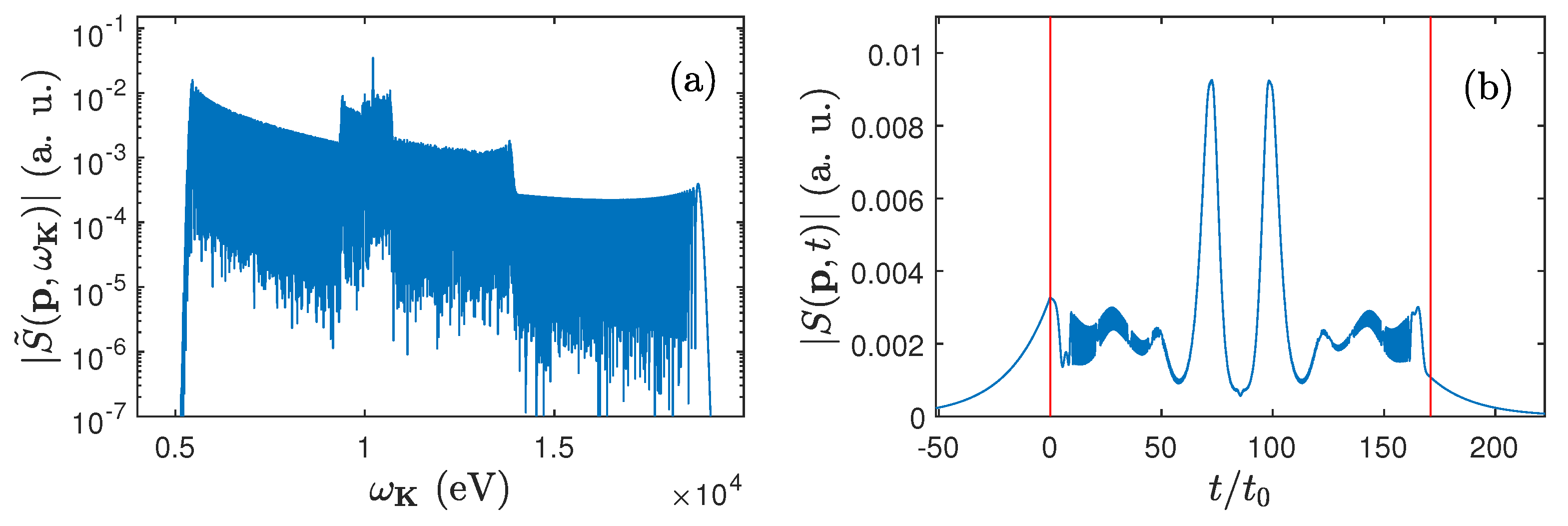
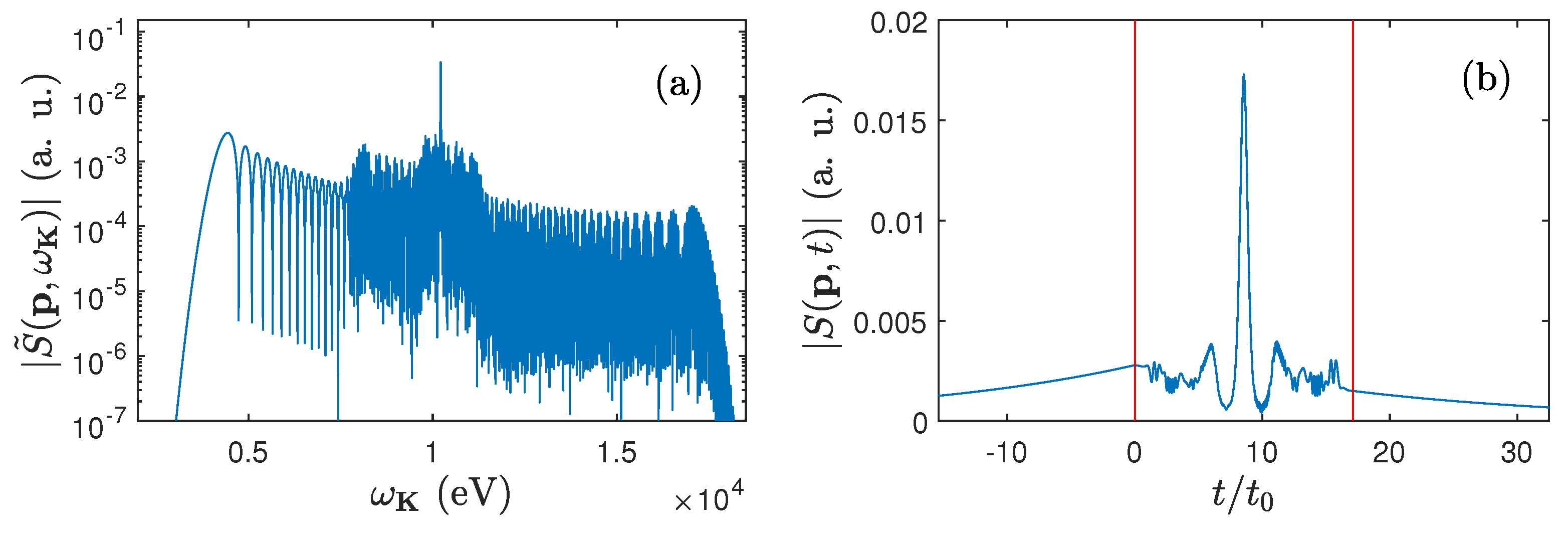
3.1. Energy Distributions of LARR Radiation

In Figure 2, we present the energy distributions of generated radiation in the case in which the aforementioned bicircular laser pulse accompanies the recombination of an electron wave packet (24) with the central energy $E_{\mathit{p}}={\mathit{p}}^2/2m_{\mathrm{e}}=10$ keV and the longitudinal momentum spread characterized by the parameter $\Delta \left|\mathit{p}\right|={10}^{-4}\sqrt{2m_{\mathrm{e}}{E}_{\mathit{p}}}=2.74\times {10}^{-3}{p}_0$ with a hydrogen-like ion ($\mathcal{Z}=4$). As denoted in Figure 2, we consider various configurations. While in panels (a) and (c), the electron is propagating in the x-direction, in panels (b) and (d) it is propagating in the opposite direction. Moreover, the generated radiation is linearly polarized either along the x-axis (panels (a), (b)) or along the y-axis (panels (c), (d)). In either case, it is emitted along the propagation direction of the laser pulse, ${\mathit{n}}_{\mathit{K}}={\mathit{e}}_z$. As one can see, all spectra consist of multiple plateaux spanning roughly the region of 10 keV photon energy. However, the spectra presented in panels (a) and (b) are by approximately two orders of magnitude more pronounced than those presented in panels (c) and (d). Also, in this more pronounced configurations, we observe a sharp peak at energy just above 10 keV. This peak originates from the laser-field-free process, resulting in the emitted radiation with energy ${\omega }_{\mathit{K}}$ (Equation (22)). As already elaborated in Ref. [6], the peak is absent when ${\mathit{\epsilon }}_{\mathit{K}}·\mathit{p}=0$, which is the case considered in panels (c) and (d). All energy spectra can be confronted with panels (e) and (f). The bottom panels of Figure 2 represent the prediction for an energy emitted by an electron of momentum $\mathit{p}$ that evolves in a laser pulse and is captured at time t by the ion. As it has been derived in Ref. [6], this energy in the leading nondipole order equals

$${\omega }_{\mathit{K}}\left(t\right)={\displaystyle \frac{1}{2m_{\mathrm{e}}}}{[\mathit{p}-e\mathit{A}\left(t\right)]}^2-E_B-{\displaystyle \frac{\mathit{n}·\mathit{p}}{m_e^{2}c}}\left[e\mathit{A}\left(t\right)·\mathit{p}-{\displaystyle \frac{1}{2}}{e}^2{\mathit{A}}^2\left(t\right)\right].$$

(40)

Note that the energy range of Equation (40), which is plotted in panels (e) and (f), matches the energy bandwidth of emitted LARR radiation presented in panels (a)–(d). The spectra exhibit also pronounced oscillations, which can be interpreted as arising from interference between different transition pathways [6,23]. One can realize from Equation (40) and from Figure 2e,f that the certain photon energy can be emitted at various times, each of them representing a given transition pathway. As the number of interfering pathways increases, additional plateaux are formed, with even more abrupt oscillations. The latter are not resolved on the scale of the figure though.

In Figure 3, we present the color mappings of the energy distributions of generated photons near the high-energy cutoff as a function of the recombining electron polar angle, ${\theta }_{\mathit{p}}$. The angle is measured with respect to the propagation direction of the laser pulse. Note that panel (a) represents the energy distribution of a radiation polarized linearly along the x-axis, whereas the same for polarization along the y-axis is shown in panel (b). The remaining parameters are the same as in Figure 2, except that now the incident direction of the electron is not fixed. One can realize that, in both presented cases, the maximum photon energy is generated for the electron polar angle smaller than $\pi /2$. This agrees nicely with Equation (40). As one can see from this formula, for as long as the accompanying pulse is treated in the dipole approximation, the photon energy distribution depends on $sin{\theta }_{\mathit{p}}$, so it is symmetric with respect to ${\theta }_{\mathit{p}}=\pi /2$. It is the inclusion of the nondipole corrections, which leads to asymmetry in the energy distributions presented in Figure 3. As the electron acquires a momentum from the laser pulse, it appears at a smaller incident polar angle ${\theta }_{\mathit{p}}$. As a result, the entire distribution is shifted toward smaller values of ${\theta }_{\mathit{p}}$. In addition, one can see a tiny interference pattern characterizing each distribution. It corresponds to very fast oscillations of the directional energy spectra presented in Figure 2.

For a comparison, we present also Figure 4 with the energy distributions of emitted radiation in the case in which both carrier frequencies of the laser pulse (Equations (37) and (38)) are increased to ${\omega }_1=50$ eV and ${\omega }_2=70$ eV. Two striking differences between this figure and Figure 2 can be seen. First of all, the present spectra are decreased by nearly an order of magnitude. At the same time, they exhibit less dense oscillations. Note that the remaining features of those energy distributions are the same as those in Figure 2. Namely, because they are dictated by the behavior of ${\omega }_{\mathit{K}}\left(t\right)$ (Equation (40)), which is the same in both cases (see panels (e) and (f) in Figure 2 and Figure 4). Nevertheless, one can conclude that the spectrum of the LARR radiation can be significantly suppressed (enhanced) depending on the bicircular laser field parameters.

The energy spectra presented in this section exhibit characteristic plateau regions. Hence, the question arises about temporal properties of the emitted LARR radiation. This is particularly interesting in the context of attosecond pulse generation, so it will be analyzed next.

3.2. Synthesis of Attosecond Pulses

We define the spectral distribution of emitted radiation (given in atomic units) as being proportional to the averaged probability amplitude of LARR, i.e., Equation (28):

$$\tilde{S}(\mathit{p},{\omega }_{\mathit{K}})={\mathcal{Z}}^{3/2}\sqrt{{\omega }_{\mathit{K}}}{\mathrm{e}}^{\pi \nu /2}\Gamma (1-\mathrm{i}\nu )\langle \mathcal{R}\left(\mathit{p}\right)\rangle .$$

(41)

Hence, the corresponding time distribution can be determined with the help of the Fourier transform such that

$$S(\mathit{p},t)=\int {\displaystyle \frac{\mathrm{d}{\omega }_{\mathit{K}}}{2\pi }}{\mathrm{e}}^{-\mathrm{i}{\omega }_{\mathit{K}}t}\tilde{S}(\mathit{p},{\omega }_{\mathit{K}}).$$

(42)

In addition, we define the window function $W\left({\omega }_{\mathit{K}}\right)$ that will allow us to filter a certain frequency bandwidth out of the LARR spectrum. The windowed spectral distribution is defined as

$${\tilde{S}}_W(\mathit{p},{\omega }_{\mathit{K}})=W\left({\omega }_{\mathit{K}}\right)\tilde{S}(\mathit{p},{\omega }_{\mathit{K}}),$$

(43)

and, similarly, its Fourier transform:

$$S_W(\mathit{p},t)=\int {\displaystyle \frac{\mathrm{d}{\omega }_{\mathit{K}}}{2\pi }}{\mathrm{e}}^{-\mathrm{i}{\omega }_{\mathit{K}}t}{\tilde{S}}_W(\mathit{p},{\omega }_{\mathit{K}}).$$

(44)

Essentially, the windowed distributions allow one to trace which portion of the energy spectrum of LARR radiation has a dominant contribution to the generated pulse. This will be demonstrated below.

In Figure 5a, we show the modulus of the spectral distribution of emitted radiation, defined by Equation (41), that corresponds to Figure 2a. The corresponding temporal distribution, Equation (42), is presented in Figure 5b. As one can see, it comprises of a main pulse centered around $80t_0$ and having FWHM duration of roughly $10t_0$. It is also accompanied by much weaker satellite pulses centered at approximately $60t_0$ and $110t_0$. The horizontal lines mark the time duration of the bicircular laser pulse. One can see that, essentially, the radiation is emitted in the presence of the laser field. There is also a nonzero signal outside of that time interval. This corresponds to laser-field-free recombination, discussed in Section 2. Next, in Figure 5c,e, we present the modulus of the windowed spectral distribution, Equation (43). We assume that the window function takes the following form:

$$W\left({\omega }_{\mathit{K}}\right)=\left\{\begin{array}{cc}1,\hfill & \mathrm{if}{\omega }_{\min }+\Delta \omega ⩽{\omega }_{\mathit{K}}⩽{\omega }_{\max }-\Delta \omega ,\hfill \\ {sin}^2\left({\displaystyle \frac{\pi }{2}}{\displaystyle \frac{{\omega }_{\mathit{K}}-{\omega }_{\min }}{\Delta \omega }}\right),\hfill & \mathrm{if}{\omega }_{\min }<{\omega }_{\mathit{K}}<{\omega }_{\min }+\Delta \omega ,\hfill \\ {sin}^2\left({\displaystyle \frac{\pi }{2}}{\displaystyle \frac{{\omega }_{\mathit{K}}-{\omega }_{\max }}{\Delta \omega }}\right),\hfill & \mathrm{if}{\omega }_{\max }-\Delta \omega <{\omega }_{\mathit{K}}<{\omega }_{\max },\hfill \\ 0,\hfill & \mathrm{otherwise},\hfill \end{array}\right.$$

(45)

where $\Delta \omega ={\eta }_W({\omega }_{\max }-{\omega }_{\min })$ and ${\eta }_W=0.1$. The remaining parameters are adjusted appropriately. Specifically, in order to plot Figure 5c, we have chosen ${\omega }_{\min }=11.5$ keV and ${\omega }_{\max }=18.5$ keV. In other words, we have selected a portion of the high-energy plateau from Figure 5a. Its low-energy plateau has been filtered out using ${\omega }_{\min }=2$ keV and ${\omega }_{\max }=7.9$ keV, and is shown in Figure 5e. Their respective temporal distributions, Equation (44), are shown in panels (d) and (f) of Figure 5, respectively. One can see from those panels that the high-energy radiation is generated in a form of two pulses, whereas the low-energy radiation is generated as an isolated pulse. The magnitudes of those pulses roughly correspond to the magnitudes of pulses recognized in panel (b). Therefore, the windowed distributions can be used to interpret the spectral properties of synthesized pulses. Specifically, in the given example, we conclude that it is the low-energy portion of the spectrum that contributes dominantly to the main pulse shown in Figure 5b.

In Figure 6, we present the modulus of the spectral distribution (panel (a)) and the modulus of the corresponding temporal distribution (panel (b)) of the radiation generated in Figure 2b. In other words, we consider now the case in which the electron wave packet is propagating in the opposite direction as compared to Figure 5. In contrast to Figure 5, we observe here two major pulses centered at approximately $70t_0$ and $100t_0$, each lasting for roughly $10t_0$ at FWHM. Even though we do not present here the numerical results, our analysis indicates that these pulses originate from the low-energy plateau region of Figure 6a. We note that this agrees with Figure 2f, representing an analytical estimate for the energy irradiated over time during the LARR process (Equation (40)). We understand that the radiation is most efficiently released at the crests where ${\omega }_{\mathit{K}}\left(t\right)$, given by Equation (40), takes the minimum value. This also indicates that, by appropriately tailoring the assisting laser pulse and adjusting the geometry of the process, we can, in principle, produce an arbitrary train of pulses.

In both examples studied so far, we have demonstrated a generation of attosecond bursts of radiation, lasting for roughly 200 as. This duration, however, can be significantly reduced, as we demonstrate next. In Figure 7a, we plot $|\tilde{S}(\mathit{p},{\omega }_{\mathit{K}})|$ for the case in which a bicircular laser field consists of two pulses, with the carrier frequencies ${\omega }_1=50$ eV and ${\omega }_2=70$ eV. More precisely, the presented spectral distributions correspond to Figure 4a. Note that the temporal distribution of generated radiation [panel (b)] shows a central pulse that has an FWHM duration of roughly 20 as. In other words, by increasing the carrier frequencies of the accompanying bicircular field by 10 times, we were able to decrease the radiated burst duration by 10 times as well. This means that the accompanying laser field plays a crucial role in controlling the properties of generated attosecond pulses in the LARR process.

4. Conclusions

We have studied the radiative recombination in the presence of a bicircular laser field using the recently developed theory [6], thus accounting for the Coulomb interaction and the nondipole corrections. Similar to the previously studied case of a linearly polarized laser pulse [6], we have observed multiple plateaux and a laser-field-free peak in the energy distributions of generated radiation. Those spectra show very abrupt oscillatory patterns which can be controlled by the parameters of the laser field, such as its two carrier frequencies. We have shown that variations of carrier frequencies of a bicircular laser field allow one to control the efficiency of produced radiation. Specifically, for the parameters used in the paper, we have observed nearly an order of magnitude enhancement of the LARR signal for smaller carrier frequencies.

As we have demonstrated, for the current parameters, the LARR radiation is released in a form of attosecond pulses. To illustrate this, we have investigated the spectral distributions of emitted radiation as well as their respective temporal distributions. As an interpretive tool, we have used the windowed distributions. We have observed both the generation of an isolated attosecond pulse and a train of two such pulses. As we have shown, the given outcome depends on the geometry of the process, and it can be manipulated by the external laser field. Had we tailored a laser pulse differently, we would be able to produce a train consisting of multiple attosecond pulses. It turned out that the properties of attosecond pulses themselves can be manipulated by the bicircular laser field. Specifically, we have shown that, by increasing the laser pulse carrier frequencies, one can significantly reduce the time duration of an isolated attosecond pulse. Thus, the engineering of laser fields with well-controlled properties is crucial for further investigations of LARR as a secondary source of radiation.

References

1. Nobel Prize in Physics 2023. Available online: https://www.nobelprize.org/prizes/physics/2023/summary/ (accessed on 17 February 2025).
2. Smeenk, C.T.L.; Arissian, L.; Zhou, B.; Mysyrowicz, A.; Villeneuve, D.M.; Staudte, A.; Corkum, P.B. Partitioning of the Linear Photon Momentum in Multiphoton Ionization. Phys. Rev. Lett. 2011, 106, 193002. [Google Scholar] [CrossRef] [PubMed]
3. Ludwig, A.; Maurer, J.; Mayer, B.W.; Phillips, C.R.; Gallmann, L.; Keller, U. Breakdown of the Dipole Approximation in Strong-Field Ionization. Phys. Rev. Lett. 2014, 113, 243001. [Google Scholar] [PubMed]
4. Wang, M.-X.; Chen, S.-G.; Liang, H.; Peng, L.-Y. Review on non-dipole effects in ionization and harmonic generation of atoms and molecules. Chin. Phys. B 2020, 29, 013302. [Google Scholar]
5. Maurer, J.; Keller, U. Ionization in intense laser fields beyond the electric dipole approximation: Concepts, methods, achievements and future directions. J. Phys. B At. Mol. Opt. Phys. 2021, 54, 094001. [Google Scholar]
6. Kanti, D.; Majczak, M.M.; Kamiński, J.Z.; Peng, L.-Y.; Krajewska, K. Laser-assisted radiative recombination beyond the dipole approximation. Phys. Rev. A 2024, 110, 043112. [Google Scholar]
7. Jaroń, A.; Kamiński, J.Z.; Ehlotzky, F. Stimulated radiative recombination and X-ray generation. Phys. Rev. A 2000, 61, 023404. [Google Scholar]
8. Kuchiev, M.Y.; Ostrovsky, V.N. Multiphoton radiative recombination of electron assisted by a laser field. Phys. Rev. A 2000, 61, 033414. [Google Scholar]
9. Jaroń, A.; Kamiński, J.Z.; Ehlotzky, F. Bohr’s correspondence principle and x-ray generation by laser-stimulated electron-ion recombination. Phys. Rev. A. 2001, 63, 055401. [Google Scholar]
10. Milošević, D.B.; Ehlotzky, F. Rescattering effects in soft-X-ray generation by laser-assisted electron-ion recombination. Phys. Rev. A 2002, 65, 042504. [Google Scholar]
11. Bivona, S.; Bonanno, G.; Burlon, R.; Leone, C. Polarization and angular distribution of the radiation emitted in laser-assisted recombination. Phys. Rev. A 2007, 76, 031402. [Google Scholar]
12. Zheltukhin, A.N.; Flegel, A.V.; Frolov, M.V.; Manakov, N.L.; Starace, A.F. Resonant phenomena in laser-assisted radiative attachment or recombination. J. Phys. B At. Mol. Opt. Phys. 2012, 45, 081001. [Google Scholar] [CrossRef]
13. Jaroń, A.; Kamiński, J.Z.; Ehlotzky, F. Coherent phase control in laser-assisted radiative recombination and X-ray generation. J. Phys. B At. Mol. Opt. Phys. 2001, 34, 1221–1232. [Google Scholar] [CrossRef]
14. Bivona, S.; Burlon, R.; Ferrante, G.; Leone, C. Control of multiphoton radiative recombination through the action of two low-frequency fields. Laser Phys. Lett. 2004, 1, 118–123. [Google Scholar]
15. Odžak, S.; Milošević, D.B. Bicircular-laser-field-assisted electron-ion radiative recombination. Phys. Rev. A 2015, 92, 053416. [Google Scholar] [CrossRef]
16. Čerkić, A.; Busuladžić, M.; Milošević, D.B. Electron-ion radiative recombination assisted by a bichromatic elliptically polarized laser field. Phys. Rev. A 2017, 95, 063401. [Google Scholar]
17. Tutmić, A.; Čerkić, A.; Busuladžić, M.; Milošević, D.B. Role of the relative phase and intensity ratio in electron-ion recombination assisted by a bicircular laser field. Eur. Phys. J. D 2019, 73, 231. [Google Scholar] [CrossRef]
18. Hu, S.X.; Collins, L.A. Intense laser-induced recombination: The inverse above-threshold ionization process. Phys. Rev. A 2004, 70, 013407. [Google Scholar] [CrossRef]
19. Kamiński, J.Z.; Ehlotzky, F. Time-frequency analysis of X-ray generation by recombination in short laser pulses. Phys. Rev. A 2005, 71, 043402. [Google Scholar] [CrossRef]
20. Bivona, S.; Burlon, R.; Ferrante, G.; Leone, C. Radiative recombination in the presence of a few cycle laser pulse. Opt. Express 2006, 14, 3715–3723. [Google Scholar]
21. Bivona, S.; Burlon, R.; Leone, C. Controlling laser assisted radiative recombination with few-cycle laser pulses. Laser Phys. Lett. 2007, 4, 44–49. [Google Scholar]
22. Čerkić, A.; Milošević, D.B. Few-cycle-laser-pulse-assisted electron-ion radiative recombination. Phys. Rev. A 2013, 88, 023414. [Google Scholar]
23. Kanti, D.; Kamiński, J.Z.; Peng, L.-Y.; Krajewska, K. Laser-assisted electron-atom radiative recombination in short laser pulses. Phys. Rev. A 2021, 104, 033112. [Google Scholar] [CrossRef]
24. Eichmann, H.; Egbert, A.; Nolte, S.; Momma, C.; Wellegehausen, B.; Becker, W.; Long, S.; McIver, J.K. Polarization-dependent high-order two-color mixing. Phys. Rev. A 1995, 51, R3414–R3417. [Google Scholar] [CrossRef] [PubMed]
25. Milošević, D.B.; Becker, W.; Kopold, R. Generation of circularly polarized high-order harmonics by two-color coplanar field mixing. Phys. Rev. A 2000, 61, 063403. [Google Scholar] [CrossRef]
26. Fleischer, A.; Kfir, O.; Diskin, T.; Sidorenko, P.; Cohen, O. Spin angular momentum and tunable polarization in high-harmonic generation. Nat. Photon. 2014, 8, 543–549. [Google Scholar] [CrossRef]
27. Medišauskas, L.; Wragg, J.; van der Hart, H.; Ivanov, M.Y. Generating Isolated Elliptically Polarized Attosecond Pulses using Bichromatic Counterrotating Circularly Polarized Laser Fields. Phys. Rev. Lett. 2015, 115, 153001. [Google Scholar]
28. Fan, T.; Grychtol, P.; Knut, R.; Hernández-García, C.; Hickstein, D.D.; Zusin, D.; Gentry, C.; Dollar, F.J.; Mancuso, C.A.; Hogle, C.W.; et al. Bright circularly polarized soft X-ray high harmonics for X-ray magnetic circular dichroism. Proc. Natl. Acad. Sci. USA 2015, 112, 14206–14211. [Google Scholar]
29. Baykusheva, D.; Ahsan, M.S.; Lin, N.; Wörner, H.J. Bicircular High-Harmonic Spectroscopy Reveals Dynamical Symmetries of Atoms and Molecules. Phys. Rev. Lett. 2016, 116, 123001. [Google Scholar]
30. Frolov, M.V.; Manakov, N.L.; Minina, A.A.; Vvedenskii, N.V.; Silaev, A.A.; Ivanov, M.Y.; Starace, A.F. Control of Harmonic Generation by the Time Delay Between Two-Color, Bicircular Few-Cycle Mid-IR Laser Pulses. Phys. Rev. Lett. 2018, 120, 263203. [Google Scholar] [CrossRef]
31. Berestetskii, V.B.; Lifshitz, E.M.; Pitaevskii, L.P. Quantum Electrodynamics, 2nd ed.; Pergamon Press: Oxford, UK, 1982; pp. 137–140. [Google Scholar]
32. Newton, R.G. Scattering Theory of Waves and Particles, 2nd ed.; Springer: New York, NY, USA, 1982; pp. 424–427. [Google Scholar]
33. Allegre, H.; Broughton, J.J.; Klee, T.; Li, Y.; Kowalczyk, K.M.; Thatte, N.; Lim, D.; Marangos, J.P.; Matthews, M.M.; Tisc, J.W.G. Extension of high-harmonic generation cutoff in solids to 50 eV using MgO. Opt. Lett. 2025, 50, 1492–1495. [Google Scholar]
Figure 1. Parametric plots of the electric field [panel (a)] and the vector potential [panel (b)] representing a bicircular laser pulse characterized by the following parameters: ω 1 = 5 eV, A 01 = 7 p 0 / | e | , N osc , 1 = 5 , δ 1 = π / 4 , and ω 2 = 7 eV, A 02 = 7 p 0 / | e | , N osc , 2 = 7 , and δ 2 = π / 4 . The field is plotted for z = 0 , meaning that t R = t . Note that, for the case in which we increase the carrier frequencies to ω 1 = 50 eV and ω 2 = 70 eV, the magnitude of the electric field presented in panel (a) has to be multiplied by a factor of 10.
Photonics 12 00320 g001
Figure 2. Energy distributions of radiation (Equation (35)) that is emitted when an electron described by a Lorentzian wave packet (Equations (24) and (25)) with a central energy E p = 10 keV and the longitudinal momentum spread characterized by the parameter Δ | p | = 2.74 × 10 3 p 0 recombines with a hydrogen-like ion ( Z = 4 ) in a presence of a bicircular laser pulse. The latter consists of a pair of counter-rotating circularly polarized laser pulses, that propagate along the z-axis ( n = e z ) and are described by the parameters: ω 1 = 5 eV, A 01 = 7 p 0 / | e | , N osc , 1 = 5 , δ 1 = π / 4 , and ω 2 = 7 eV, A 02 = 7 p 0 / | e | , N osc , 2 = 7 , δ 2 = π / 4 (Equations (37) and (38)). We assume that the LARR radiation is emitted in the z-direction ( n K = e z ) while being linearly polarized either along the x-axis (panels (a,b)) or the y-axis (panels (c,d)). As indicated in the figure, the electron wave packet propagates in the x-direction (panels (a,c)) or opposite to it (panels (b,d)). The corresponding energy irradiated at time t, ω K ( t ) , is plotted in panels (e,f) according to Equation (40).
Photonics 12 00320 g002
Figure 3. Color mappings of the energy distributions of emitted LARR radiation (Equation (35)) near the high-energy cutoff at varied polar angle of the recombining electron θ p . The parameters are the same as those in Figure 2. While panel (a) corresponds to the geometry of Figure 2a, panel (b) corresponds to the geometry of Figure 2c. The presented distributions are asymmetric with respect to θ p = π / 2 , which is attributed to nondipole effects.
Photonics 12 00320 g003
Figure 4. The same as in Figure 2 but for the carrier frequencies of the bicircular laser field ω 1 = 50 eV and ω 2 = 70 eV.
Photonics 12 00320 g004
Figure 5. Panel (a) shows the modulus of the spectral distribution of the radiation (41) considered in Figure 2a. The modulus of its corresponding temporal distribution (42) is presented in panel (b). Here, the vertical lines mark the turn on and off of the bicircular laser pulse assisting the process. The window-selected spectral distributions from the high-energy and the low-energy plateaux presented in panel (a) are shown in panels (c) and (e), respectively. They are synthesized to either a train of two pulses or an isolated pulse, as represented in panels (d,f).
Photonics 12 00320 g005
Figure 6. Modulus of the spectral distribution of the LARR radiation (41) shown in Figure 4a (panel (a)). The radiation is emitted as a train of two pulses, as seen in panel (b). The vertical lines mark the time duration of the bicircular laser field assisting the process.
Photonics 12 00320 g006
Figure 7. The same as in Figure 6 but for the case considered in Figure 4a.
Photonics 12 00320 g007
Disclaimer/Publisher’s Note: The statements, opinions and data contained in all publications are solely those of the individual author(s) and contributor(s) and not of MDPI and/or the editor(s). MDPI and/or the editor(s) disclaim responsibility for any injury to people or property resulting from any ideas, methods, instructions or products referred to in the content.