Incoherent Optical Neural Networks for Passive and Delay-Free Inference in Natural Light

Abstract

Optical neural networks are hardware neural networks implemented based on physical optics, and they have demonstrated advantages of high speed, low energy consumption, and resistance to electromagnetic interference in the field of image processing. However, most previous optical neural networks were designed for coherent light inputs, which required the introduction of an electro-optical conversion module before the optical computing device. This significantly hindered the inherent speed and energy efficiency advantages of optical computing. In this paper, we propose a diffraction algorithm for incoherent light based on mutual intensity propagation, and on this basis, we established a model of an incoherent optical neural network. This model is completely passive and directly performs inference calculations on natural light, with the detector directly outputting the results, achieving target classification in an all-optical environment. The proposed model was tested on the MNIST, Fashion-MNIST, and ISDD datasets, achieving classification accuracies of 82.32%, 72.48%, and 93.05%, respectively, with experimental verification showing an accuracy error of less than 5%. This neural network can achieve passive and delay-free inference in a natural light environment, completing target classification and showing good application prospects in the field of remote sensing.

1. Introduction

Traditional remote sensing detection methods, particularly electronic computing-based image processing algorithms, face numerous challenges, including slow computation speed and high energy consumption when handling large-scale remote sensing data. These issues make it difficult to meet the demands for real-time performance and low power consumption. As remote sensing technology rapidly advances, the number of remote sensing platforms and sensors continues to increase and is constantly being optimized, leading to a rapid growth in the volume of massive multi-source remote sensing data [1,2,3]. Therefore, developing an efficient and low-energy image processing technology has become an important research direction in the field of remote sensing detection. In recent years, optical neural networks (ONNs), as hardware neural networks implemented based on physical laws, have shown great potential in the field of deep learning [4,5,6,7]. Compared with traditional electronic computing, optical neural networks have advantages such as high speed, low energy consumption, and resistance to electromagnetic interference, making them particularly suitable for handling large-scale parallel computing tasks. They have already achieved good development in fields such as computer vision [8,9,10,11,12,13,14,15,16,17,18,19,20], optical communication [21,22,23,24,25], and multimodal signal processing [26,27,28,29,30,31,32,33,34,35,36]. However, most existing optical neural networks are designed for coherent light inputs, which means that in practical applications, an electro-optical conversion module needs to be introduced before the optical computing device. This conversion not only increases the complexity of the system but also significantly hinders the inherent speed and energy efficiency advantages of optical computing, limiting the application of optical neural networks in actual target detection tasks.

To overcome this limitation, researchers have begun to explore the design methods of incoherent optical neural networks (ICONN). Incoherent optical neural networks aim to directly receive natural light input for inference calculations, avoiding the step of electro-optical conversion, thereby preserving the high speed and low energy consumption characteristics of optical computing [37]. M. Kleiner et al. discussed how the performance of diffractive neural networks is affected by the coherence length and coherence time of the light source, and they proposed optimization schemes for network design with incoherent light inputs [38]. M.S.S. Rahman et al. studied the use of spatially incoherent diffractive processors to achieve universal linear intensity transformations, demonstrating the application potential of incoherent optical neural networks in fields such as imaging and signal processing [39]. In the same year, the team also investigated the use of diffractive optical neural networks for signal restoration in the presence of arbitrary opaque occlusions, showing the application of robust optical communication systems in complex environments [40]. B. Rahmani et al. proposed a method for transmitting full-optical images through multimode fibers using incoherent light, employing diffractive optical neural networks to compensate for distortions caused by multimode fibers, indicating the feasibility of using incoherent light in diffractive neural-network-based optical communication and imaging systems [7]. The method proposed by S. Sun’s team, based on partially coherent optical neural networks (PCONN), although theoretically promising, is limited in practical applications due to the complexity of coherence measurements, which restricts its performance [41]. The incoherent all-optical methods mentioned above still have defects such as difficulty in training, large simulation errors, and the need for electrical domain activation.

In response to the aforementioned issues, this paper proposes a diffractive algorithm for incoherent light based on mutual intensity propagation [42,43,44] and establishes a model of an incoherent optical neural network on this basis. The model is completely passive, directly performing inference calculations on natural light, and it does not require any electro-optical conversion modules before outputting the light intensity at the detection surface, thereby achieving target classification in an all-optical environment. The main contributions of this paper include (1) proposing a new diffractive algorithm for incoherent light that can effectively handle natural light inputs; (2) establishing an incoherent optical neural network model based on this algorithm, achieving passive inference, and conducting simulation tests on the MNIST, Fashion-MNIST, and ISDD datasets, achieving accuracies of 82.32%, 72.48%, and 93.05%, respectively, and analyzing various factors that may affect the model’s performance; (3) setting up an optical platform to experimentally verify the proposed model, with an error in simulation accuracy of less than 5%, proving the model’s effectiveness and robustness in a natural light environment.

The method proposed in this paper still has room for further development. First, the model has currently only been tested and verified on image classification datasets, and in the future, it can be further tested and optimized for object detection tasks on large-scale remote sensing datasets. Second, because the model directly receives natural light input, it is difficult for the network to generate nonlinear activation, which limits the network’s performance on complex tasks. Possible solutions include exploring weak-light nonlinear mechanisms for natural light or introducing a small amount of electrical domain computation to provide nonlinearity. Future research will focus on solving these problems to further enhance the performance of incoherent optical neural networks in practical applications.

2. Methods

2.1. Subsection

There are two commonly used analytical algorithms for the diffractive transmission of incoherent light. One is based on Fourier optics, which calculates the output through spectral conversion [37,45,46]. This method is usually suitable for simple imaging systems; otherwise, the propagation modes of different spectral components will vary, causing the system to be space-variant and resulting in errors. The other is the random phase superposition method based on statistics [39,47]. This method interprets the input of incoherent light fields as the superposition of multiple coherent lights with random initial phases. These coherent lights are transmitted independently, and then the field strength is calculated separately at the output surface before performing an incoherent average. To obtain a stable output, this method typically requires a high number of superimposed layers, resulting in high computational power demand. Moreover, both of the above algorithms require the input to be completely incoherent light for calculation. In other words, when there are changes in coherence within the system, they cannot perform segmented optimization. In practical applications, especially in the field of remote sensing, long-distance transmission often causes the coherence of the light field to change in various ways. In this paper, we adopted a transmission theory for incoherent light fields based on mutual intensity propagation. This method does not rely on statistical laws, which reduces the computational power demand to a certain extent. Moreover, since the coherence of the light field is fully preserved, the calculation can start at any point in the system. Therefore, the system can be modeled in segments, corresponding to the multi-layer network in neural network algorithms, allowing for layer-by-layer optimization. The following is the derivation of this transmission model.

In nature, targets can be regarded as incoherent light at the initial plane, that is, the degree of partial coherence is 0. Therefore, the input light field can be established as

$$\mathrm{J}({\mathrm{P}}_1,{\mathrm{P}}_2)=\mathrm{I}({\mathrm{P}}_1)\mathsf{\delta }({\mathrm{P}}_1-{\mathrm{P}}_2)$$

(1)

In Equation (1), J represents the mutual intensity, I represents the light field intensity, P₁ and P₂ represent the initial plane of the light field emitted by the target, and the delta function indicates that the value of J is equal to I only when P₁ and P₂ overlap. When P₁ and P₂ do not overlap, J = 0, indicating complete incoherence.

The general propagation formula for partial coherence can be obtained from the statistical law of Rayleigh Sommerfeld diffraction formula, that is,

$$\begin{array}{c}\mathrm{J}({\mathrm{Q}}_1,{\mathrm{Q}}_2)=〈\mathrm{u}*({\mathrm{Q}}_1)\mathrm{u}({\mathrm{Q}}_2)〉\hfill \\ ={\displaystyle \frac{1}{4{\mathsf{\pi }}^2}}{\displaystyle \iint {\displaystyle \iint \mathrm{J}({\mathrm{P}}_1,{\mathrm{P}}_2)}\exp [\mathrm{j}\mathrm{k}({\mathrm{r}}_2-{\mathrm{r}}_1)]\frac{\mathrm{K}({\mathsf{\theta }}_1)}{{\mathrm{r}}_1}\frac{\mathrm{K}({\mathsf{\theta }}_2)}{{\mathrm{r}}_2}(\frac{1}{{\mathrm{r}}_1}+\mathrm{j}\mathrm{k})(\frac{1}{{\mathrm{r}}_2}-\mathrm{j}\mathrm{k})}\mathrm{d}{\mathrm{S}}_1\mathrm{d}{\mathrm{S}}_2\end{array}$$

(2)

In Equation (2), J(Q₁, Q₂) represents the distribution of mutual intensity at the output plane; r₁ and r₂ represent the distances between P₁, Q₁ and P₂, Q₂, respectively; and K(${\mathsf{\theta }}_1$) and K(${\mathsf{\theta }}_2$) represent the tilt factors in diffraction. The above equation represents the mapping relationship between the mutual intensity of two planes in free space, and there is no approximation, which follows the space-invariant principle. Therefore, it can be established as a convolution formula:

$$\begin{array}{c}\mathrm{J}({\mathrm{Q}}_1,{\mathrm{Q}}_2)={\displaystyle \iint \mathrm{J}({\mathrm{P}}_1,{\mathrm{P}}_2)}\mathrm{h}({\mathrm{P}}_1){\mathrm{h}}^{*}({\mathrm{P}}_2)\mathrm{d}{\mathrm{S}}_1\mathrm{d}{\mathrm{S}}_2\\ =\mathrm{J}({\mathrm{P}}_1,{\mathrm{P}}_2)\ast \mathrm{h}({\mathrm{P}}_1,{\mathrm{P}}_2,{\mathrm{Q}}_1,{\mathrm{Q}}_2)\end{array}$$

(3)

In Equation (3), h is the point spread function of mutual intensity in free space. Further solving the Fourier transform of this point spread function allows us to transfer Equation (2) to the frequency domain calculation, which means that we can greatly accelerate our calculation process using the fast Fourier transform (FFT) algorithm. As mentioned earlier, this method can perform segmented optimization on the network.

After the light field has been transmitted, we can process the light field characterized by partial coherence according to the system requirements to obtain the desired information. In our task, what we need is the intensity of the final detection plane. Assuming the output surface coordinates are Q′(x, y), it can be obtained by setting Q′₁ = Q′₂:

$$\mathrm{I}(\mathrm{Q}{\prime }_1)=\mathrm{J}(\mathrm{Q}{\prime }_1,\mathrm{Q}{\prime }_2){|}_{\mathrm{Q}{\prime }_1=\mathrm{Q}{\prime }_2}$$

(4)

In addition, we also note that in remote sensing scenarios, the targets are usually very far from the system, and this distance usually satisfies the Fresnel approximation. Then, we can derive the Van Cittert–Zernike theorem in partial coherent optics:

$$\mathrm{J}({\mathrm{x}}_1,{\mathrm{y}}_1;{\mathrm{x}}_2,{\mathrm{y}}_2)={\displaystyle \frac{\exp (\mathrm{j}\mathsf{\psi })}{{(\overline{\mathsf{\lambda }}\mathrm{z})}^2}}{\displaystyle \iint \mathrm{I}(\mathsf{\alpha },\mathsf{\beta })\exp \{-\mathrm{j}\frac{2\mathsf{\pi }}{\overline{\mathsf{\lambda }}\mathrm{z}}(\Delta \mathrm{x}\mathsf{\alpha }+\Delta \mathrm{y}\mathsf{\beta })\}\mathrm{d}\mathsf{\alpha }\mathrm{d}\mathsf{\beta }}$$

(5)

In Equation (5), α and β are the input surface coordinates, and x and y are the output surface coordinates. The meaning of this theorem is that when the size of the incoherent target itself and the observation plane are much smaller than the distance between them, the mutual intensity of the observation plane is only related to the relative distance between the two points. Specifically, the mutual intensity is proportional to the Fourier transform of the target intensity. This theorem is also important in our network, as it greatly simplifies the computational complexity of the input light field when mutual intensity is used as the propagation dimension, allowing us to directly establish the neural network model from the first acceptance plane of the system.

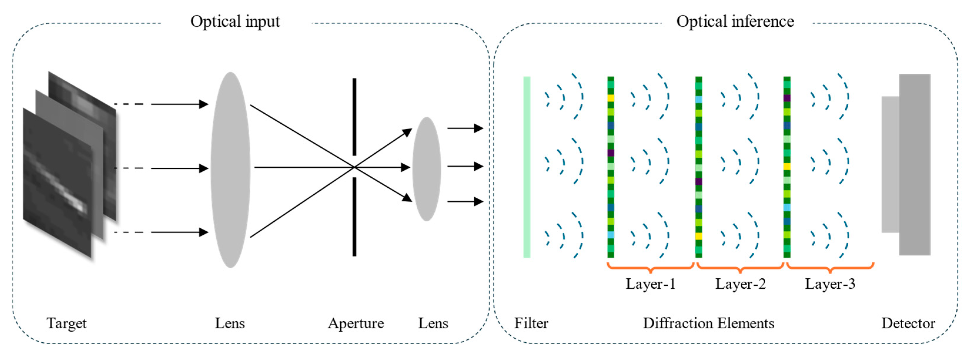
2.2. Principle of ICONN

The ICONN model designed in this paper is mainly divided into two modules: the optical input module and the optical inference module, as shown in Figure 1. In the left block diagram, the optical field input module is depicted, where the first lens serves as the system’s optical aperture, primarily used for imaging. According to the resolution requirements, an aperture is set on the imaging plane of this input module to filter out a specified small field of view. The small field of view is then transformed into partially coherent light by the second lens and output to the subsequent inference module. The main functions of this input module are light collection, image plane segmentation, and preserving the spatial coherence distribution of the light field.

The inference module mainly consists of multiple layers of incoherent optical neural networks. The optical neural network is composed of discrete diffractive devices. The spatial light field is modulated by the diffractive devices with linear phase modulation, and after diffracting a certain distance in free space, it is modulated again by the next layer of diffractive devices. After multiple layers of modulation and diffraction, the label distribution preset during the algorithm training phase can be obtained. The label is further measured by the output module. The modulation range of the diffractive devices is from 0 to 2π. During the training phase, the data type of the phase modulation quantity is set to float32, and it is re-quantified in the subsequent output manufacturing stage. We will discuss the impact of this quantization on network performance later in the text.

Here, we consider one modulation plus one free-space diffraction as one layer of the optical neural network. Therefore, a single-layer optical neural network can be modeled as

$${\mathrm{w}}_{\mathrm{i},\mathrm{j}}^{\mathrm{l}}({\mathrm{P}}_{\mathrm{i}},{\mathrm{P}}_{\mathrm{j}})={({\displaystyle \frac{{\mathrm{z}}_{\mathrm{l}}}{\overline{\mathsf{\lambda }}{\mathrm{r}}_{\mathrm{i}}{\mathrm{r}}_{\mathrm{j}}}})}^2\exp [{\displaystyle \frac{\mathrm{j}2\mathsf{\pi }({\mathrm{r}}_{\mathrm{j}}-{\mathrm{r}}_{\mathrm{i}})}{\overline{\mathsf{\lambda }}}}]$$

(6)

$${\mathrm{n}}_{\mathrm{i},\mathrm{j}}^{\mathrm{l}}({\mathrm{P}}_{\mathrm{i}},{\mathrm{P}}_{\mathrm{j}})={\mathrm{w}}_{\mathrm{i},\mathrm{j}}^{\mathrm{l}}({\mathrm{P}}_{\mathrm{i}},{\mathrm{P}}_{\mathrm{j}})\cdot {\mathrm{t}}_{\mathrm{i}}^{\mathrm{l}}(:,:,{\mathrm{x}}_{\mathrm{i}},{\mathrm{x}}_{\mathrm{i}})\cdot {\mathrm{t}}_{\mathrm{j}}^{{\mathrm{l}}^{*}}({\mathrm{x}}_{\mathrm{j}},{\mathrm{x}}_{\mathrm{j}},:,:)\cdot {\displaystyle \sum _{\mathrm{m},\mathrm{n}}{\mathrm{n}}_{\mathrm{m},\mathrm{n}}^{\mathrm{l}-1}({\mathrm{P}}_{\mathrm{m}},{\mathrm{P}}_{\mathrm{n}})}$$

(7)

In Equation (6), ${\mathrm{w}}_{\mathrm{i},\mathrm{j}}^{\mathrm{l}}({\mathrm{P}}_{\mathrm{i}},{\mathrm{P}}_{\mathrm{j}})$ represents the mutual intensity propagation mode of the four-dimensional sub-wave source $({\mathrm{P}}_{\mathrm{i}},{\mathrm{P}}_{\mathrm{j}})$, where l denotes the layer number in the network, and i and j represent a pair of points on the P-plane. ${\mathrm{z}}_{\mathrm{l}}$ is a constant representing the center distance between the l-th layer and the next layer. $\overline{\mathsf{\lambda }}$ represents the center wavelength of the optical field under the quasi-monochromatic approximation, and ${\mathrm{r}}_{\mathrm{i}}$ and ${\mathrm{r}}_{\mathrm{j}}$ represent the distances from the sub-wave source to the output point. In Equation (7), ${\mathrm{n}}_{\mathrm{i},\mathrm{j}}^{\mathrm{l}}({\mathrm{P}}_{\mathrm{i}},{\mathrm{P}}_{\mathrm{j}})$ represents the output function of the (i, j)-th neuron formed by $({\mathrm{P}}_{\mathrm{i}},{\mathrm{P}}_{\mathrm{j}})$ in the l-th layer of the network, where ${\mathrm{t}}_{\mathrm{i}}^{\mathrm{l}}$ denotes the mutual intensity modulation coefficient of the diffractive element.

There is a filter in front of the diffractive device, whose main function is to improve the temporal coherence of the light field and provide quasi-monochromatic light input for the modulation device. The final output result of the system is received by the detector, and the classification result is determined by the label area set during the training phase. The loss of the network is represented as

$$\mathrm{L}\mathrm{o}\mathrm{s}\mathrm{s}=\mathrm{M}\mathrm{S}\mathrm{E}({\mathrm{I}}_{\mathrm{g}\mathrm{t}}\cdot scale,\mathrm{I})$$

(8)

In Equation (8), we adopted the mean squared error (MSE) method to calculate our loss. I_gt represents the label distribution, and different classification tasks correspond to different label settings. I_real represents the network output result, and scale represents a scaling factor for the output. Since the output of the optical neural network usually does not perfectly match the label setting, appropriately scaling the label can help the network converge faster.

Optical neural networks typically have a small field of view, and our system also has this characteristic because we placed an aperture on the focal plane of the first lens to perform image plane filtering. However, we can achieve a larger field of view by arraying the system or through line scanning and area scanning methods. That is, our system can perform more complex tasks in a natural light environment, such as object detection, without the need for prior electro-optical conversion, followed by image cutting and using lasers and spatial light modulators to provide input for the subsequent inference model. Our method is expected to achieve real-time processing of massive remote sensing data.

3. Simulation and Experiment Results

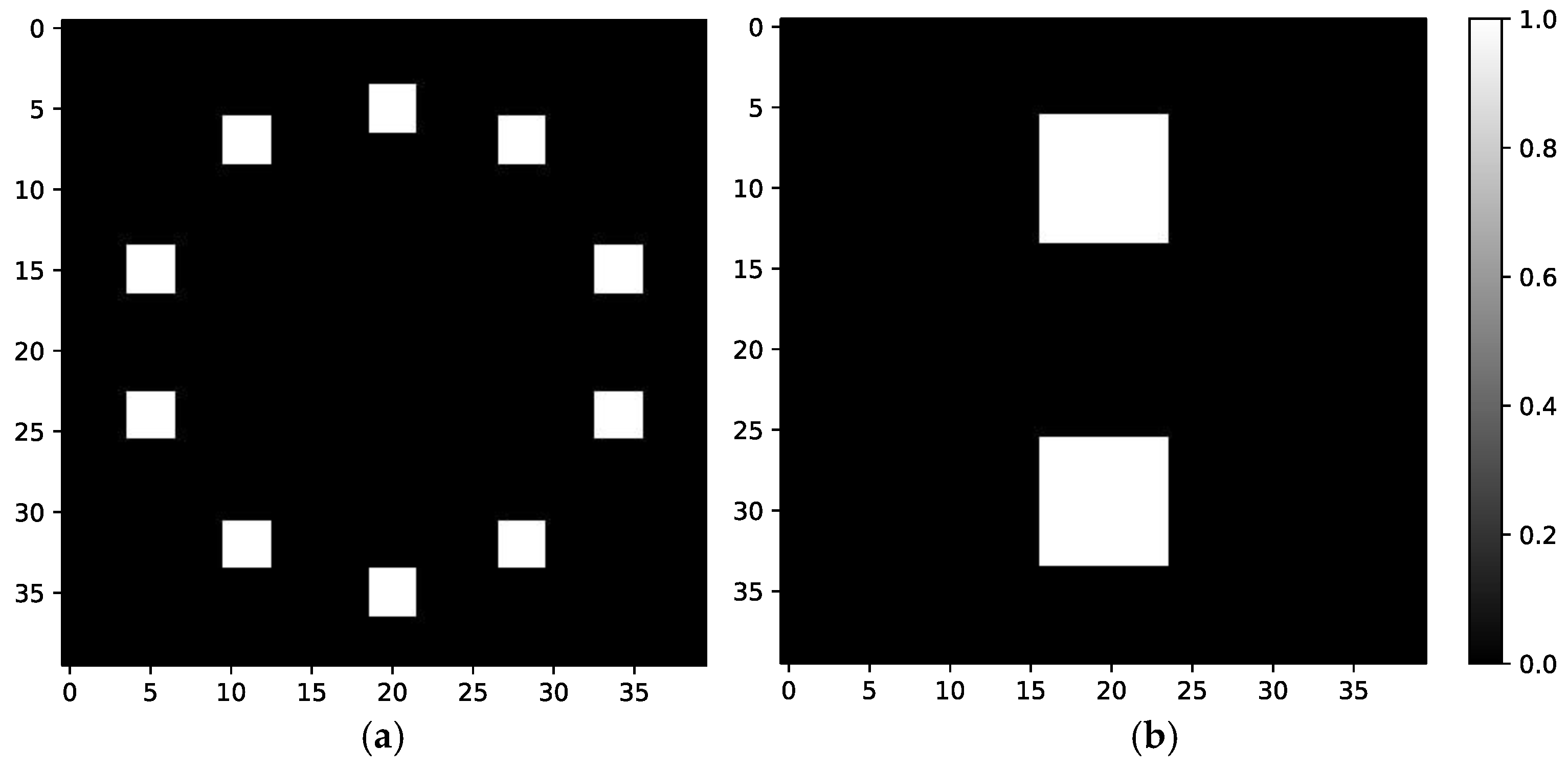
3.1. Simulation Strategy

The training and simulations were carried out in a CentOS 7.9.2009 environment, using an Nvidia@4090 graphics card and an AMD EPYC 7282 CPU. The simulation tests included performance evaluations of ICONNs with different numbers of layers, while the experimental tests focused on a single-layer ICONN. We will see in the following text that the simulation and experimental results for the single-layer case are in good agreement.

We conducted simulation tests on the ICONN model proposed earlier, with the detector ground truth settings shown in Figure 2. The ground truth is circularly distributed around the center of the effective detection area. The average light intensity within each square detection region corresponds to the score of a category, and the category with the highest average light intensity is the output category.

During the simulation and experimental testing phases, we used the general image classification datasets MNIST and Fashion MNIST, as well as an infrared ship detection dataset, ISDD, to evaluate the performance of the ICONN model. The first two image classification datasets are ten-class, corresponding to the ground truth in Figure 2a. For the ISDD dataset, we performed preprocessing to conduct binary classification, i.e., ship present and ship absent, corresponding to the ground truth in Figure 2b. The specific processing method is as follows: First, we read the labels (boxes) from the annotation files in the dataset and extracted fixed-width images centered on the label boxes as positive samples. Here, we set the width to 40 pixels, which has been verified to cover over 95% of the target bounding boxes. Then, we randomly generated images from the large image that do not overlap with the labeled bounding boxes and whose pixel grayscale values are not all less than 10 as negative samples. The ratio of positive to negative samples was approximately 1:1. The extracted small images were used as the new classification dataset for subsequent simulation and experimental testing. All datasets were divided into training and testing sets in a 4:1 ratio, with a batch size of 20. The loss function was the mean squared error (MSE) between the network output and the ground truth. The network operated entirely in the optical domain without the addition of activation functions, and the learning rate was set to 0.001.

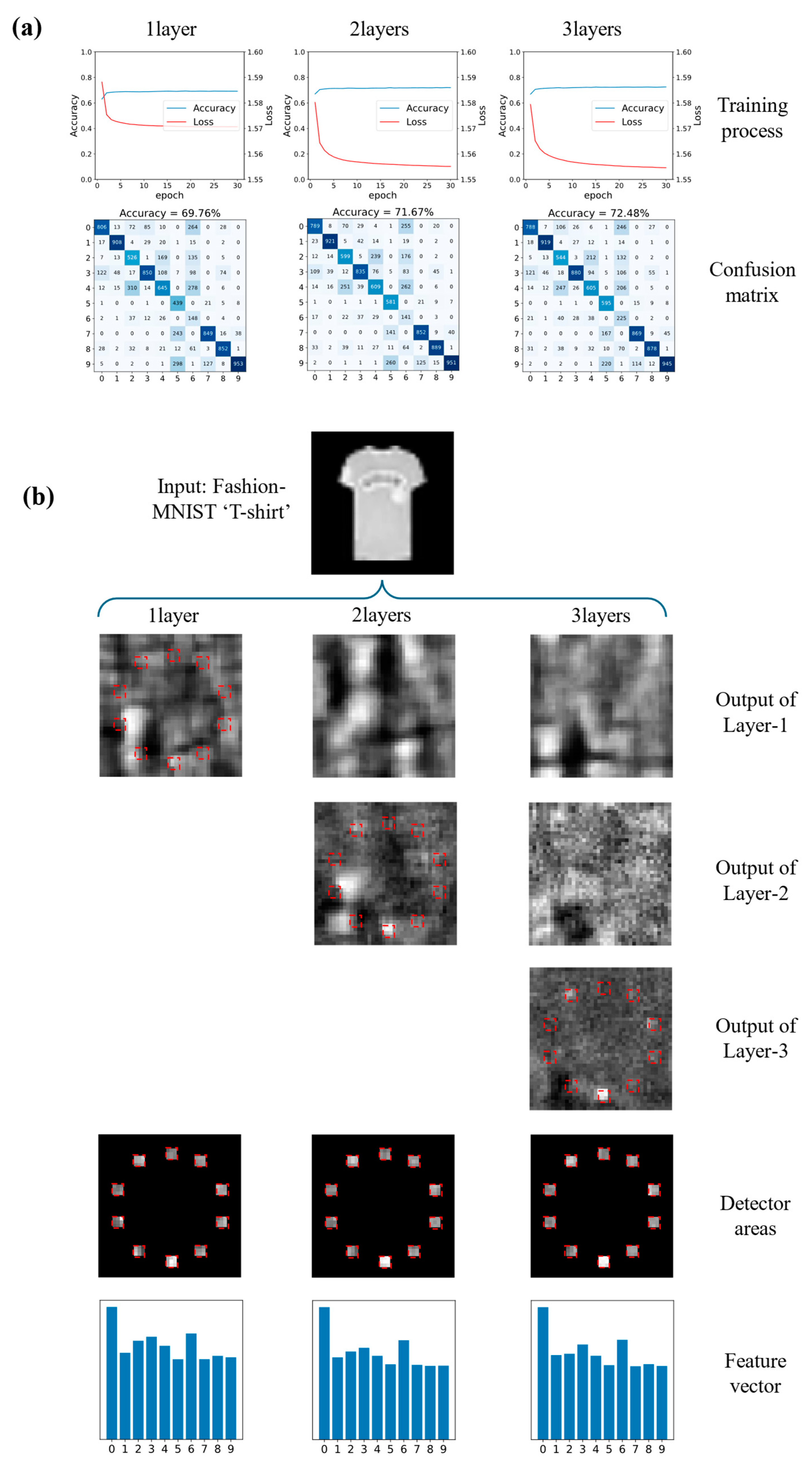
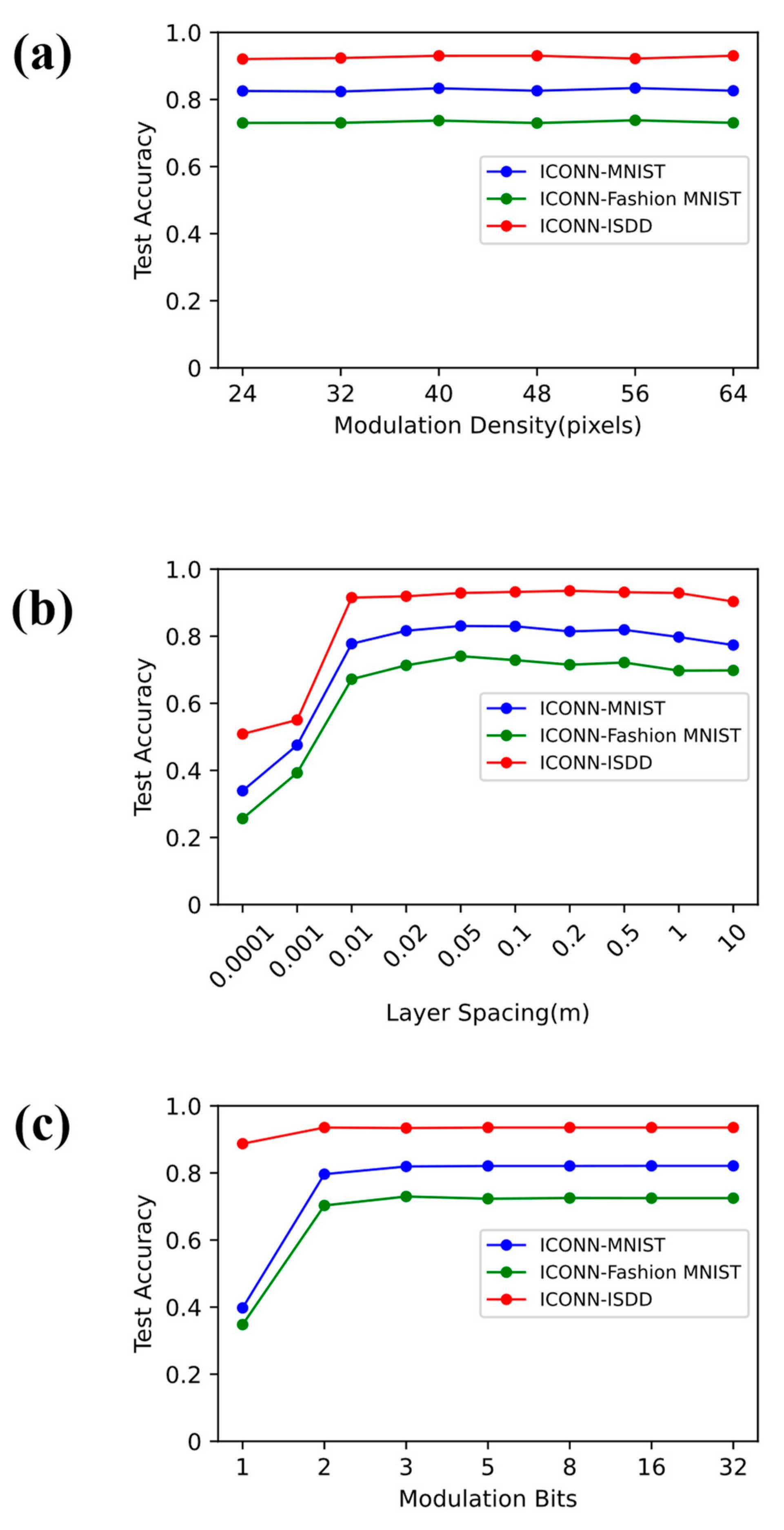
3.2. Simulation Result and Analysis

First, we conducted tests on the general image classification datasets MNIST and Fashion MNIST. The training was iterated for 30 epochs, and the performance of networks with 1 to 3 layers was tested. The simulation test accuracies were 79.75%, 82.11%, and 82.32% for MNIST, and 69.76%, 71.67%, and 72.48% for Fashion MNIST. The training results and inference demonstration are shown in Figure 3 and Figure 4. From the test results, we can observe that the performance of the ICONN network increased with the number of layers. However, since the ICONN network is a purely linear light intensity mapping, this increase is not significant compared to fully connected networks in the electrical domain or CONN/PCONN with one layer of nonlinear activation. Nevertheless, our simulation demonstration clearly shows that after increasing the number of layers, the label distribution on the detection surface was closer to the ideal ground truth. In other words, most of the energy was concentrated within the label boxes, and the proportion of light intensity for the correct label was higher. This can avoid misjudgments caused by insufficient detector sensitivity, noise, pixel alignment errors, etc., and is still helpful in practical detection tasks.

We also conducted tests on an open-source infrared remote sensing ship detection dataset. The network was trained for 30 epochs, and the performance of networks with 1 to 3 layers was tested. In line with the application characteristics of optical neural networks, we processed the remote sensing images based on the annotations in the dataset, with the processing method described in Section 3.1. The training parameters for the network were consistent with those in the previous section. The simulation test accuracies for networks with 1 to 3 layers were 92.15%, 92.89%, and 93.05%, respectively. The training results and inference demonstration are shown in Figure 5. Similar conclusions can be drawn from the test results: the performance of ICONN did not significantly improve with an increase in the number of layers, but the label distribution became more ideal and easier to measure. Moreover, the excellent performance of our model on the ISDD dataset demonstrated its great potential in the field of remote sensing detection.

In addition to the number of layers, we conducted simulation tests on other parameters that may affect the performance of ICONN, including modulation plane pixel density, layer spacing, and phase modulation bit depth. The modulation plane pixel density refers to the number of pixels contained in the modulation plane when the area of the modulation layer remains unchanged. This value can be adjusted by zero-padding the input image. The layer spacing refers to the diffraction distance of light in free space after passing through one layer of modulation. The phase modulation bit depth refers to the modulation precision of the modulation plane. In each of the above tests, the method of controlling variables was used, and the size of the input image and the size of the modulation layer remained unchanged. The results are shown in Figure 6.

The results show that for the three image classification datasets we tested, the original image resolution and the modulation device resolution had little impact on the network’s performance. However, the layer spacing, or more precisely, the Fresnel number F, which is related to the diffraction effect, had a significant impact on the network’s performance. The Fresnel number is defined as follows:

$$\mathrm{F}={\displaystyle \frac{{\mathrm{d}}^2}{\mathsf{\lambda }\mathrm{L}}}$$

(9)

In Equation (9), d represents the width of the diffraction plane, i.e., the modulation device, and L represents the diffraction distance, i.e., the layer spacing. When the area of our modulation device is fixed, if the layer spacing is set too small, the diffraction effect between layers is weak, and the light field propagation is more akin to geometric optics. The energy allocation effect brought by phase modulation is very weak, making it difficult for the model to converge. As the layer spacing increases and the diffraction between layers approaches Fresnel diffraction, the phase modulation can have a more pronounced energy allocation effect, making the output results more likely to converge to the preset label region. For this reason, in diffractive neural networks, increasing the pixel density of the modulation plane, or the number of neurons, has a limited impact on ICONN. This is because ICONN is driven by physical computation of diffraction effects, rather than the mathematically driven computation of electrical neural networks based on parameter scale. The physical propagation laws of light will somewhat limit the input–output mapping relationship. Our simulation results indicate that the network performance is optimal and stable when the Fresnel number is in the range of approximately 25 to 250. Generally, a shorter layer spacing can lead to a more compact and stable system. Therefore, it is sufficient to take the maximum value of the Fresnel number. This conclusion applies to optical neural networks based on diffraction effects.

The impact of phase modulation bit depth on network performance is also limited. Our network uses torch.complex64 type data during training, corresponding to a phase modulation precision of 24 bit. However, when we reduced the modulation precision to 3 bit during the testing phase, the network performance only dropped by about 1 percentage point. When reduced to 2 bit, the network performance dropped by 1–3 percentage points. Three bit means the network can only provide eight modulation phases: −3π/4, −π/2, −π/4, 0, π/4, π/2, 3π/4, π. Similarly, 2 bit can only provide four modulation phases: −π/2, 0, π/2, π. This demonstrates the remarkable robustness of ICONN to the modulation precision of modulation devices.

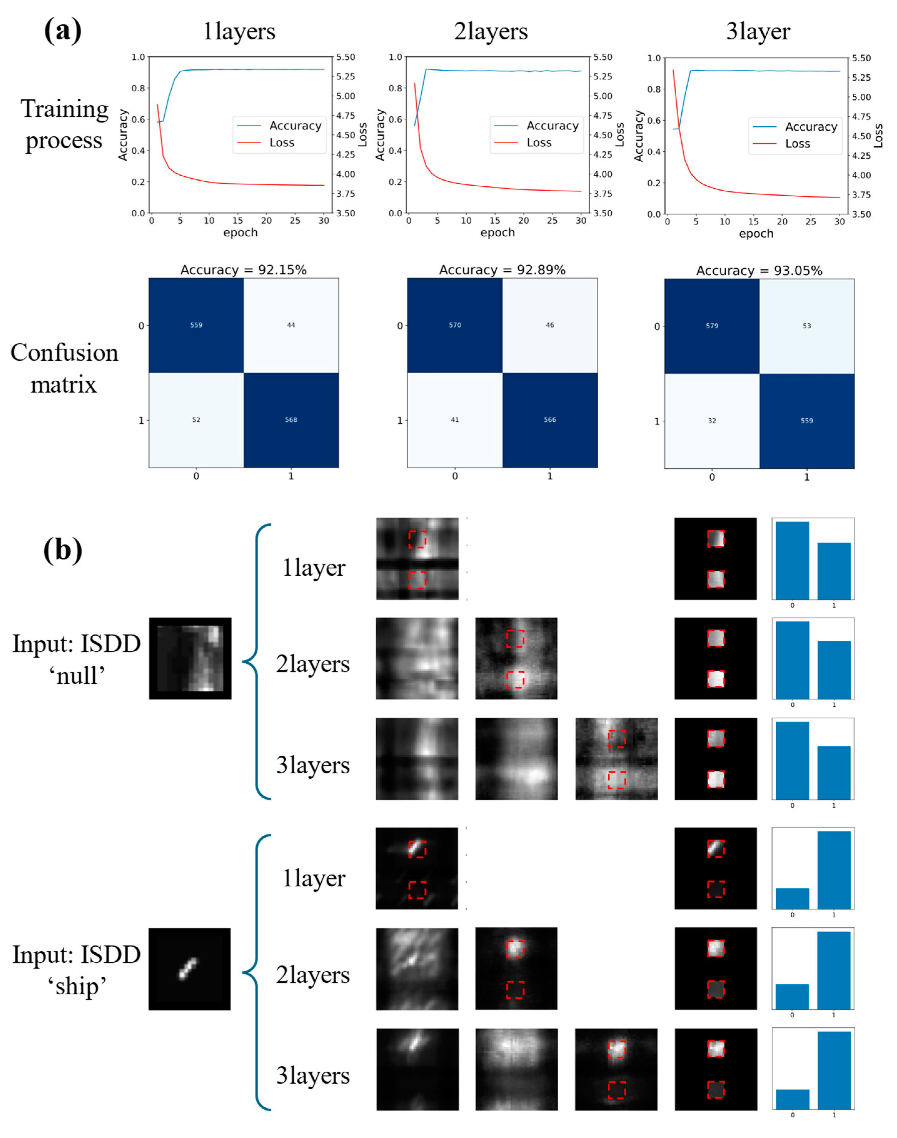
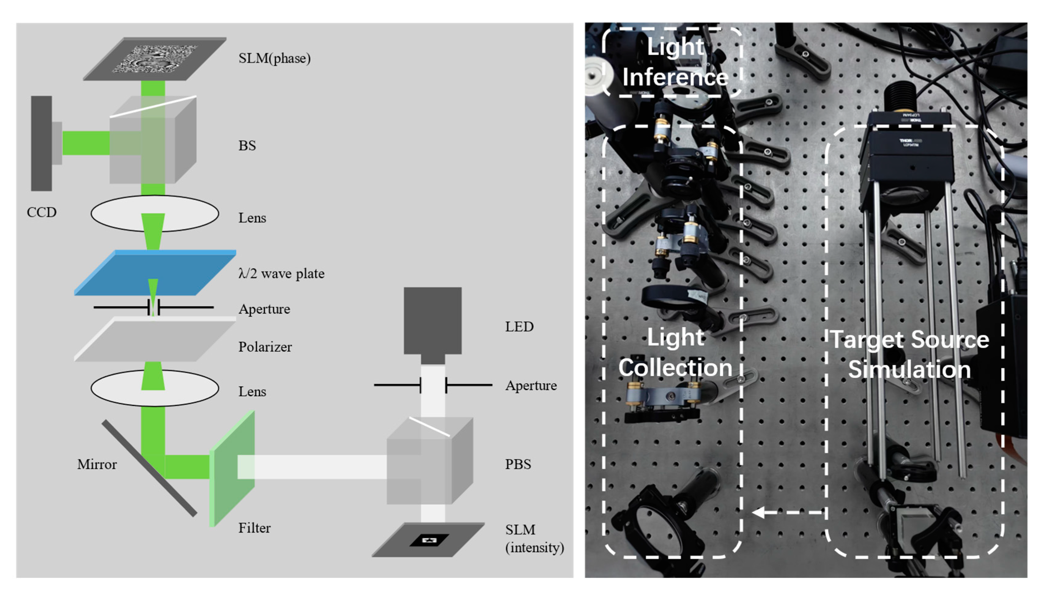
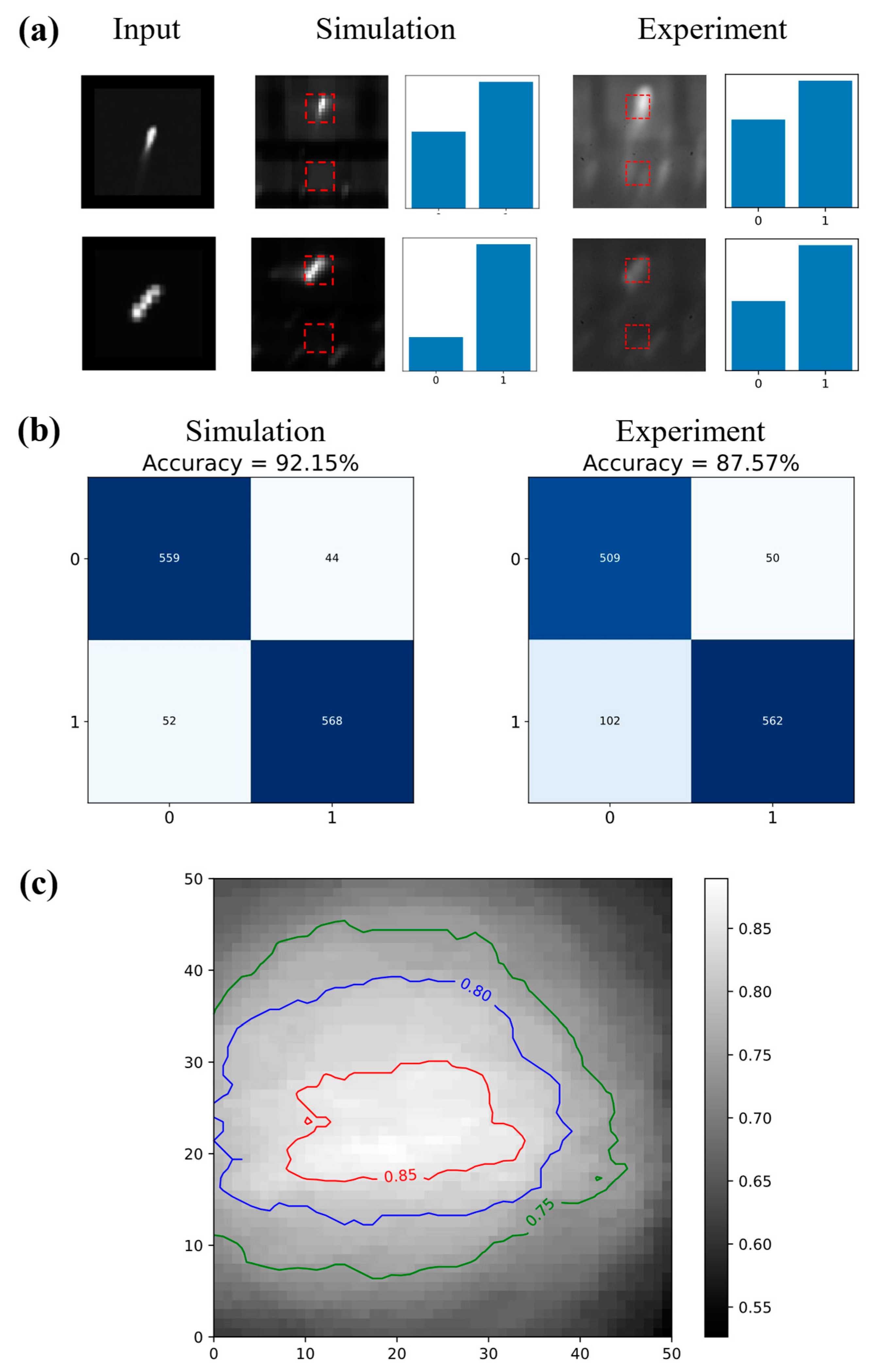
3.3. Experiment Result and Analysis

We constructed an ICONN experimental platform to verify our model, with the experimental optical layout depicted in Figure 7. The right side represents the optical input module, where we utilized a white light LED (MNWHL4, THORLABS), a polarized beam splitter, and an amplitude SLM (HDSLM80RA Plus, UPOlabs) loaded with the target intensity distribution to simulate incoherent light input from a natural environment. The left side comprises the optical inference module, which consists of a filter (532 nm ± 20 nm), a 4f system, a beam splitter, a polarizer, a phase SLM (PLUTO-2.1, HOLOEYE), and a CCD. The polarizer is employed to meet the polarization sensitivity requirements of the inference device, while the filter is used to obtain quasi-monochromatic light to satisfy the modeling needs. The 4f system is designed to cut the image plane and map the mutual intensity spectrum plane of the target onto the phase SLM. The phase SLM serves as the modulation layer in the neural network, modulating the input incoherent light field by loading the phase distribution trained in the electrical domain.

The input image had a pixel density of 80 × 80, with a pixel size of 32 μm. The modulation plane pixel density was set to 40 × 40. The distance from the target (amplitude SLM) to the front focal plane of the 4f system was set to 0.308 m, which satisfied the Fresnel approximation. According to the Van Cittert–Zernike theorem, the sampling interval of the mutual intensity spectrum plane is 64 μm. Since the mutual intensity spectrum is a function of the difference in distance, the length is halved when mapped to a two-dimensional space. Therefore, the sampling width is 40 × 40, resulting in an inference device size of 256 μm × 256 μm. The magnification of the 4f system was set to 1. The spacing between the phase SLM and the detector was set to 0.1 m, and the phase modulation bit depth was consistent with the training results, set to 32 bit. A comparison of the experimental and simulation results is shown in Figure 8a,b. The single-layer network achieved the best accuracy of 87.57% on the ISDD dataset, demonstrating good agreement between our experimental and simulation results.

The output of the optical neural network’s detection surface also involves a pixel alignment issue. Especially when the number of network layers is small, the convergence effect of the output surface is not good, and a large amount of energy does not fall within the label area. At this time, the accuracy of the label area selection may also have an undeniable impact on the network performance. Here, we conducted tests based on the images obtained from the actual detector, performing a sliding test of the label area on the actual image to observe the impact of measurement area offset on network performance. The results are shown in Figure 8c. It can be seen from the figure that when the label area was selected at its best, the test accuracy was 87.57%. When the offset was about 70 μm, the network performance was still greater than 85%. This offset is already comparable to the modulation pixel size (64 μm), showing that ICONN has good robustness to measurement area offset.

4. Discussion

We have proposed an incoherent optical neural network based on mutual intensity propagation theory, which is more readily convergent. The network operates entirely in the optical domain and can directly perform computational inference on natural light, thus featuring ultra-high real-time capability and truly zero energy consumption. Except for the detector at the final output plane, all other components can operate passively (the SLM used in the experiment can be replaced by a pre-fabricated DOE component). Therefore, in the future, more energy can be devoted to reconfigurability, or a portion of electrical domain computation can be added to provide nonlinearity and enhance performance. Even in that case, our system would still possess significant advantages in terms of speed and energy efficiency.

Our network also achieved excellent classification performance in remote sensing data tests, which is expected to address the data explosion problem currently faced by the remote sensing field. For example, it can expand the field of view through array integration, serve as a feature extraction module to compress data, or directly perform target detection tasks.

We also conducted a series of simulations and experimental tests to investigate factors that may affect the performance of ICONN. The results show that within a certain range, the pixel density of the modulator has a negligible impact on network performance. In contrast, the Fresnel number, which is controlled by the layer spacing, has a significant impact on the network. Specifically, the network performance is optimal and stable when the Fresnel number is in the range of approximately 25 to 250. Additionally, the modulation depth of the modulator has a limited impact on network performance, and the performance stabilizes when the modulation bit depth is greater than 3 bit. Pixel alignment at the detection plane also affects network performance. When the deviation is less than one pixel width, the simulation and experimental error is approximately 2–3 percentage points.

In summary, the ICONN network proposed in this paper is capable of directly performing inference using natural light. It features all-optical passive operation, ease of convergence, zero energy consumption, and zero latency. Moreover, it has demonstrated excellent robustness and consistency in both simulations and experimental tests. This paves the way for low-cost and high-efficiency optical computing systems. The network holds great potential for applications in portable devices, edge computing, infrared remote sensing, and onboard data processing for satellites.

References

1. Amani, M.; Ghorbanian, A.; Ahmadi, S.A.; Kakooei, M.; Moghimi, A.; Mirmazloumi, S.M.; Moghaddam, S.H.A.; Mahdavi, S.; Ghahremanloo, M.; Parsian, S. Google earth engine cloud computing platform for remote sensing big data applications: A comprehensive review. IEEE J. Sel. Top. Appl. Earth Obs. Remote Sens. 2020, 13, 5326–5350. [Google Scholar] [CrossRef]
2. Ye, B.; Tian, S.; Ge, J.; Sun, Y. Assessment of WorldView-3 Data for Lithological Mapping. Remote Sens. 2017, 9, 1132. [Google Scholar] [CrossRef]
3. Gorelick, N.; Hancher, M.; Dixon, M.; Ilyushchenko, S.; Thau, D.; Moore, R. Google Earth Engine: Planetary-scale geospatial analysis for everyone. Remote Sens. Environ. 2017, 202, 18–27. [Google Scholar] [CrossRef]
4. Chen, H.; Lou, S.; Wang, Q.; Huang, P.; Duan, H.; Hu, Y. Diffractive deep neural networks: Theories, optimization, and applications. Appl. Phys. Rev. 2024, 11, 021332. [Google Scholar] [CrossRef]
5. Fu, T.; Zhang, J.; Sun, R.; Huang, Y.; Xu, W.; Yang, S.; Zhu, Z.; Chen, H. Optical neural networks: Progress and challenges. Light Sci. Appl. 2024, 13, 263. [Google Scholar] [CrossRef]
6. Hu, J.; Mengu, D.; Tzarouchis, D.C.; Edwards, B.; Engheta, N.; Ozcan, A. Diffractive optical computing in free space. Nat. Commun. 2024, 15, 1525. [Google Scholar] [CrossRef]
7. Yu, H.; Huang, Z.; Lamon, S.; Wang, B.; Ding, H.; Lin, J.; Wang, Q.; Luan, H.; Gu, M.; Zhang, Q. All-optical image transportation through a multimode fibre using a miniaturized diffractive neural network on the distal facet. Nat. Photonics 2025. [Google Scholar] [CrossRef]
8. Chang, J.; Sitzmann, V.; Dun, X.; Heidrich, W.; Wetzstein, G. Hybrid optical-electronic convolutional neural networks with optimized diffractive optics for image classification. Sci. Rep. 2018, 8, 12324. [Google Scholar] [CrossRef]
9. Lin, X.; Rivenson, Y.; Yardimci, N.T.; Veli, M.; Luo, Y.; Jarrahi, M.; Ozcan, A. All-optical machine learning using diffractive deep neural networks. Science 2018, 361, 1004–1008. [Google Scholar] [CrossRef]
10. Dou, H.; Deng, Y.; Yan, T.; Wu, H.; Lin, X.; Dai, Q. Residual D2NN: Training diffractive deep neural networks via learnable light shortcuts. Opt. Lett. 2020, 45, 2688–2691. [Google Scholar] [CrossRef]
11. Li, W.; Liu, X.; Zhang, W.; Ruan, N. The Application of Deep Learning in Space-Based Intelligent Optical Remote Sensing. Spacecr. Recovery Remote Sens. 2020, 41, 56–65. [Google Scholar]
12. Liu, C.; Ma, Q.; Luo, Z.J.; Hong, Q.R.; Xiao, Q.; Zhang, H.C.; Miao, L.; Yu, W.M.; Cheng, Q.; Li, L.; et al. A programmable diffractive deep neural network based on a digital-coding metasurface array. Nat. Electron. 2022, 5, 113–122. [Google Scholar] [CrossRef]
13. Wang, T.; Sohoni, M.M.; Wright, L.G.; Stein, M.M.; Ma, S.-Y.; Onodera, T.; Anderson, M.G.; McMahon, P.L. Image sensing with multilayer nonlinear optical neural networks. Nat. Photonics 2023, 17, 408–415. [Google Scholar] [CrossRef]
14. Bai, B.; Yang, X.; Gan, T.; Li, J.; Mengu, D.; Jarrahi, M.; Ozcan, A. Pyramid diffractive optical networks for unidirectional image magnification and demagnification. Light Sci. Appl. 2024, 13, 178. [Google Scholar] [CrossRef] [PubMed]
15. Huang, Z.; Shi, W.; Wu, S.; Wang, Y.; Yang, S.; Chen, H. Pre-sensor computing with compact multilayer optical neural network. Sci. Adv. 2024, 10, eado8516. [Google Scholar] [CrossRef]
16. Li, J.; Li, Y.; Gan, T.; Shen, C.-Y.; Jarrahi, M.; Ozcan, A. All-optical complex field imaging using diffractive processors. Light Sci. Appl. 2024, 13, 120. [Google Scholar] [CrossRef]
17. Li, Y.; Li, J.; Ozcan, A. Nonlinear encoding in diffractive information processing using linear optical materials. Light Sci. Appl. 2024, 13, 173. [Google Scholar] [CrossRef]
18. Xue, Z.; Zhou, T.; Xu, Z.; Yu, S.; Dai, Q.; Fang, L. Fully forward mode training for optical neural networks. Nature 2024, 632, 280–286. [Google Scholar] [CrossRef]
19. Hamerly, R.; Bernstein, L.; Sludds, A.; Soljacic, M.; Englund, D. Large-Scale Optical Neural Networks Based on Photoelectric Multiplication. Phys. Rev. X 2019, 9, 021032. [Google Scholar] [CrossRef]
20. Wang, Q.; Yu, H.; Huang, Z.; Gu, M.; Zhang, Q. Two-photon nanolithography of micrometer scale diffractive neural network with cubical diffraction neurons at the visible wavelength. Chin. Opt. Lett. 2024, 22, 102201. [Google Scholar] [CrossRef]
21. Plöschner, M.; Tyc, T.; Čižmár, T. Seeing through chaos in multimode fibres. Nat. Photonics 2015, 9, 529–535. [Google Scholar] [CrossRef]
22. Yildirim, M.; Dinc, N.U.; Oguz, I.; Psaltis, D.; Moser, C. Nonlinear processing with linear optics. Nat. Photonics 2024, 18, 1076–1082. [Google Scholar] [CrossRef]
23. Li, Y.; Luo, Y.; Mengu, D.; Bai, B.; Ozcan, A. Quantitative phase imaging (QPI) through random diffusers using a diffractive optical network. arXiv 2023, arXiv:2301.07908. [Google Scholar]
24. Liu, Z.; Wang, L.; Meng, Y.; He, T.; He, S.; Yang, Y.; Wang, L.; Tian, J.; Li, D.; Yan, P. All-fiber high-speed image detection enabled by deep learning. Nat. Commun. 2022, 13, 1433. [Google Scholar] [CrossRef] [PubMed]
25. Lu, K.; Chen, Z.; Chen, H.; Zhou, W.; Zhang, Z.; Tsang, H.K.; Tong, Y. Empowering high-dimensional optical fiber communications with integrated photonic processors. Nat. Commun. 2024, 15, 3515. [Google Scholar] [CrossRef]
26. Xu, X.; Tan, M.; Corcoran, B.; Wu, J.; Boes, A.; Nguyen, T.G.; Chu, S.T.; Little, B.E.; Hicks, D.G.; Morandotti, R.; et al. 11 TOPS photonic convolutional accelerator for optical neural networks. Nature 2021, 589, 44–51. [Google Scholar] [CrossRef]
27. Wang, T.; Ma, S.-Y.; Wright, L.G.; Onodera, T.; Richard, B.C.; McMahon, P.L. An optical neural network using less than 1 photon per multiplication. Nat. Commun. 2022, 13, 123. [Google Scholar] [CrossRef]
28. Zheng, M.; Shi, L.; Zi, J. Optimize performance of a diffractive neural network by controlling the Fresnel number. Photonics Res. 2022, 10, 2667–2676. [Google Scholar] [CrossRef]
29. Zhu, H.H.; Zou, J.; Zhang, H.; Shi, Y.Z.; Luo, S.B.; Wang, N.; Cai, H.; Wan, L.X.; Wang, B.; Jiang, X.D.; et al. Space-efficient optical computing with an integrated chip diffractive neural network. Nat. Commun. 2022, 13, 123. [Google Scholar] [CrossRef]
30. Chen, Y.; Nazhamaiti, M.; Xu, H.; Meng, Y.; Zhou, T.; Li, G.; Fan, J.; Wei, Q.; Wu, J.; Qiao, F.; et al. All-analog photoelectronic chip for high-speed vision tasks. Nature 2023, 623, 48–57. [Google Scholar] [CrossRef]
31. Cheng, J.; Huang, C.; Zhang, J.; Wu, B.; Zhang, W.; Liu, X.; Zhang, J.; Tang, Y.; Zhou, H.; Zhang, Q. Multimodal deep learning using on-chip diffractive optics with in situ training capability. Nat. Commun. 2024, 15, 6189. [Google Scholar] [CrossRef]
32. Dai, T.; Ma, A.; Mao, J.; Ao, Y.; Jia, X.; Zheng, Y.; Zhai, C.; Yang, Y.; Li, Z.; Tang, B. A programmable topological photonic chip. Nat. Mater. 2024, 23, 928–936. [Google Scholar] [CrossRef] [PubMed]
33. Liu, L.; Liu, W.; Wang, F.; Peng, X.; Choi, D.-Y.; Cheng, H.; Cai, Y.; Chen, S. Ultra-robust informational metasurfaces based on spatial coherence structures engineering. Light Sci. Appl. 2024, 13, 131. [Google Scholar] [CrossRef] [PubMed]
34. Wang, H.; Hu, J.; Morandi, A.; Nardi, A.; Xia, F.; Li, X.; Savo, R.; Liu, Q.; Grange, R.; Gigan, S. Large-scale photonic computing with nonlinear disordered media. Nat. Comput. Sci. 2024, 4, 429–439. [Google Scholar] [CrossRef] [PubMed]
35. Zhan, Z.; Wang, H.; Liu, Q.; Fu, X. Photonic diffractive generators through sampling noises from scattering media. Nat. Commun. 2024, 15, 10643. [Google Scholar] [CrossRef]
36. Cui, K.; Rao, S.; Xu, S.; Huang, Y.; Cai, X.; Huang, Z.; Wang, Y.; Feng, X.; Liu, F.; Zhang, W. Spectral convolutional neural network chip for in-sensor edge computing of incoherent natural light. Nat. Commun. 2025, 16, 81. [Google Scholar] [CrossRef]
37. Fei, Y.; Sui, X.; Gu, G.; Chen, Q. Zero-power optical convolutional neural network using incoherent light. Opt. Lasers Eng. 2023, 162, 107410. [Google Scholar] [CrossRef]
38. Kleiner, M.; Michaeli, L.; Michaeli, T. Coherence Awareness in Diffractive Neural Networks. In Proceedings of the CLEO 2024, Charlotte, NC, USA, 5 May 2024; p. FW4Q.5. [Google Scholar]
39. Rahman, M.S.S.; Yang, X.; Li, J.; Bai, B.; Ozcan, A. Universal linear intensity transformations using spatially incoherent diffractive processors. Light Sci. Appl. 2023, 12, 195. [Google Scholar] [CrossRef]
40. Rahman, M.S.S.; Gan, T.; Deger, E.A.; Işıl, Ç.; Jarrahi, M.; Ozcan, A. Learning diffractive optical communication around arbitrary opaque occlusions. Nat. Commun. 2023, 14, 6830. [Google Scholar] [CrossRef]
41. Chen, R.; Ma, Y.; Zhang, C.; Xu, W.; Wang, Z.; Sun, S. All-optical perception based on partially coherent optical neural networks. Opt. Express 2025, 33, 1609–1624. [Google Scholar] [CrossRef]
42. van Cittert, P.H.J.P. Die wahrscheinliche Schwingungsverteilung in einer von einer Lichtquelle direkt oder mittels einer Linse beleuchteten Ebene. Physica 1934, 1, 201–210. [Google Scholar] [CrossRef]
43. Zernike, F. The concept of degree of coherence and its application to optical problems. Physica 1938, 5, 785–795. [Google Scholar] [CrossRef]
44. Wolf, E. New theory of partial coherence in the space-frequency domain. Part II: Steady-state fields and higher-order correlations. J. Opt. Soc. Am. A Opt. Image Sci. Vis. 1986, 3, 76–85. [Google Scholar] [CrossRef]
45. Yan, T.; Wu, J.; Zhou, T.; Xie, H.; Xu, F.; Fan, J.; Fang, L.; Lin, X.; Dai, Q. Fourier-space Diffractive Deep Neural Network. Phys. Rev. Lett. 2019, 123, 023901. [Google Scholar] [CrossRef] [PubMed]
46. Liao, K.; Chen, Y.; Yu, Z.; Hu, X.; Wang, X.; Lu, C.; Lin, H.; Du, Q.; Hu, J.; Gong, Q. All-optical computing based on convolutional neural networks. Opto-Electron. Adv. 2021, 4, 200060. [Google Scholar] [CrossRef]
47. Wolf, E. Unified theory of coherence and polarization of random electromagnetic beams. Phys. Lett. A 2003, 312, 263–267. [Google Scholar] [CrossRef]
Figure 1. System structure diagram of the incoherent optical neural network.
Photonics 12 00278 g001
Figure 2. (a) The detector ground truth for a ten-class classification task. The overall effective detection area is 40 × 40 pixels, the scoring box size is 3 × 3 pixels, the distribution radius is 15 pixels, and the pixel size is 64 μm. (b) The detector ground truth for a two-class classification task. The overall effective detection area is 40 × 40 pixels, the scoring box size is 8 × 8 pixels, the distribution radius is 10 pixels, and the pixel size is 64 μm.
Photonics 12 00278 g002
Figure 3. (a) The training process of ICONN on MNIST and the confusion matrix on the test set after training. From left to right are the single-layer, two-layer, and three-layer networks, with test set accuracies of 79.75%, 82.11%, and 82.32%, respectively. (b) When the handwritten digit “0” is input, the output demonstration of each layer of the network occurs, and the ten-dimensional feature vector is calculated according to the set label, as indicated by the red box in the figure, which represents the average light intensity in each of the ten scoring boxes. The first region is the brightest, indicating that the network correctly assigns the input to the label “0”.
Photonics 12 00278 g003
Figure 4. (a) The training process of ICONN on Fashion MNIST and the confusion matrix on the test set after training. From left to right are the single-layer, two-layer, and three-layer networks, with test set accuracies of 69.76%, 71.67%, and 72.48%, respectively. (b) When the fashion item “T-shirt” is input, the output demonstration of each layer of the network occurs, and the ten-dimensional feature vector is calculated according to the set label, as indicated by the red box in the figure, which represents the average light intensity in each of the ten scoring boxes. The first region is the brightest, indicating that the network correctly assigns the input to the label “T-shirt”.
Photonics 12 00278 g004
Figure 5. (a) The training process of ICONN on ISDD and the confusion matrix on the test set after training. From top to bottom are the single-layer, two-layer, and three-layer networks, with test set accuracies of 92.15%, 92.89%, and 93.05%, respectively. (b) When the label “ship” is input, the output demonstration of each layer of the network occurs, and the two-dimensional feature vector is calculated according to the set label, as indicated by the red box in the figure, which represents the average light intensity in each of the two scoring boxes. The first region is the brightest, indicating that the network correctly assigns the input to the label “ship”.
Photonics 12 00278 g005
Figure 6. Tests of various parameters affecting the performance of ICONN. In the tests, the input image size and the modulation plane size were fixed, and the network consisted of three layers. (a) Modulation density test: Different pixel densities of the spectrum and modulation layer were obtained by adjusting the zero-padding of the input plane. The layer spacing was fixed at 0.1 m, and the phase modulation bit depth was fixed at 32 bit. (b) Layer spacing test: The number of modulation plane pixels was fixed at 40 × 40, and the phase modulation bit depth was fixed at 32 bit. (c) Modulation bits test: The number of modulation plane pixels was fixed at 40 × 40, and the layer spacing was fixed at 0.1 m.
Photonics 12 00278 g006
Figure 7. Experimental optical layout. The setup consists of three modules: (1) Target source simulation module (right) with an LED, aperture, polarizing beam splitter (PBS), and amplitude-type LCoS-SLM for simulating far-field incoherent targets; (2) Light collection module (bottom left) with lenses, aperture, polarizer, and λ/2 waveplate for collecting and adjusting the polarization of target light; (3) Inference module (top left) with a phase-type LCoS-SLM and detector for outputting inference results.
Photonics 12 00278 g007
Figure 8. (a) Comparison of simulation and experimental outputs of ICONN on ISDD. The red box represents the label area for generating feature vectors. (b) Confusion matrix of simulation and experimental results of ICONN on ISDD. (c) Impact of measurement area offset on network performance. The modulation pixel size was 64 μm, and the detector pixel size was 3.45 μm. The horizontal and vertical coordinates represent the overall offset of the measurement label area, with a step size of 2 detector pixels.
Photonics 12 00278 g008
Disclaimer/Publisher’s Note: The statements, opinions and data contained in all publications are solely those of the individual author(s) and contributor(s) and not of MDPI and/or the editor(s). MDPI and/or the editor(s) disclaim responsibility for any injury to people or property resulting from any ideas, methods, instructions or products referred to in the content.