1. Introduction
Photonic time crystals (PTCs) [
1,
2,
3,
4], a class of photonic time-varying media with time-periodic constitutive parameters, have recently garnered significant attention for their innovative capabilities in manipulating electromagnetic waves, particularly in non-Hermitian [
5,
6,
7,
8,
9] and topological [
10,
11,
12,
13] contexts. While previous theoretical studies often neglected material dispersion for simplicity, its effects are typically too significant to ignore in optical media exhibiting pronounced time-varying behavior, such as metal semiconductors [
14,
15], laser-induced plasmas [
16,
17], and dielectric resonators with Kerr nonlinearity [
18]. Additionally, causality necessitates that material dispersion be accounted for when material losses are present [
19,
20,
21]. Recent research has also shown that dispersive time-varying media function under unique wave equations and boundary conditions [
22,
23], resulting in distinctive physical phenomena [
24,
25,
26]. Consequently, incorporating dispersion into PTCs is not only essential but also opens up a vast realm of new physical phenomena waiting to be explored.
In the study of time-varying media, the finite-difference time-domain (FDTD) method and the temporal transfer matrix method (TTMM) are two widely employed tools for numerical simulations. While the FDTD is purely numerical, the semi-analytical TTMM offers greater efficiency and accuracy, particularly for simulating wave propagation in isotropic [
27], anisotropic [
28], and chiral [
29] temporal multilayers. Recently, we extended the TTMM framework from nondispersive time-varying media to Lorentz dispersive cases [
30], successfully obtaining the band structures of Lorentz dispersive temporal multilayers. However, the TTMM is ineffective when the photonic time interface is not step-like, limiting its applicability. Furthermore, the TTMM primarily addresses the transmission and reflection of optical waves, rather than the eigenstates of time-varying materials or their interactions.
In this work, we developed a generalized Floquet Hamiltonian method for dispersive photonic time crystals (PTCs) that accommodate any type of photonic time interface. The time-independent Floquet Hamiltonian, represented as an infinite-dimensional square matrix, describes the stroboscopic evolution of optical waves. It is derived from the time-dependent Schrödinger-like wave equation and can take on different mathematical forms depending on the choice of the complete orthonormal basis in the Floquet Hilbert space. Using the Floquet Hamiltonian method, we obtained the quasienergy band dispersions of dispersive PTCs, which show excellent agreement with the temporal transfer matrix method (TTMM) results when PTCs are modeled as temporal multilayers. The right eigenstates of the Floquet Hamiltonian method describe the field profiles, while the left eigenstates, which cannot be directly obtained using other methods, enable the calculation of phase rigidities, Green functions, and topological invariants. Moreover, the Floquet Hamiltonian method provides a framework for clearer physical interpretation of interactions between eigenstates and facilitates the analytical analysis of optical properties. This method serves as a powerful theoretical tool for advancing the study of dispersive PTCs.
2. Theoretical Framework
A PTC composed of an isotropic Lorentz dispersive medium with time-periodic plasma frequency and damping rate is considered. The equation of the polarization charge is given as follows:
where
are the complex amplitudes polarization charge and electric field, assumed to be polarized along the
x direction without loss of generality,
is the resonant frequency, and
are time-periodic plasma frequency and damping rate, respectively, with
being the temporal modulation frequency. Although the resonant frequency is assumed to be static, we stress that the proposed Floquet Hamiltonian method can be applied to the case where resonant frequency is dynamic. Additionally, when
approaches zero, the medium reduces to the Drude-type medium.
Supposing the medium is unbounded, the wavenumber
is conserved due to spatial homogeneity. Thus, the Maxwell’s equations for a plane wave mode with a space-dependent
are expressed as follows:
where
is the magnetic field polarized along the
y direction. In Equation (2) and henceforth, we set the vacuum permittivity
and permeability
as unities for simplicity. Combining Equations (1) and (2), and employing the Liouvillian formulation, we obtain the following Schrodinger-like eigenvalue equation as follows:
where
is the Floquet state, and
is the time-dependent Hamiltonian, The latter is expressed as follows:
According to the Floquet theorem, the Floquet state is expressed as
, where
Q is the quasienergy and
is the time-periodic Floquet mode. The quasienergy
Q serves as the temporal counterpart to Bloch wavenumbers in photonic crystals. Thus,
Q does not represent the actual oscillation frequency of the electromagnetic fields but rather the effective frequency after one evolution period. Due to
periodicity, for any integer
n,
for any integer
n, is also a quasienergy of the PTC, causing the quasienergy band
to replicate itself in quasienergy space at intervals of
[
30].
Since
and
are time-periodic,
can be further expanded as
where
are the Fourier expansion coefficients of
and
,
is the static part of
,
are two constant matrices.
The central idea of the Floquet Hamiltonian method is to use a complete set of orthonormal basis states
in the Floquet–Hilbert space to expand the Floquet state
and then transfer the time-dependent eigenvalue problem in Equation (3) into a time-independent one [
5,
6,
31].
can be constructed by combining an arbitrary complete set of orthonormal bases
in the Hilbert space with a complete set of time-periodic functions
, namely
.
can represent the right eigenvectors of any 4 × 4 Hermitian matrix. Also, a new complete set of orthonormal bases can be constructed by applying a unitary transformation,
, where
is an arbitrary unitary matrix. Therefore,
is not unique, resulting in the Floquet Hamiltonian being expressed in different mathematical forms.
We choose
as the complete set of orthonormal bases in the Hilbert space, where
is the Kronecker delta function and
j runs from 1 to 4. Then, the Floquet state
is expanded as
where
represents the expansion coefficients. Substituting Equation (9) into Equation (3), and integrating the inner product
from the left to both sides after achieving a time average, we obtain the following:
Substituting Equation (5) into Equation (10), and using the orthonormality
and integration
, Equation (10) is transformed to the following:
Equation (11) falls into a time-independent eigenvalue problem for the quasienergy
Q as follows:
where
and
By using Equations (10)–(13), we can obtain the quasienergy band dispersion and the right eigenstates . Then, according to Equation (9), the Floquet eigenstates in the electromagnetic fields are obtained.
To facilitate the analysis of couplings between different modes in different harmonics, we impose a similarity transformation to Equation (3), such that
is diagonalized, as shown in the following:
where
and
A convenient choice of
is
where
are the right eigenstates of
, corresponding to the eigenfrequency
. Under this similarity transformation,
. According to Equation (7),
is complex valued when
.
Similarly, expanding
in terms of
and using the inner product and time-averaging, the Floquet Hamiltonian in the new basis is expressed as
where
Although and have different mathematical expressions, they produce identical quasienergy bands and their eigenstates are correlated by a transformation . Compared to , offers a clearer physical interpretation. In the static limit where is null due to , only the diagonalized blocks remain. only produces bands that shifts bands by in the quasienergy space. Therefore, represents the static Hamiltonian in the nth harmonic, while for denote the coupling blocks between static bands in different harmonics.
3. Numerical Results
The validity of the Floquet Hamiltonian method can be verified using the temporal transfer matrix method [
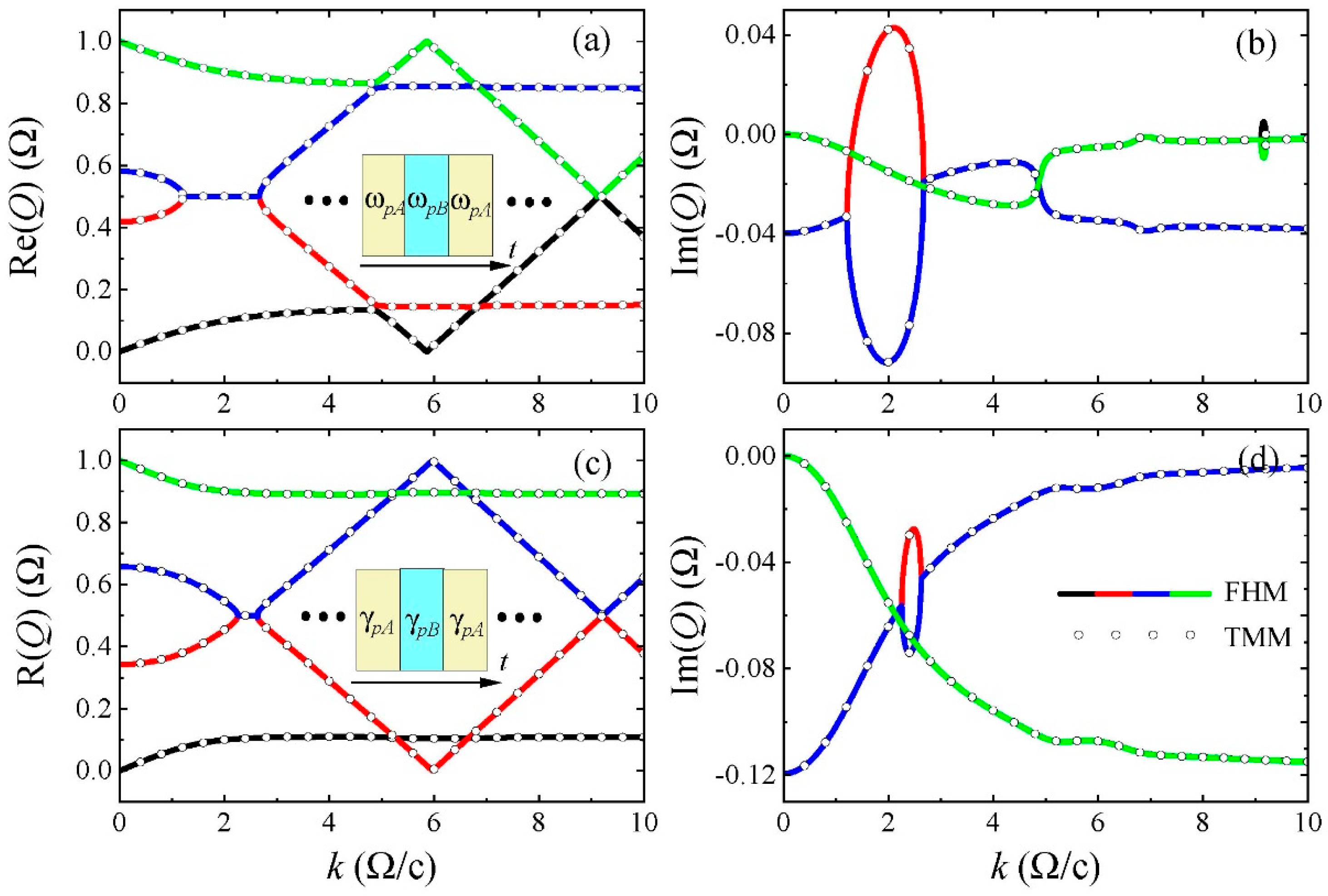
30] when the PTC exhibits step-like temporal boundaries. As an example, we consider that the PTC comprises two temporal sublayers (labeled as A and B) with equal time durations in each unit cell. In this scenario,
where
(
) are the plasma frequency and damping rate of layer A (B). In
Figure 1a,b, the real and imaginary parts of quasienergy bands correspond to the scenario where the plasma frequencies in the two sublayers are different, while the damping rate is nonzero and time-invariant. In contrast,
Figure 1c,d display the real and imaginary parts of the quasienergy bands when the damping rates in the two sublayers are different, while the plasma frequency remains static. The bands calculated by using the Floquet Hamiltonian (Equation (14) or Equation (20)) and the temporal transfer matrix method are shown in color lines and black circles, respectively. Evidently, the circles only fall on the lines, indicating the consistency between these two methods. In the calculations above and hereafter, the Floquet Hamiltonian method is truncated to a 36 × 36 matrix, with the block
(
) positioned at its center. This truncation ensures quasienergy band accuracy in the first Floquet zone.
Unlike the temporal transfer matrix method, which can only handle systems with step-like temporal boundaries, the proposed Floquet Hamiltonian method can also accommodate systems that evolve gradually over time. And in fact, the Floquet Hamiltonian method is valid for any time-periodic functions of
and even
. For example, we consider that
and
vary sinusoidally in time as
, where
represents the modulation phase difference between the damping rate and plasma frequency. Since
, the dispersive PTC exhibits a net zero damping rate in a time average. The plasma frequency and damping rate are modulated synchronously and asynchronously when
, and
, respectively. According to Equations (6) and (16),
are null except
and
Therefore, the Floquet Hamiltonian is block tridiagonal and the couplings are primarily between harmonics that differ by 1 in their orders. According to Equation (20), the coupling blocks depend on , causing the quasienergy bands to vary with .
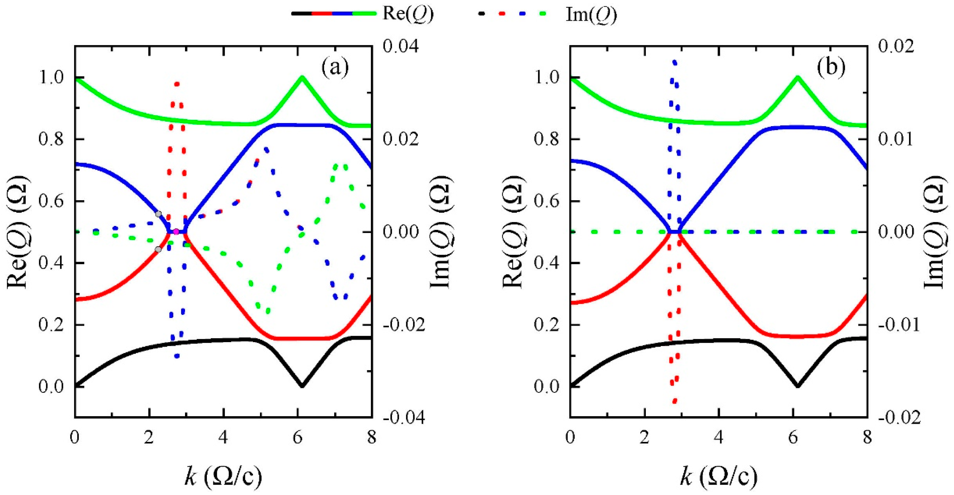
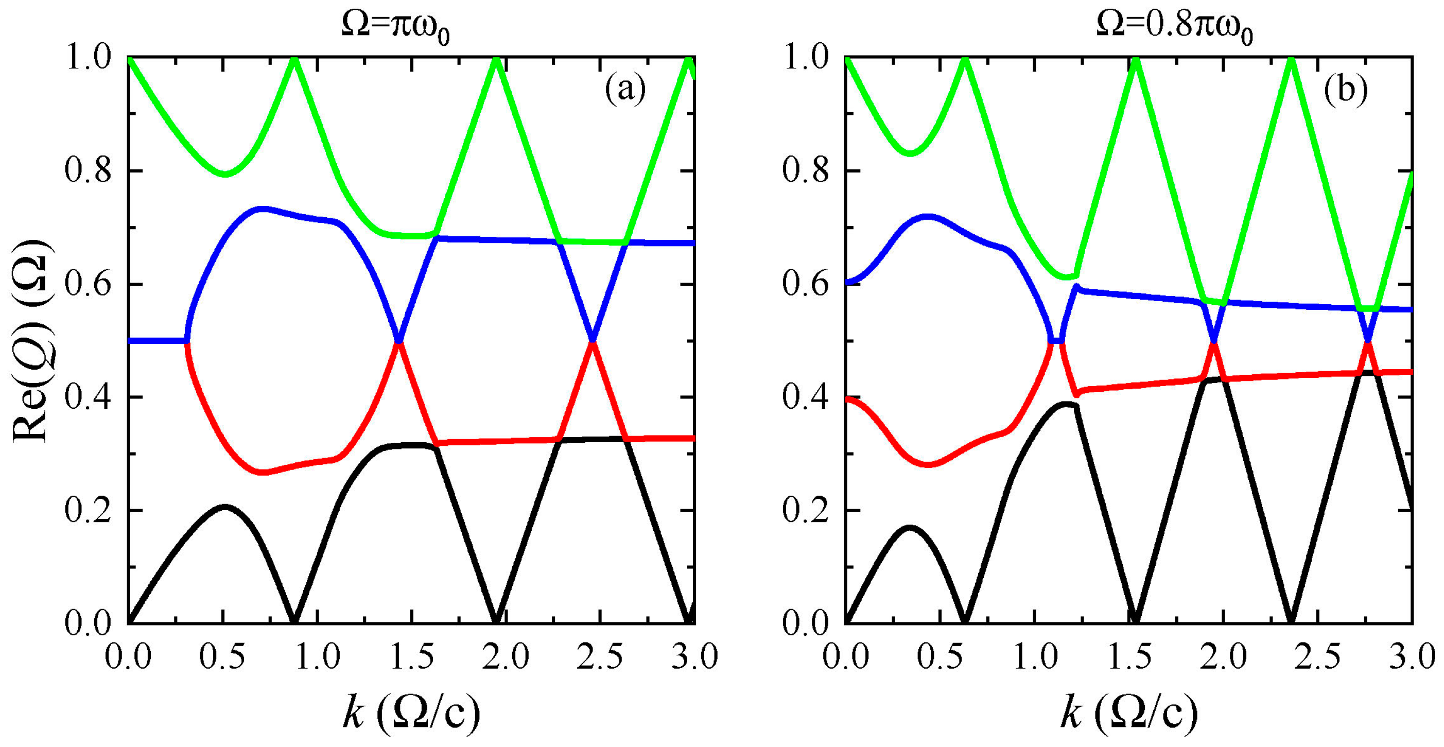
In
Figure 2a,b, we plot the quasienergy bands in the first Floquet zone for
and
, respectively. The parameters are set as
and
. The solid and dotted lines represent the real and imaginary parts, respectively, with the same color indicating the same band. When
, the quasienergy bands are entirely complex except at some isolated k points. In contrast, when
, the quasienergy bands are entirely real except those inside the k-gap, as shown in
Figure 2b. Moreover, the k-gap width is narrower than
. From Equations (A1)–(A3) in the
Appendix A, we observe that the
elements are all real, while the
elements are imaginary. Therefore, when
, the
elements become complex, causing the Floquet Hamiltonian
to be complex as well. As a result, the eigenvalues of
, also known as the quasienegies, are generally complex. However, when
, the blocks
is real, as well as
. Hence, the quasienergies are either real or in complex conjugate pairs.
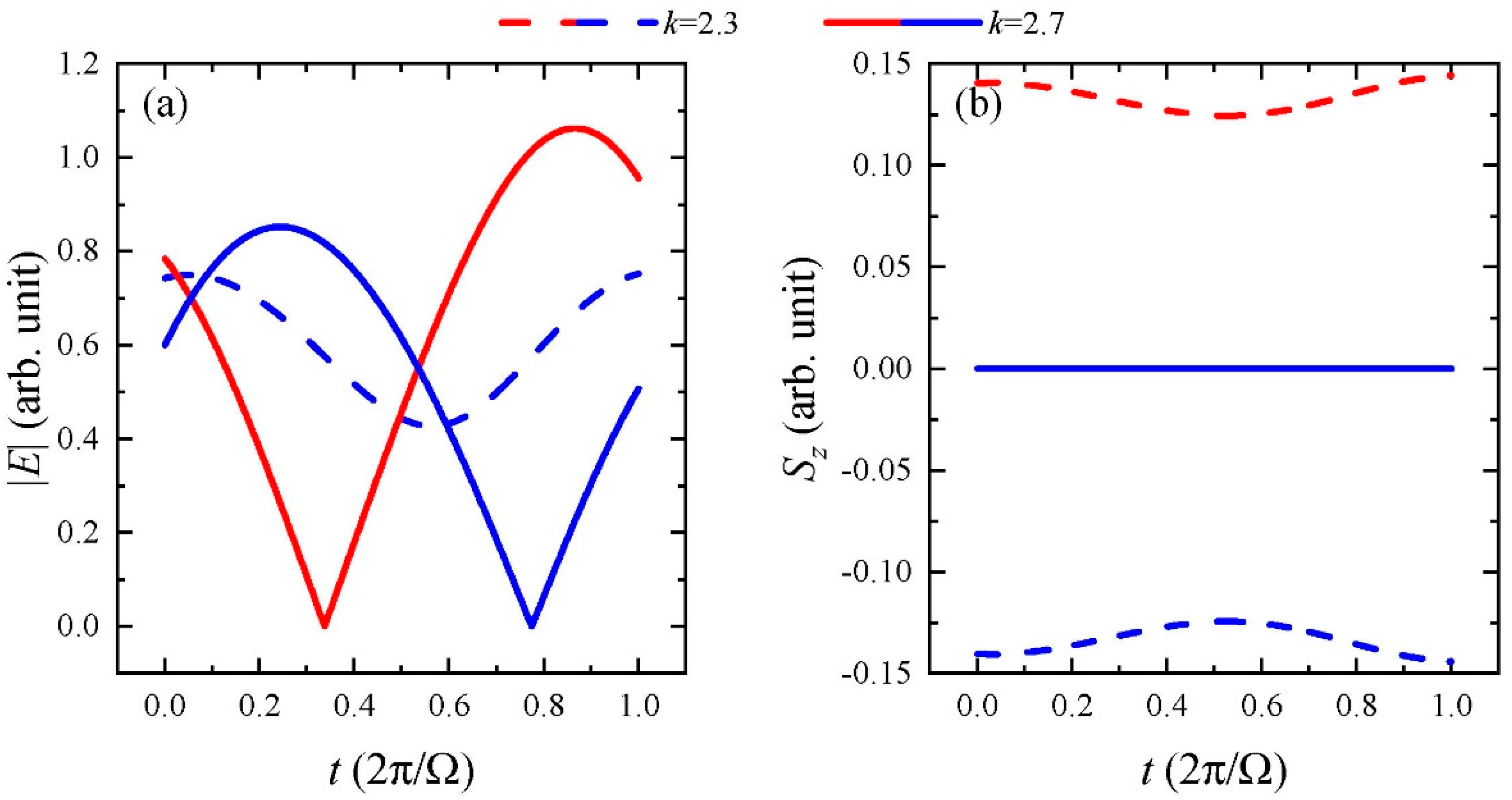
The electromagnetic fields for Floquet eigenstates are calculated according to Equation (9). We focused on the Floquet states of the second and third bands (red and blue lines in
Figure 2a) at
and
, which are outside and within the first k-gap, respectively. The electric field amplitudes are plotted in
Figure 3a. As shown with the dashed lines in
Figure 3a, outside the k-gap, the electric field amplitudes increase slightly after a modulation time period, since the quasienergies possess a small positive imaginary part; see
Figure 2a. In contrast, inside the k-gap, the electric amplitude for the second band is evidently enlarged, while that for the third band is reduced after a modulation time period, as shown with the solid lines in
Figure 3a. This is inside the k-gap, because
is positive for the second band while it is negative for the third band, as shown in
Figure 2a, resulting in field-amplifying and decaying behaviors.
We also calculate the energy fluxes of the Floquet states, expressed as
, and plot them as functions of time in
Figure 3b. For
, the energy flux for the second band (red dashed line) is positive while that for the third band (blue dashed line) is negative at all times, indicating that the corresponding Floquet states are propagating forward and backward, respectively. This aligns with the sign of the group velocity,
, which is positive for the second band and negative for the third band, as shown in
Figure 2a. On the other hand, the energy fluxes for the two bands inside the k-gap (
) are both vanishing at all times, as shown with the solid lines in
Figure 3b, indicating that the Floquet states are not propagative. This is also expected, since the real parts of quasienergy bands are flat inside the k-gap, as shown in
Figure 2a, rendering zero group velocities.
Additionally, the Floquet Hamiltonian method can also be used for directly calculating the left eigenstates
, according to the following [
32]
which is unachievable for the temporal transfer matrix method. For the temporal transfer matrix method, an alternative method is to construct an adjoint system first, and then obtain the right eigenstates of the adjoint system as the left eigenstate of the original system [
33]. The left eigenstates are necessary for calculating the phase rigidities [
6] and topological invariants of bands [
33], and the Green’s functions of the system [
1,
34].
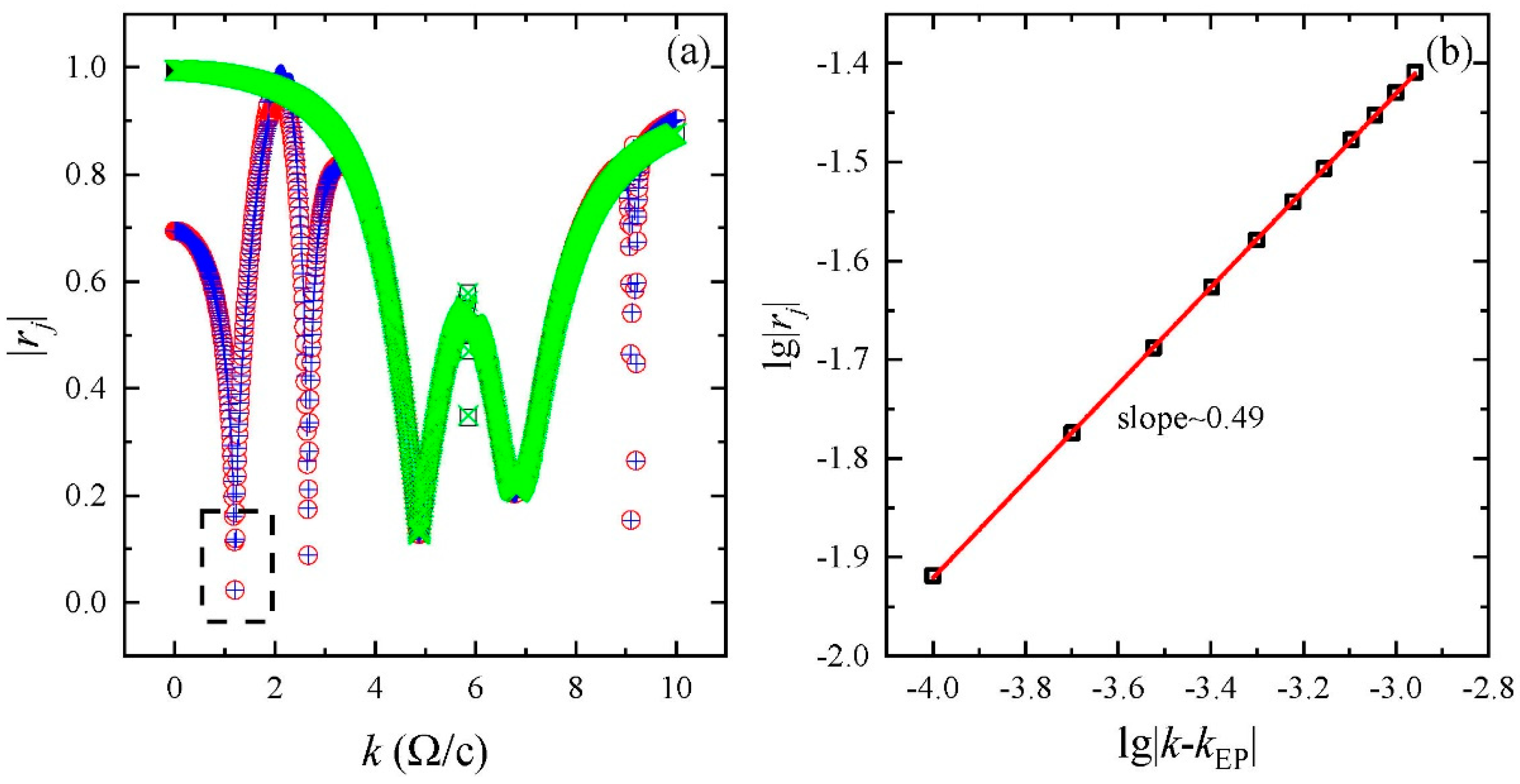
Figure 4a depicts the phase rigidities of the four bands in
Figure 1a. The phase rigidity of the
jth band is calculated as follows [
32]
The phase rigidities vanish at the first k-gap edges, indicating that the two k-gap edges correspond to a pair of exceptional points. Moreover, the order of the exceptional points can be justified according to the scaling exponent of the phase rigidities.
Figure 4b shows a log_log plot of the phase rigidities against the wavenumber deviation from the left k-gap edge. The plot exhibits excellent linearity, with a slope approximating 0.5, indicating that the exceptional point is of the second order.
4. Discussion
The emergence of EPs and k-gaps can be understood through the reduced Hamiltonian method [
5], which only accounts for the coupling between two coalesced bands when they are well separated from other bands in the quasienergy space. This condition applies to the bands within the first k-gaps in
Figure 1 and
Figure 2. According to Equation (17), the reduced Hamiltonian in this case is given as follows:
where
is the element of the coupling matrix
in the third row and fourth column, while
is the element of
in the fourth row and third column, and
are eigenfrequencies of
satisfying
. When the damping rate is zero in the static case (
), using Equation (A3), we obtain the following:
It is worth noting that the plasma frequency
and damping rate
are all purely real, which imposes the conditions
. It is evident that for either a nonzero
(modulated plasma frequency) or a nonzero
(modulated damping rate), the coupling between the two band is non-Hermitian as
. This non-Hermitian coupling leads to the emergence of EPs. Additionally, when the two bands cross, the relation
holds. Therefore, combining Equations (23), (24) and (A1), the quasienergies predicted by the reduced Hamiltonian are expressed as follows:
where
Since
is real,
is also real and generally negative, resulting in the quasienergies
forming a complex conjugate pair. The real parts of the k-gap are flat and positioned at the center of the first Floquet zone, consistent with the results shown in
Figure 1 and
Figure 2.
The Floquet Hamiltonian method is rigorous regardless of the modulation frequency amplitude, in contrast to the effective Hamiltonian method derived from the perturbation theory which is only applicable to high modulation frequencies [
35]. However, as
decreases, the bands of different harmonics move closer together, resulting in more complex interactions. In this scenario, the Floquet Hamiltonian matrix must be truncated to a larger size to preserve accuracy, as interactions from higher harmonic bands can no longer be ignored. Furthermore, the quasienergy bands undergo significant changes. As illustrated in
Figure 5a, when the modulation frequency decreases from
to
, the first k-gap in
Figure 2a shifts toward the small wavenumber region and merges with the k-gap at
, forming a wide k-gap. However, as the modulation frequency continues to decrease, this wide k-gap disappears, as shown in
Figure 5b, and a large quasienergy band gap opens at k = 0. These findings demonstrate that both k-gaps and quasienergy gaps can be effectively controlled by tuning the modulation frequency.
The Floquet Hamiltonian method can also handle scenarios involving multiple time modulation periods, such as when the plasma frequency and damping rate modulate at different frequencies. However, this requires that all these modulation periods be contained within a larger, overarching period, as this method is only applicable to time-periodic systems.
Although the proposed Floquet Hamiltonian method is effective for analyzing quasienergy bands and Floquet modes, its efficiency decreases when dealing with time-varying media that involve temporal or spatial boundaries. The TTMM is more efficient for a medium with finite temporal layers [
24]. However, in addition to the Floquet Hamiltonian analysis, a kick operator must be included to account for the scattering effects at the temporal boundaries [
35]. Moreover, both the Floquet Hamiltonian method and TTMM are ineffective when the medium encounters a spatial boundary. In such cases, the FDTD method is nearly irreplaceable.
