Transient Heat Transfer Modeling of SERF Co-Magnetometer Atomic Ensemble Based on the Thermoelectric Analogy Method

Abstract

Bias instability is one of the most critical factors in the performance of spin-exchange relaxation-free (SERF) co-magnetometers. Previous studies on SERF co-magnetometers have shown that changes in the atomic ensemble temperature can lead to variations in the alkali metal atom density, which in turn affect the optical rotation angle and light shift, ultimately influencing the system’s stability. Building on this understanding, this paper introduces the thermoelectric analogy method for the first time in the transient heat transfer analysis of SERF co-magnetometer atomic ensembles. Using this method, the primary factors affecting the atomic ensemble temperature in a SERF co-magnetometer were analyzed, and transient heat transfer models were established for the following processes: the interaction between the non-magnetic electric heating system and the atomic ensemble temperature, laser heating of the atomic ensemble by the optical system, and the effect of environmental temperature changes on the non-magnetic electric heating system. These models were experimentally validated through active temperature variation experiments. The experimental results show that the proposed transient heat transfer models accurately describe the related heat transfer processes of the atomic ensemble, with model fitting accuracy exceeding 98%. This lays a solid foundation for the high-precision closed-loop control of the atomic ensemble temperature in SERF co-magnetometers and provides valuable insights for the structural design and engineering applications of SERF co-magnetometers.

1. Introduction

With the deepening of theoretical research and technological advancements in the field of quantum control, atomic sensors have attracted extensive attention in related areas such as inertial navigation, physical research, magnetic field measurement, and imaging, with some atomic sensors already entering engineering applications [1,2,3]. Atomic inertial measurement instruments, which have developed rapidly in recent years, are considered the future direction of inertial navigation systems due to their outstanding advantages of a high performance and low cost [4,5,6]. In quantum sensors, the decoherence and relaxation of qubits are among the main sources of errors. The realization of the SERF state eliminates the atomic spin-exchange collision relaxation term, which plays a dominant role in the relaxation of alkali-metal atoms, thus significantly reducing the atomic relaxation rate, extending the coherence time of atoms, and improving the ultimate sensitivity in magnetic field measurements based on atomic spins. Compared with existing high-precision inertial measurement systems, SERF co-magnetometers show tremendous potential for ultra-high precision in the same volume and ultra-small volume for the same precision.

The alkali-metal vapor cell is the sensitive core of the SERF co-magnetometer. The temperature of the atomic ensemble inside the vapor cell determines key parameters such as the number density and average thermal motion speed of the alkali-metal atoms, making it one of the main factors influencing the stability and sensitivity of the SERF-based inertial measurement system. Firstly, atomic density undergoes significant changes with temperature, which has a crucial impact on the atomic relaxation terms [7]. Additionally, the center frequency and linewidth of the atomic absorption spectrum change with the temperature of the atomic ensemble, thereby altering the optical pumping rate and the optical rotation angle [8]. High-precision closed-loop temperature control of the atomic ensemble is an effective solution to this issue. Establishing a transient heat transfer model for the atomic ensemble is fundamental for achieving high-precision temperature stability control of the ensemble. In a SERF co-magnetometer with a $\mathrm{K}-\mathrm{Rb}-{}^{21}\mathrm{Ne}$ atomic source, the alkali-metal atomic vapor cell is typically heated to over 160 °C using a non-magnetic electric heater in order to achieve the SERF state, while the surrounding environment is usually 23–25 °C. This creates a coexistence of high and low temperatures from the alkali-metal atomic ensemble to the system surface, leading to a complex thermal field. Furthermore, the heating effects of the pump and detection lasers on the atomic ensemble’s temperature stability cannot be ignored. These factors present significant challenges for the establishment and analysis of a transient heat transfer model for the atomic ensemble.

In the field of inertial measurement, methods for modeling unsteady-state heat transfer primarily include finite difference methods, finite element methods, finite volume methods, and machine learning approaches. Weiwei Wang et al. used the finite element method to derive a simplified M-C-K dynamic model for MEMS gyroscopes, presenting the relationship between resonance frequency shift and temperature variation at a reference temperature of 20 °C [9]. Jun Ma et al. proposed a temperature modeling and compensation method based on a multi-layer perceptron. After compensation using this model, the gyroscope’s bias stability improved by 80% [10]. Mu Jiao Ouyang et al. developed temperature compensation models for gyroscope output signals using Long Short-Term Memory (LSTM) networks, Support Vector Machines (SVMs), and Deep Belief Networks (DBNs). The compensation reduced the rate random drift and bias instability of the gyroscope output signals by 84.35% and 95.57%, respectively [11]. However, these methods are computationally complex and difficult to express theoretically.

In contrast, analog theory plays an important role in transient heat transfer calculations, where heat is transferred in the form of waves. Thermoelectric analog computations are relatively simpler and are commonly used for solving unsteady-state heat transfer problems. Existing techniques and solutions from the electrical domain can be applied to address heat transfer issues. The use of thermoelectric analogy for transient heat transfer analysis has broad applications across various fields. Jiaojiao Duan et al., based on the thermoelectric analogy mechanism and the principles of circuit transient analysis, established a full-response model for wall heat transfer analysis [12]. The model was validated by comparing it with the experimental results. G. Fress et al. proposed a novel thermoelectric element modeling method based on thermoelectric analogy, which is applicable for steady-state descriptions as well as for transient and unconventional geometries [13]. Kehui Zhou et al. applied thermoelectric analogy theory and lumped parameter models to establish a hotspot temperature model for the outer wall of transformers [14]. Through analyzing experimental data, they developed a mathematical model that describes the impact of environmental temperature and wind speed on transformer temperature, obtaining corrected temperature values for the transformer under different environmental conditions and wind speeds.

This paper, based on the practical conditions of a SERF co-magnetometer, conducts transient heat transfer modeling and experimental validation using the thermoelectric analogy method to investigate the variables affecting the temperature of the atomic ensemble in a SERF co-magnetometer. The goal is to lay the foundation for high-precision closed-loop temperature control of the atomic ensemble in a SERF co-magnetometer. Experimental results demonstrate that the full-response model of the atomic ensemble temperature, established using the thermoelectric analogy method, aligns well with the experimental data, validating the effectiveness of the modeling approach.

The remainder of this paper is organized as follows: In Section 2, we begin with the structure of the SERF co-magnetometer and develop a transient heat transfer full-response model for the atomic ensemble temperature using the thermoelectric analogy method. Section 3 describes the experimental setup and methods. Section 4 presents the experimental validation results. Finally, our conclusions are provided in Section 5.

2. Model Overview

2.1. Error Analysis of the Atomic Ensemble Temperature in a SERF Co-Magnetometer

In a SERF co-magnetometer with an atomic source of $\mathrm{K}-\mathrm{Rb}-{}^{21}\mathrm{Ne}$, the atomic density of the alkali-metal atoms is highly dependent on the temperature of the atomic ensemble. Changes in the alkali-metal atomic density affect the steady-state output of the SERF co-magnetometer through the optical rotation angle $\theta$. The relationship between the steady-state output S and the alkali-metal atomic density $N_{Rb}$ can be expressed by Equation (1) [15].

$$S=-2\eta G{I}_0{\displaystyle \frac{1}{2}}lc{r}_e{f}_{D1}^{Rb}{N}_{Rb}{P}_x^{\mathrm{e}}{e}^{-N_{Rb}\sigma (v_0)l}{\displaystyle \frac{v_{pr}-v_{D1}^{Rb}}{{\left(v_{pr}-v_{D1}^{Rb}\right)}^2+{\left({\Gamma }_{D1}^{Rb}/2\right)}^2}}$$

(1)

where l is the length of the laser path through the atomic ensemble, $r_e$ is the classical electron radius, c is the speed of light, $f_{D1}^{Rb}$ is the oscillator strength of the $\mathrm{Rb}$ atomic D1 line, $N_{Rb}$ is the number density of $\mathrm{Rb}$ atoms, $P_x^{\mathrm{e}}$ is the steady-state polarization, $v_{pr}$ is the center frequency of the detection laser, $v_{D1}^{Rb}$ is the center frequency of the $\mathrm{Rb}$ atomic D1 line, ${\Gamma }_{D1}^{Rb}$ is the pressure broadening of the $\mathrm{Rb}$ atomic D1 line, $\eta$ is the conversion efficiency of the optical signal to an electrical signal, G is the amplification factor, $I_0$ is the light intensity before the detection laser enters the atomic ensemble, and $\sigma (v_0)$ is the absorption cross-section of the light. Changes in the alkali-metal atomic density also affect the light shift, which can lead to crosstalk between the two sensitive axes.

In addition, the light shift influences the linewidth and sensitivity of the co-magnetometer. The relationship between the light shift and the alkali-metal atomic density is shown in Equation (2) [16].

$$L_z=L_z^{Rb}+{\displaystyle \frac{N_K}{N_{Rb}}}{L}_z^K$$

(2)

where $L_z^{Rb}$ is the light shift for species $\mathrm{Rb}$ and $L_z^K$ is the atomic light shift for species $\mathrm{K}$. In summary, fluctuations in the atomic ensemble temperature can introduce various errors in the SERF co-magnetometer, and it is essential to analyze the main factors that cause these temperature fluctuations.

2.2. Thermoelectric Analogy Analysis and Modeling

The non-magnetic electric heating system, active and passive magnetic shielding systems, and the main structure are generally composed of multiple layers of materials, each with specific thermal resistance and thermal capacity, similar to the electrical resistance and capacitance of conductive components. Therefore, the heat transfer models for each part can be analogous to the circuit models of conductive components and transformed into RC network nodes. The primary thermal sources affecting the atomic ensemble in the SERF co-magnetometer can be treated as voltage sources. In this study, a 4R2C double-layer T-shaped RC network, a 2R1C single-layer T-shaped RC network, and a 14R7C seven-layer T-shaped RC network are used to analyze the main influencing factors.

2.2.1. Transient Heat Transfer Analysis of the Non-Magnetic Electric Heating System and Atomic Ensemble

The non-magnetic electric heating system consists, from the outside in, of a non-magnetic heating film driven by high-frequency alternating current, a high thermal conductivity ceramic oven, and a glass vapor cell containing the atomic ensemble, which is placed inside the ceramic oven. The non-magnetic heating film is tightly wrapped around the surface of the high thermal conductivity ceramic oven. The heat transfer process between the non-magnetic electric heating and the atomic ensemble can be analyzed using a thermal circuit model represented by a 4R2C double-layer T-shaped RC network. The double-layer T-shaped RC network represents the high thermal conductivity ceramic oven and the glass vapor cell, with the non-magnetic heating film temperature acting as the voltage source, as shown in Figure 1.

Based on Kirchhoff’s Current Law (KCL), the heat transfer between the non-magnetic electric heating and the atomic ensemble is determined by Equations (3)–(5).

$$C_1{\displaystyle \frac{d{T}_1}{dt}}={\displaystyle \frac{T_{heat}-T_1}{R_1/2}}-{\displaystyle \frac{T_1-T_2}{R_1/2}}$$

(3)

$${\displaystyle \frac{T_1-T_2}{R_1/2}}={\displaystyle \frac{T_2-T_3}{R_2/2}}$$

(4)

$$C_2{\displaystyle \frac{d{T}_3}{dt}}={\displaystyle \frac{T_2-T_3}{R_2/2}}-{\displaystyle \frac{T_3-T_{cell}}{R_2/2}}$$

(5)

In the equations, $C_1$ represents the heat capacity of the oven wall; $R_1$ is the thermal resistance of the oven; $C_2$ is the heat capacity of the oven; $R_2$ is the thermal resistance of the vapor cell; and $T_{\mathrm{heat}}$, $T_1$, $T_2$, $T_3$, and $T_{\mathrm{cell}}$ represent the temperatures of the heating film, node 1, the inner wall temperature of the oven, node 3, and the atomic ensemble temperature, respectively. The temperatures at each node can be obtained by solving Equations (6)–(8).

$$T_1=({T_1}^0-{\displaystyle \frac{T_{heat}+T_2}{2}})e^{-{\displaystyle \frac{4}{C_1{R}_1}}t}+{\displaystyle \frac{T_{heat}+T_2}{2}}$$

(6)

$$T_2={\displaystyle \frac{R_2{T}_1+R_1{T}_3}{R_1+R_2}}$$

(7)

$$T_3=({T_3}^0-{\displaystyle \frac{T_2+T_{cell}}{2}})e^{-{\displaystyle \frac{4}{C_2{R}_2}}t}+{\displaystyle \frac{T_2+T_{cell}}{2}}$$

(8)

In the equations, ${T_1}^0$ and ${T_3}^0$ represent the initial temperatures of node 1 and node 3, respectively. By solving Equations (6)–(8) simultaneously, the heat transfer model for the non-magnetic electric heating system and the atomic ensemble temperature can be obtained:

$$T_{cell}={\displaystyle \frac{(e^{-k_{1}t}{R}_2-R_2)T_{heat}+[(e^{-k_{1}t}+1)R_2+(e^{-k_{2}t}+1)R_1]T_2-2e^{-k_{1}t}{R}_2{T_1}^0-2e^{-k_{2}t}{R}_1{T_3}^0}{R_1(1-e^{-k_{2}t})}}$$

(9)

where $k_1={\displaystyle \frac{4}{C_1{R}_1}}$; $k_2={\displaystyle \frac{4}{C_2{R}_2}}$

2.2.2. Analysis of Laser Heating in the Optical System and Heat Transfer to the Atomic Ensemble

As the laser beam passes through the glass vapor cell and the atomic ensemble, it simultaneously heats both the walls of the glass vapor cell and the atomic ensemble inside it. Therefore, a comprehensive analysis of both the glass vapor cell wall and the atomic ensemble is required. The heat transfer from the laser heating to the atomic ensemble is modeled using a 2R1C single-layer T-shaped RC network for analysis, as shown in Figure 2 below.

Based on KCL, the heat transfer from the laser heating to the atomic ensemble is determined by Equation (10).

$$C_3{\displaystyle \frac{d{T}_{cell}}{dt}}={\displaystyle \frac{T_{p1}-T_{cell}}{\frac{R_3}{2}}}-{\displaystyle \frac{T_{cell}-T_{p2}}{\frac{R_3}{2}}}$$

(10)

where $C_3$ represents the overall heat capacity of the glass vapor cell and atomic ensemble; $R_3$ is the overall thermal resistance between the glass vapor cell and the atomic ensemble; and $T_{p1}$ and $T_{p2}$ represent the temperatures at the point where the laser enters the vapor cell and where it exits, respectively. The heat transfer model for the atomic ensemble temperature due to laser heating can be obtained by solving Equation (11).

$$T_{cell}=({T_{cell}}^0-{\displaystyle \frac{T_{p1}+T_{p2}}{2}})e^{-k_{3}t}+{\displaystyle \frac{T_{p1}+T_{p2}}{2}}$$

(11)

where $k_3={\displaystyle \frac{4}{C_3{R}_3}}$; ${T_{cell}}^0$ is the initial temperature of the atomic ensemble.

2.2.3. Analysis of Heat Transfer Between Environmental Temperature and the Non-Magnetic Electric Heating System

The environmental temperature affects the temperature of the SERF co-magnetometer shell, main structure, three-layer magnetic shielding cylinder, active magnetic compensation coils, and the non-magnetic electric heating support structure from the outside in, thereby influencing the temperature of the non-magnetic electric heating system. In this paper, the heat transfer between the environmental temperature and the non-magnetic electric heating system is modeled using a 14R7C seven-layer T-shaped RC network, as shown in the Figure 3 below. Based on Kirchhoff’s law, and following the analysis methods described earlier in this paper, the transient heat transfer models for each node are directly presented in their simplified form and represented using state-space matrices.

$$\begin{array}{c}\left[\begin{array}{cccccc}{\displaystyle \frac{k_6{R}_4}{k_5{R}_4+k_4{R}_5}}& 0& 0& 0& 0& 0\\ {\displaystyle \frac{k_6{R}_6}{k_7{R}_5+k_5{R}_6}}& {\displaystyle \frac{k_8{R}_5}{k_7{R}_5+k_5{R}_6}}& 0& 0& 0& 0\\ 0& {\displaystyle \frac{k_8{R}_7}{k_7{R}_7+k_9{R}_6}}& {\displaystyle \frac{k_{10}{R}_6}{k_7{R}_7+k_9{R}_6}}& 0& 0& 0\\ 0& 0& {\displaystyle \frac{k_{10}{R}_8}{k_9{R}_8+k_{11}{R}_7}}& {\displaystyle \frac{k_{12}{R}_7}{k_9{R}_8+k_{11}{R}_7}}& 0& 0\\ 0& 0& 0& {\displaystyle \frac{k_{12}{R}_9}{k_{11}{R}_9+k_{13}{R}_8}}& {\displaystyle \frac{k_{14}{R}_8}{k_{11}{R}_9+k_{13}{R}_8}}& 0\\ 0& 0& 0& 0& {\displaystyle \frac{k_{14}{R}_{10}}{k_{13}{R}_{10}+k_{15}{R}_9}}& {\displaystyle \frac{k_{16}{R}_9}{k_{13}{R}_{10}+k_{15}{R}_9}}\end{array}\right]\left[\begin{array}{c}{T}_5\\ T_7\\ T_9\\ T_{11}\\ T_{13}\\ T_{15}\end{array}\right]\hfill \\ =\left[\begin{array}{c}{\displaystyle \frac{2R_5{e}^{-\frac{4}{C_4{R}_4}t}{T_4}^0+2R_4{e}^{-\frac{4}{C_5{R}_5}t}{T_6}^0+R_5(1-e^{-\frac{4}{C_4{R}_4}t})T_{evn}}{k_5{R}_4+k_4{R}_5}}\\ {\displaystyle \frac{2R_6{e}^{-\frac{4}{C_5{R}_5}t}{T_6}^0+2R_5{e}^{-\frac{4}{C_6{R}_6}t}{T_8}^0}{k_7{R}_5+k_5{R}_6}}\\ {\displaystyle \frac{2R_7{e}^{-\frac{4}{C_6{R}_6}t}{T_8}^0+2R_6{e}^{-\frac{4}{C_7{R}_7}t}{T_{10}}^0}{k_7{R}_7+k_9{R}_6}}\\ {\displaystyle \frac{2R_8{e}^{-\frac{4}{C_7{R}_7}t}{T_{10}}^0+2R_7{e}^{-\frac{4}{C_8{R}_8}t}{T_{12}}^0}{k_9{R}_8+k_{11}{R}_7}}\\ {\displaystyle \frac{2R_9{e}^{-\frac{4}{C_8{R}_8}t}{T_{12}}^0+2R_8{e}^{-\frac{4}{C_9{R}_9}t}{T_{14}}^0}{k_{11}{R}_9+k_{13}{R}_8}}\\ {\displaystyle \frac{2R_{10}{e}^{-\frac{4}{C_9{R}_9}t}{T_{14}}^0+2R_9{e}^{-\frac{4}{C_{10}{R}_{10}}t}{T_{16}}^0}{k_{13}{R}_{10}+k_{15}{R}_9}}\end{array}\right]\hfill \end{array}$$

(12)

where $k_4=1+e^{-{\displaystyle \frac{4}{C_4{R}_4}}t};$ $k_5=1+e^{-{\displaystyle \frac{4}{C_5{R}_5}}t};$ $k_6=1-e^{-{\displaystyle \frac{4}{C_5{R}_5}}t};$ $k_7=1+e^{-{\displaystyle \frac{4}{C_6{R}_6}}t}; k_8=1-e^{-{\displaystyle \frac{4}{C_6{R}_6}}t};$ $k_9=1+e^{-{\displaystyle \frac{4}{C_7{R}_7}}t};$ $k_{10}=1-e^{-{\displaystyle \frac{4}{C_7{R}_7}}t};$ $k_{11}=1+e^{-{\displaystyle \frac{4}{C_8{R}_8}}t};$ $k_{12}=1-e^{-{\displaystyle \frac{4}{C_8{R}_8}}t};$ $k_{13}=1+e^{-{\displaystyle \frac{4}{C_9{R}_9}}t};$ $k_{14}=1-e^{-{\displaystyle \frac{4}{C_9{R}_9}}t};$ $k_{15}=1+e^{-{\displaystyle \frac{4}{C_{10}{R}_{10}}}t};$ $k_{16}=1-e^{-{\displaystyle \frac{4}{C_{10}{R}_{10}}}t};$ $T_4$ to $T_{16}$ represent the temperatures of node 4, the main structure, node 6, the first layer of permalloy magnetic shielding, node 8, the second layer of permalloy, node 10, the ferrite magnetic shielding cylinder, node 12, the active magnetic compensation coils, node 14, the oven support, and node 16, respectively. $R_4$ to $R_{10}$ represent the thermal resistances of the shell, main structure, first layer of permalloy magnetic shielding cylinder, second layer of permalloy magnetic shielding cylinder, ferrite magnetic shielding cylinder, active magnetic compensation coils, and oven support, respectively. $C_4$ to $C_{10}$ represent the thermal capacities of the shell, main structure, first layer of permalloy magnetic shielding cylinder, second layer of permalloy magnetic shielding cylinder, ferrite magnetic shielding cylinder, active magnetic compensation coils, and oven support, respectively. ${T_n}^0$ represents the initial temperatures of the nodes.

2.3. Determination of RC Heat Transfer Network Parameters

Thermal resistance represents the temperature difference generated under a unit heat flow rate, similar to how electrical resistance represents the voltage difference produced under a unit current. Thermal capacitance represents the ability of a body to store thermal energy, analogous to how electrical capacitance represents the ability to store charge. The values of thermal resistance and thermal capacitance can be calculated using Equations (13) and (14).

$$R={\displaystyle \frac{L}{kA}}$$

(13)

$$C=mc$$

(14)

where L represents the length of the heat transfer path, k is the material’s thermal conductivity, A is the surface area through which heat flows, m is the material’s mass, and c is the specific heat capacity of the material. The reference values for the RC parameters of the various components of the SERF co-magnetometer are shown in

Table 1. Reference RC values for the components of the SERF co-magnetometer.

Name	Material	Thermal Resistance R (K/W)	Thermal Capacity C (J/K)
Oven	Boron Nitride Ceramic	0.114	29.37
Glass Vapor Cell	Borosilicate Glass	0.057	0.128
Atomic Ensemble	Gas	437	0.00062
Shell	Titanium Alloy	0.33	16124
Main Structure	Titanium Alloy	0.52	6342
First Layer Magnetic Shielding Cylinder	Permalloy	1.48	2687
Second Layer Magnetic Shielding Cylinder	Permalloy	1.79	2164
Third Layer Magnetic Shielding Cylinder	Manganese Zinc Ferrite	6.12	632
Magnetic Compensation Coil	Polyether Ether Ketone	14.6	87
Oven Support	Polyether Ether Ketone	9.06	140

.

3. Experimental Setup

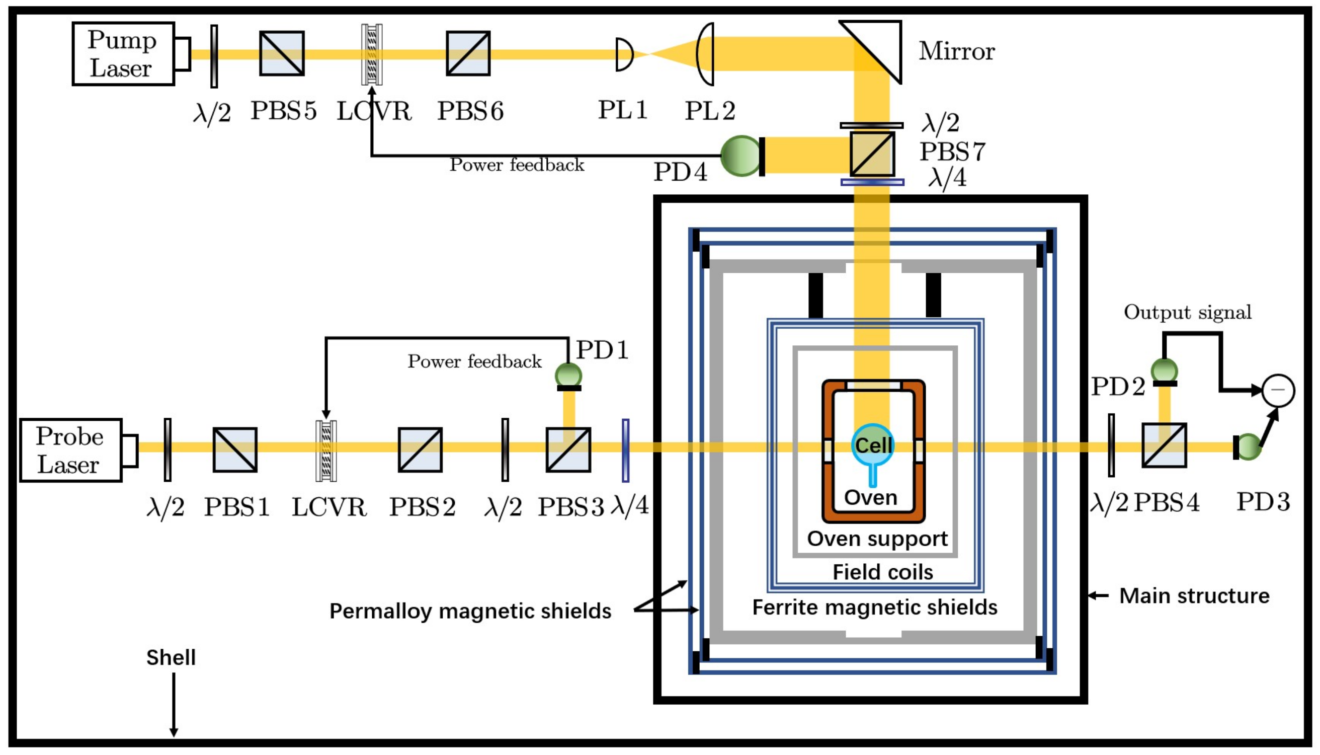
The SERF co-magnetometer experimental setup used in this work is shown in Figure 4. The magnetometer device used in the experiment includes a glass vapor cell containing potassium ($\mathrm{K}$), rubidium ($\mathrm{Rb}$), neon-21 (${}^{21}\mathrm{Ne}$), and nitrogen (${\mathrm{N}}_2$). This vapor cell is positioned at the core of the magnetometer, with an external heating oven made of boron nitride material. A platinum resistance sensor is installed on the oven to continuously monitor the temperature of the vapor cell, serving as a feedback element for the temperature control system. The heating of the vapor cell is achieved by a non-magnetic heating film wrapped around the outside of the oven, driven by a high-frequency alternating current. This heating film is controlled by a closed-loop feedback system, which precisely adjusts the vapor cell temperature by regulating the current through the heating film. A PID control system is used to maintain temperature fluctuations within 0.01 K. The oven is positioned at the center of three mutually perpendicular magnetic coils, with an external magnetic shielding system consisting of two layers of permalloy and one layer of ferrite. This passive magnetic shielding system works in conjunction with the active magnetic compensation system of the three coils to create a low magnetic field environment. In the experiment, potassium atoms are excited by a circularly polarized pump beam, which is polarized along the z-axis and emitted by a pump diode laser. The pump beam is Gaussian and is expanded using a beam-expanding lens system to select an area with a uniform light intensity, covering most of the vapor cell. The wavelength of the pump light is stabilized at the potassium D1 transition (approximately 770.1084 nm) using a saturation absorption system. Subsequently, rubidium atoms are polarized through spin-exchange interactions with potassium atoms, further polarizing neon-21 atoms through spin-exchange with rubidium atoms. The polarization of the electron spin in the x-direction is detected using the optical rotation effect of a non-resonant linearly polarized probe light beam emitted by the probe laser. The wavelength of the probe light is approximately 795.3495 nm, and optical differential detection technology is employed to accurately measure the polarization angle. Additionally, an optical power stabilization system (OPSS) is used to control the light power of both the pump and probe beams, ensuring the stability of the light intensity throughout the experiment. With this setup and control system, the experiment achieves high-precision detection of electron spin polarization in a low magnetic field environment, thereby supporting the high-sensitivity measurements of the magnetometer.

To verify the effectiveness of the method, we performed experimental validation of the transient heat transfer models for the non-magnetic electric heating system and atomic ensemble temperature, optical system laser heating and atomic ensemble temperature, and environmental temperature and non-magnetic electric heating system.

Step 1: The SERF co-magnetometer was placed in a temperature-controlled chamber to maintain environmental stability. The heating film was operated at full power. Three platinum resistance thermometers were placed on the surface of the heating film, the inner wall of the oven, and inside the glass vapor cell to monitor the temperature of the atomic ensemble. Temperature variations at the three points were monitored synchronously using a multi-channel temperature monitoring device. The measured temperature data were then fitted using Equation (10) and compared with the experimental results.

Step 2: The SERF co-magnetometer was similarly placed in the temperature-controlled chamber, and a Gaussian beam with a light power density of 5 mW/cm² was incident on the alkali metal vapor cell. Three platinum resistance thermometers were used to simultaneously monitor the temperature changes on the surface of the glass vapor cell, inside the glass vapor cell, and on the surface of the exiting glass vapor cell. The measured temperature data were fitted using Equation (12) and compared with the experimental results.

Step 3: The temperature of the heating film was stabilized at around 185 °C, and a 5 °C temperature variation was applied using the temperature-controlled chamber. Seven platinum resistance thermometers were used to simultaneously monitor the temperature changes in the SERF co-magnetometer’s casing, main structure, first layer of permalloy magnetic shielding tube, second layer of permalloy magnetic shielding tube, manganese-zinc ferrite magnetic shielding tube, active magnetic compensation coils, oven support, and heating film. The measured temperature data were fitted using Equation (13) and compared with the experimental results.

4. Results and Discussion

First, this paper validates the accuracy of the transient heat transfer model for the non-magnetic electric heating system and atomic ensemble, using the method outlined in Step 1. When the non-magnetic electric heating system operates at full power, the temperature variations in the heating film, oven inner wall, and atomic ensemble are shown in Figure 5.

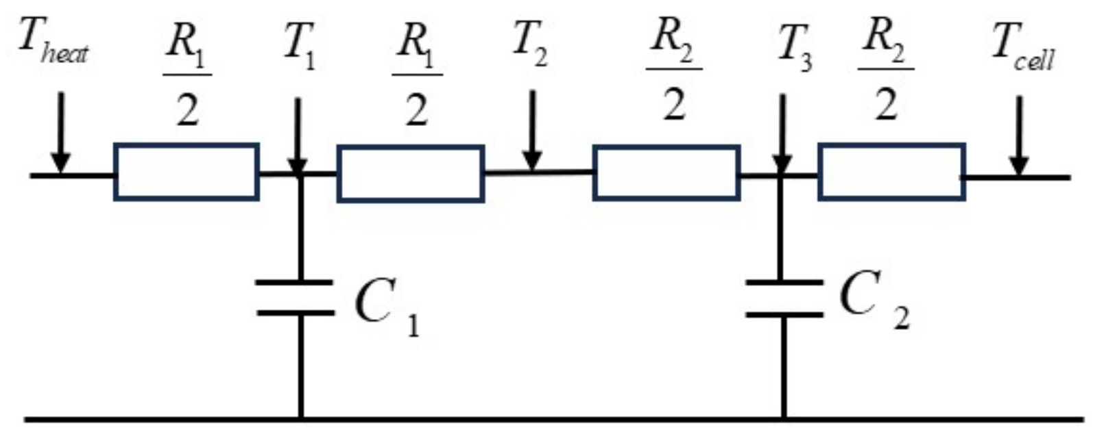
The red, blue, and pink curves in the figure represent the temperature changes of the heating film, oven wall, and atomic ensemble, respectively, under full-power heating of the non-magnetic electric heating system. The measured data were fitted using Equation (9), as shown in Figure 6. The root mean square error (RMSE) between the model fit curve and the measured curve was 0.44, which is only one-thousandth of the test range, indicating that the model closely matches the measured data. The 4R2C heat transfer network effectively describes the transient heat transfer process between the heating film and the atomic ensemble temperature.

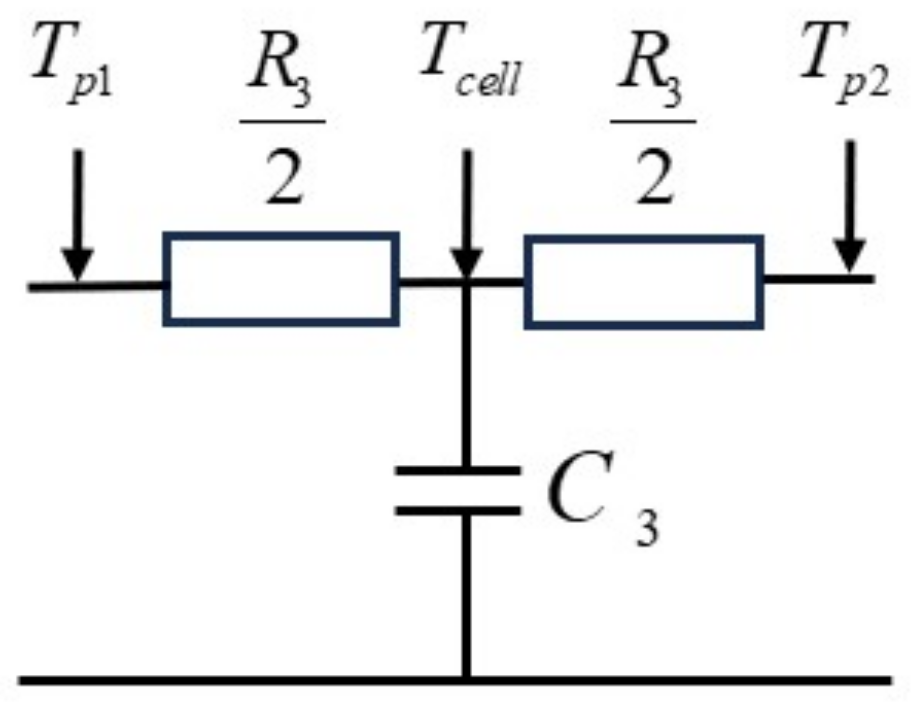
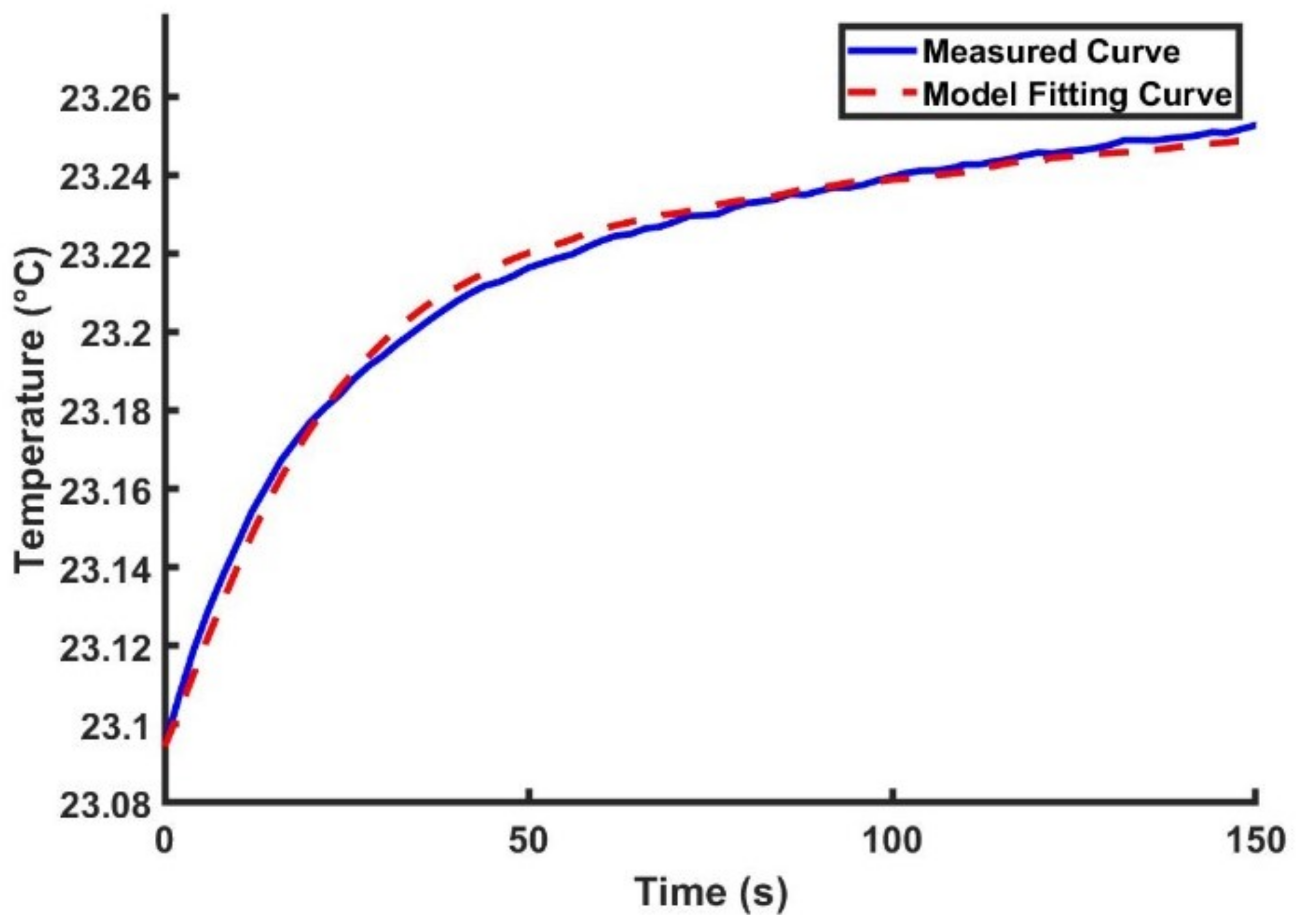
Next, we validate the accuracy of the transient heat transfer model for laser heating and the atomic ensemble using the method described in Step 2. When a Gaussian beam is incident on the alkali metal vapor cell, the temperature changes at the laser incidence surface, atomic ensemble, and laser exit surface are shown in Figure 7. The red, blue, and pink curves represent the temperature variations at the laser incidence surface, atomic ensemble, and laser exit surface, respectively. The measured data were fitted using Equation (11), as shown in Figure 8. The red dashed line represents the model fit curve. The RMSE between the model fit curve and the measured data is 0.000015, indicating a good agreement between the model and the measured data. The 2R1C heat transfer network effectively describes the transient heat transfer process between laser heating and atomic ensemble temperature.

Finally, we validate the accuracy of the transient heat transfer model for the non-magnetic electric heating system in conjunction with the environmental temperature, using the method outlined in Step 3. A 5 °C temperature variation was applied to the SERF co-magnetometer using a temperature-controlled chamber. The temperature variations of the environment temperature $T_{\mathrm{env}}$, main structure temperature $T_5$, first layer permalloy magnetic shield temperature $T_7$, second layer permalloy magnetic shield temperature $T_9$, ferrite magnetic shield temperature $T_{11}$, active magnetic compensation coil temperature $T_{13}$, oven support temperature $T_{15}$, and heating film temperature $T_{heat}$ are shown in Figure 9. The temperature variation data for each component with respect to the environmental temperature were fitted using Equation (12), and the results are shown in Figure 10.

The experimental results show that the root mean square errors (RMSE) between the model fitting results and the measured data for $T_5$, $T_7$, $T_9$, $T_{11}$, $T_{13}$ and $T_{15}$ are 0.000029, 0.000029, 0.000038, 0.00003, 0.000076, and 0.000038, respectively. This indicates a good agreement between the model and the measured results. The 14R7C thermal model can effectively describe the transient heat transfer process of the heating film temperature in response to changes in the environmental temperature.

5. Conclusions

This paper is the first to introduce the thermoelectric analogy method into the transient heat transfer analysis of the SERF co-magnetometer atomic ensemble. Using this method, we analyzed the primary factors affecting the temperature of the SERF co-magnetometer atomic ensemble, establishing transient heat transfer models for the non-magnetic electric heating system and atomic ensemble temperature, laser heating and atomic ensemble temperature, and environmental temperature with the non-magnetic electric heating system. These models were experimentally validated through active temperature variation experiments. The experimental results demonstrate that the proposed models accurately describe the relevant transient heat transfer processes, providing a solid foundation for the subsequent high-precision closed-loop control of the SERF co-magnetometer atomic ensemble temperature. Furthermore, these findings offer valuable insights for enhancing the long-term stability of the SERF co-magnetometer.

In future work, we will address the limitations imposed by the experimental setup structure and certain approximations in the model, the difficulties in obtaining actual RC parameters, and potential discrepancies between measured values and theoretical calculations. In addition, we plan to conduct temperature modeling for different light spot geometries to further enhance the generality and accuracy of the method. We will further refine the accuracy of the thermoelectric analogy modeling through fluid dynamics simulations, cavity experiments, and other approaches, thereby providing a reliable solution for high-precision closed-loop control of the SERF co-magnetometer atomic ensemble temperature and the overall system design.

References

1. Kominis, I.K.; Kornack, T.W.; Allred, J.C.; Romalis, M.V. A subfemtotesla multichannel atomic magnetometer. Nature 2003, 422, 596–599. [Google Scholar] [CrossRef] [PubMed]
2. Beverini, N.; Basti, A.; Bosi, F.; Carelli, G.; Ciampini, D.; Di Virgilio, A.; Ferrante, I.; Fuso, F.; Giacomelli, U.; Maccioni, E. Ring laser gyroscopes in the underground Gran Sasso Laboratories. Quantum Electron. 2019, 49, 195–198. [Google Scholar] [CrossRef]
3. Degen, C.L.; Reinhard, F.; Cappellaro, P. Quantum sensing. Rev. Mod. Phys. 2017, 89, 035002. [Google Scholar] [CrossRef]
4. Dolde, F.; Wolf, T.; Honert, J.; Wrachtrup, J.; Reuter, R.; Waldherr, G.; Neumann, P.; Brunner, A.; Suter, D.; Shim, J. High-precision nanoscale temperature sensing using single defects in diamond. Nat. Phys. 2011, 7, 459–463. [Google Scholar] [CrossRef]
5. Smiciklas, M.; Brown, J.M.; Cheuk, L.W.; Smullin, S.J.; Romalis, M.V. New test of local Lorentz invariance using a 21Ne-Rb-K comagnetometer. Phys. Rev. Lett. 2011, 107, 171604. [Google Scholar] [CrossRef] [PubMed]
6. Liu, L.; Xi, Z. Nuclear spin gyroscope based on an atomic comagnetometer. IEEE Trans. Instrum. Meas. 2012, 61, 2766–2771. [Google Scholar]
7. Ito, S.; Ito, Y.; Kobayashi, T. Temperature characteristics of K-Rb hybrid optically pumped magnetometers with different density ratios. Opt. Express 2019, 27, 8037–8047. [Google Scholar] [CrossRef] [PubMed]
8. Scholtes, T.; Schultze, V.; IJsselsteijn, R.; Woetzel, S.; Meyer, H.G. Light-shift suppression in a miniaturized Mx optically pumped Cs magnetometer array with enhanced resonance signal using off-resonant laser pumping. Opt. Express 2012, 20, 29217–29222. [Google Scholar] [CrossRef] [PubMed]
9. Wang, W.; Liu, S.; Luo, Z.; Wen, M.; Dan, Q.; Yu, M.; Xu, Y.; Wu, X. Modeling and Analysis of Frequency Shift of MEMS Gyroscope Subjected to Temperature Change. In Proceedings of the 2014 IEEE 64th Electronic Components and Technology Conference (ECTC), Lake Buena Vista, FL, USA, 27–30 May 2014; pp. 2245–2248. [Google Scholar]
10. Ma, J.; Lin, Y.; Liang, H.; Li, M. Temperature Modeling and Compensation Method of Fiber Optic Gyroscope Based on Multilayer Perceptron. In AOPC 2021: Novel Technologies and Instruments for Astronomical Multi-Band Observations; Zhu, Y., Xue, S., Eds.; SPIE: Beijing, China, 2021; Volume 12069, p. 120690O. [Google Scholar] [CrossRef]
11. Ouyang, M.; Gao, J.; Li, A.; Zhang, X.; Shen, C.; Cao, H. Micromechanical gyroscope temperature compensation based on combined LSTM-SVM-DBN algorithm. Sens. Actuators A Phys. 2024, 369, 115128. [Google Scholar] [CrossRef]
12. Duan, J.; Li, N.; Peng, J.; Wang, C.; Liu, Q. Full-response model of transient heat transfer of building walls using thermoelectric analogy method. J. Build. Eng. 2022, 46, 103717. [Google Scholar] [CrossRef]
13. Fraisse, G.; Lazard, M.; Goupil, C.; Serrat, J.Y. Study of a thermoelement’s behaviour through a modelling based on electrical analogy. Int. J. Heat Mass Transf. 2010, 53, 3503–3512. [Google Scholar] [CrossRef]
14. Zhou, K.; Huang, Y.; Li, H.; Sun, T. Study on the detection of transformer oil temperature. In Proceedings of the 2016 International Conference on Measurement Instrumentation and Electronics (ICMIE 2016), Munich, Germany, 8–10 June 2016; Sikora, A., Choi, B., Wang, S., Eds.; MATEC Web of Conferences: Munich, Germany, 2016; Volume 75, p. 01005. [Google Scholar] [CrossRef]
15. Liu, F.; Duan, L.; Fan, W.; Pang, H.; Liu, S.; Quan, W. Suppression of the bias error induced by vapor cell temperature in a spin-exchange relaxation-free gyroscope. IEEE Sens. J. 2022, 22, 11247–11255. [Google Scholar] [CrossRef]
16. Liu, F.; Duan, L.; Fan, W.; Pang, H.; Liu, S.; Wu, J.; Quan, W. Suppression method of light shift in K-Rb hybrid optical pumping SERF atomic comagnetometer. IEEE Sens. J. 2021, 21, 26665–26672. [Google Scholar] [CrossRef]
Figure 1. RC heat transfer network of non-magnetic electric heating and atomic ensemble temperature.
Photonics 12 00224 g001
Figure 2. RC heat transfer network of the laser heating and atomic ensemble temperature.
Photonics 12 00224 g002
Figure 3. RC heat transfer network between environmental temperature and heating film temperature.
Photonics 12 00224 g003
Figure 4. The experimental setup of the SERF co-magnetometer. Oven: non-magnetic electric heating device for heating the vapor cell; Pt: Pt1000 platinum resistance; coils: active magnetic compensation coil; mirror: right angle mirror; PBS: polarization beam splitter; LCVR: a liquid crystal; OPSS: optical power stabilization system; PD: photodetector; PL: beam expander assembly.
Photonics 12 00224 g004
Figure 5. Temperature Variation of Atomic Ensemble and Non-Magnetic Electric Heating System. T heat : the temperatures of the heating film; T 2 : the inner wall temperature of the oven; T cell : the temperature of atomic ensemble.
Photonics 12 00224 g005
Figure 6. Comparison of 4R2C heat transfer model and measured curve.
Photonics 12 00224 g006
Figure 7. Temperature variation of atomic ensemble and laser heating. T p 1 : the temperatures at the point where the laser enters the vapor cell; T p 2 : the temperatures at the point where the laser exits the vapor cell; T cell : the temperature of the atomic ensemble.
Photonics 12 00224 g007
Figure 8. Comparison of 2R1C heat transfer model and experimental data.
Photonics 12 00224 g008
Figure 9. Temperature variation of different parts of the SERF co-magnetometer with environmental temperature. T env : the temperature of environment; T 5 : the temperature of main structure; T 7 : the temperature of first layer permalloy magnetic shield; T 9 : the temperature of second layer permalloy magnetic shield; T 11 : the temperature of ferrite magnetic shield; T 13 : the temperature of active magnetic compensation coil; T 15 : the temperature of oven support; and T h e a t : the temperature of heating film.
Photonics 12 00224 g009
Figure 10. Comparison of the 14R7C heat transfer model with the experimental results.
Photonics 12 00224 g010aPhotonics 12 00224 g010b