Research on Low-Altitude Aircraft Point Cloud Generation Method Using Single Photon Counting Lidar


Abstract
1. Introduction
2. Proposed Method
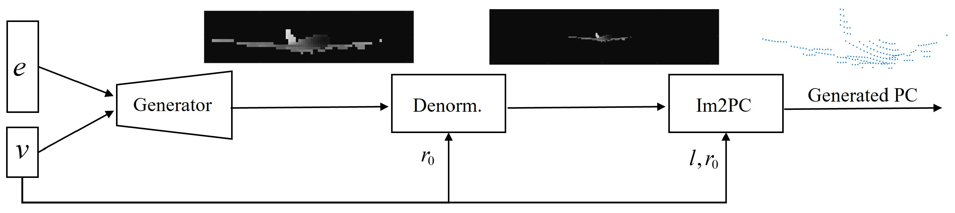
2.1. APCG Method
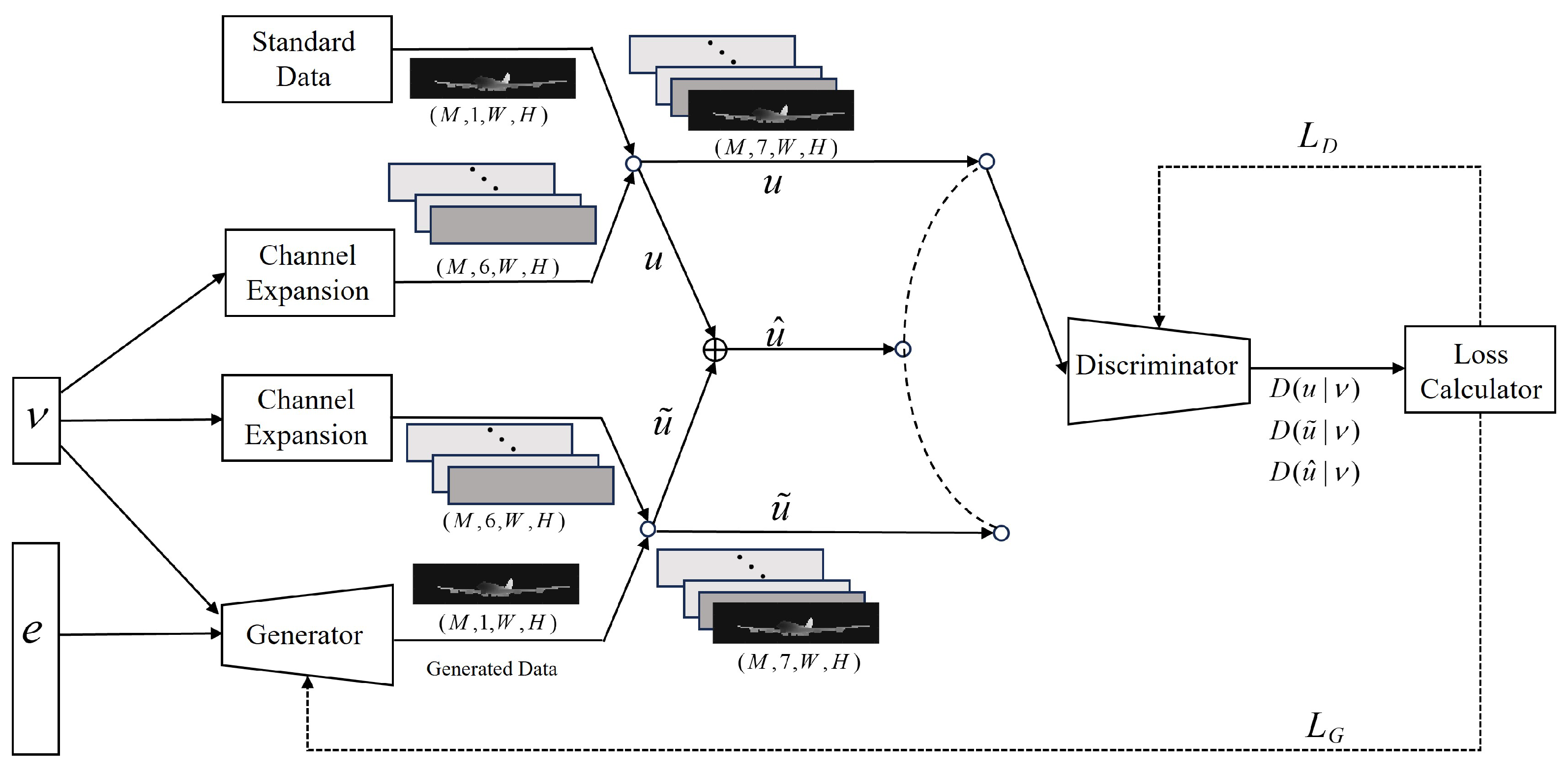
2.2. Improved cGAN
2.2.1. Improved cGAN Based on Depth Image
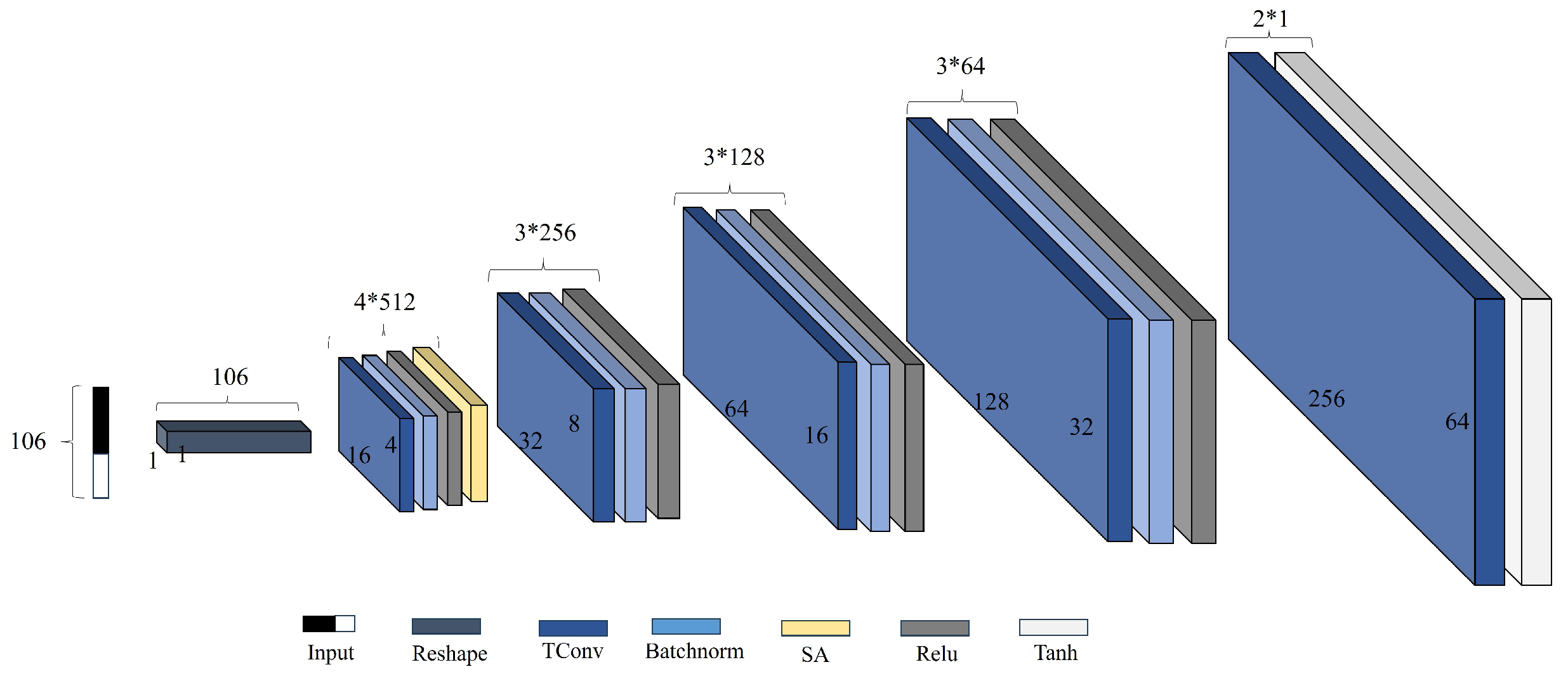
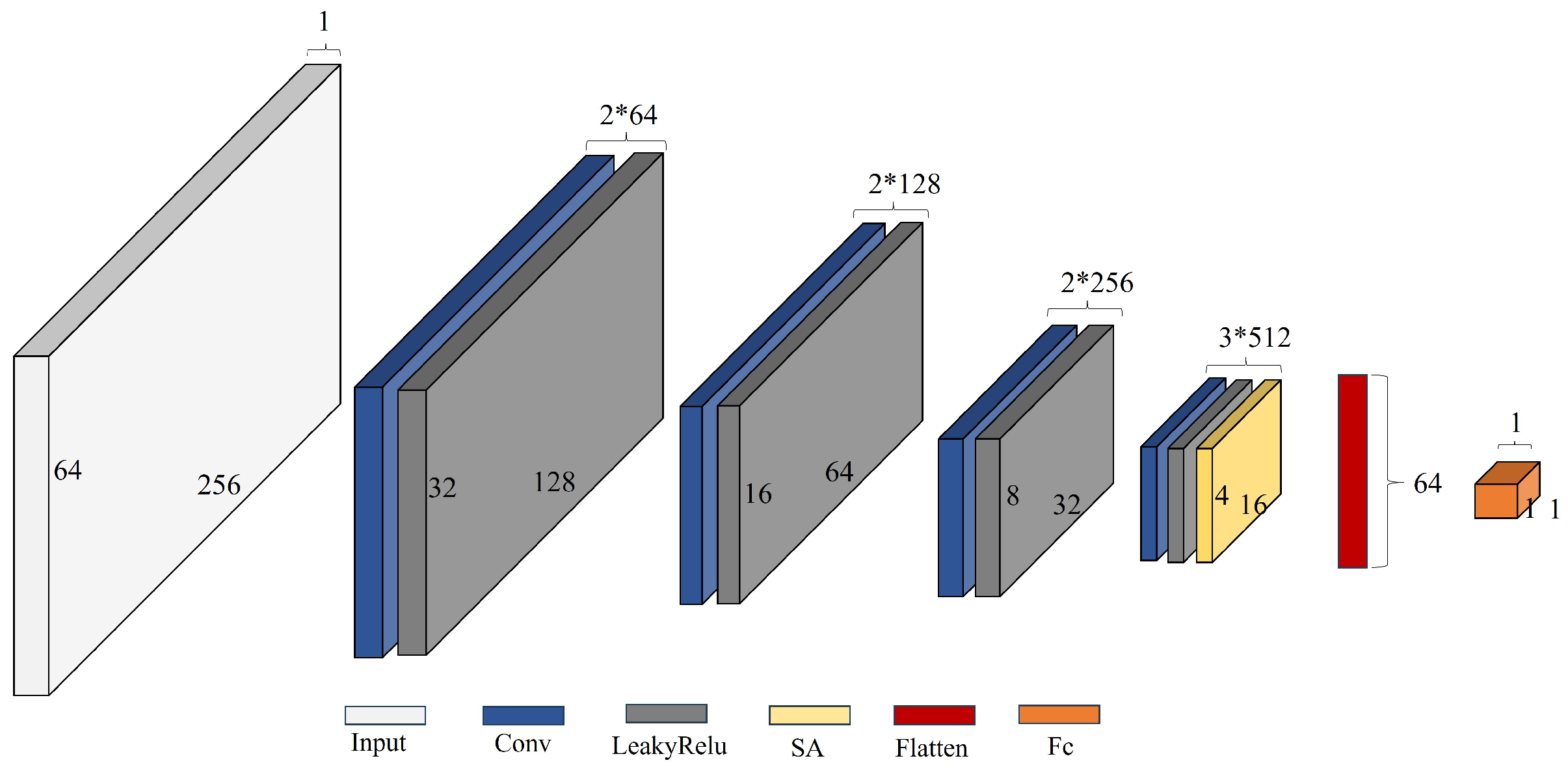
2.2.2. Generator of Improved cGAN
2.2.3. Discriminator of Improved cGAN
2.2.4. Training Process
2.3. Standard Data Generator
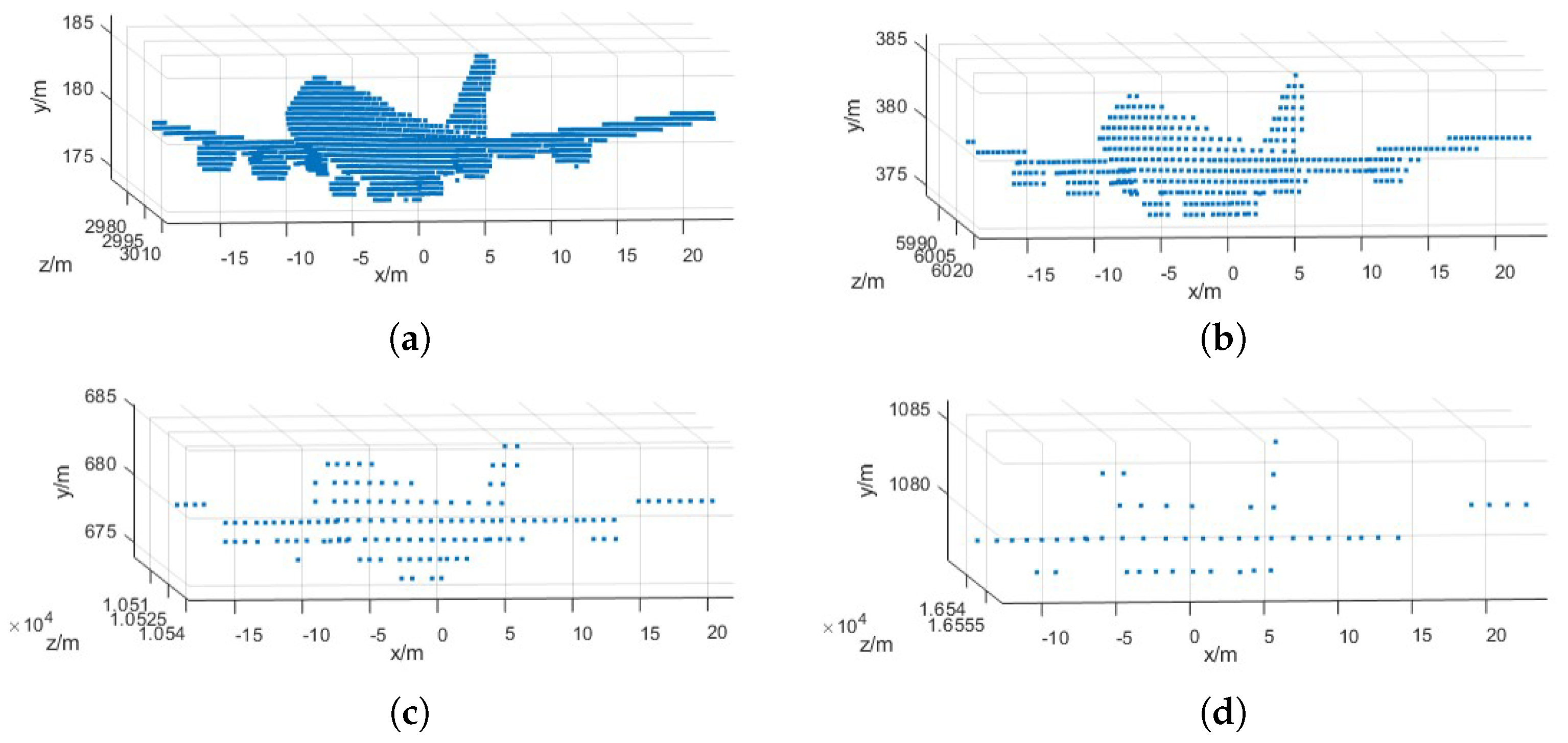
2.3.1. Parameter Selection of SPC-Lidar
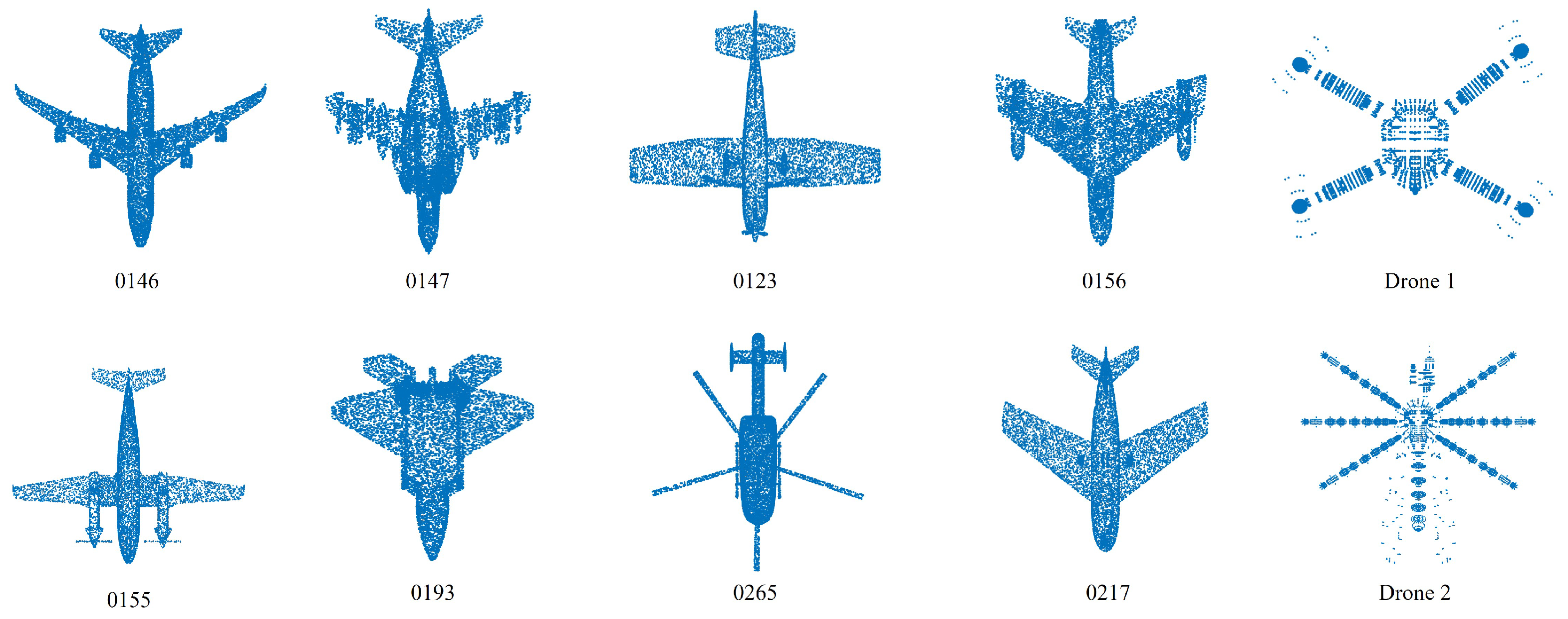
2.3.2. Simulation of Standard Point Cloud Data of Aircraft
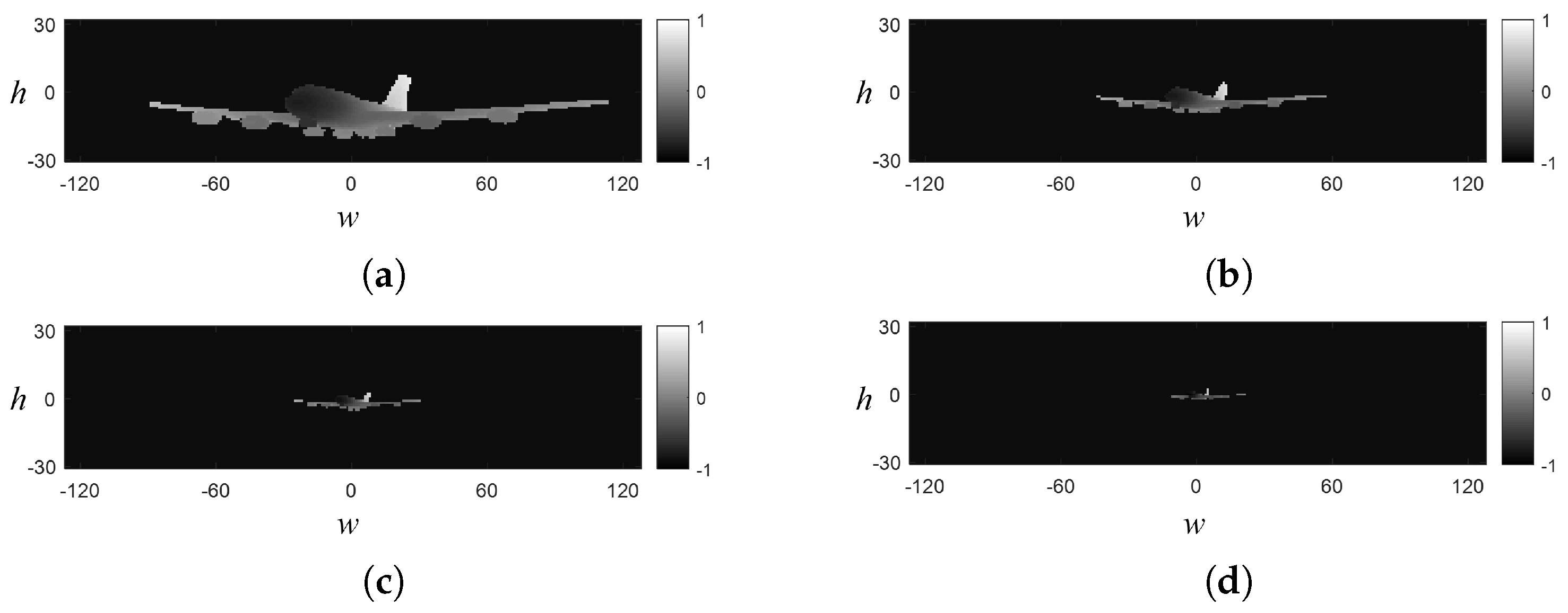
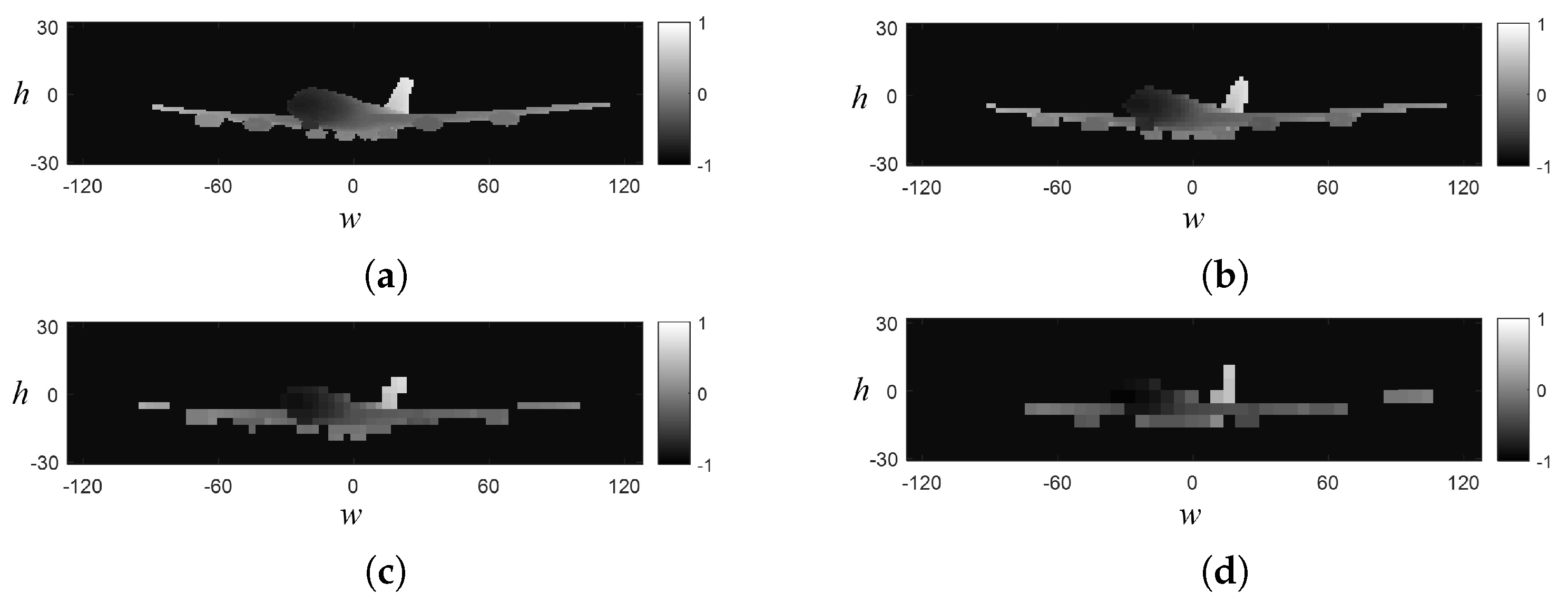
2.3.3. Generation of Depth Image
2.3.4. Normalization of Target Pixel Occupancy
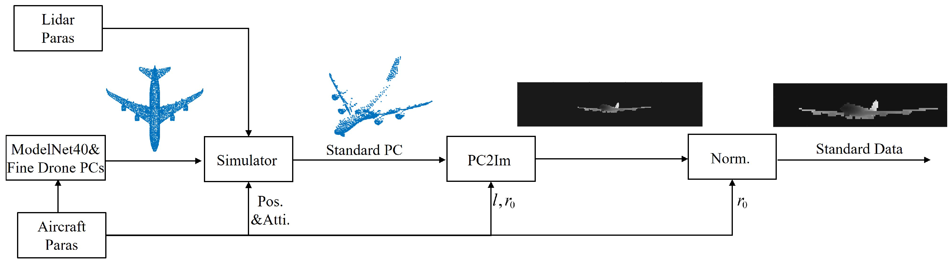
2.3.5. Aircraft Standard Data Generator
3. Experimental Results
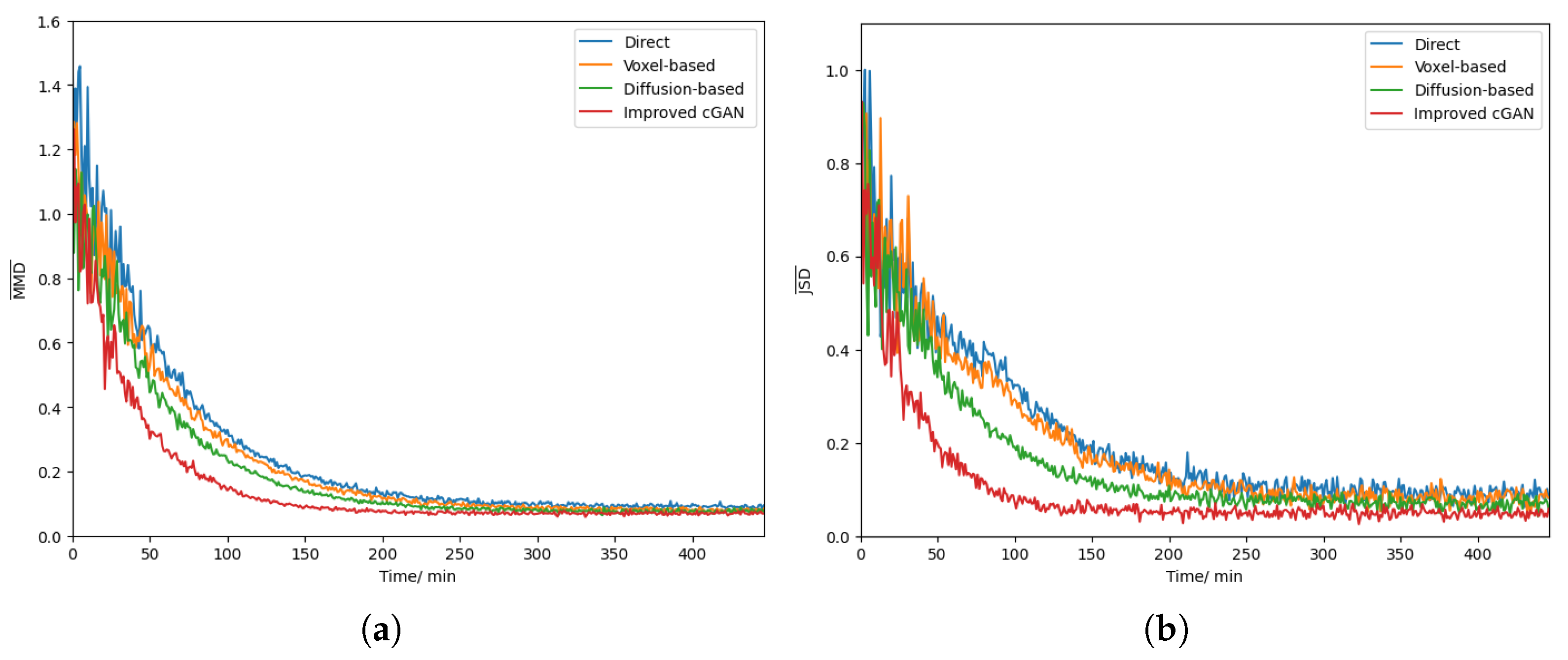
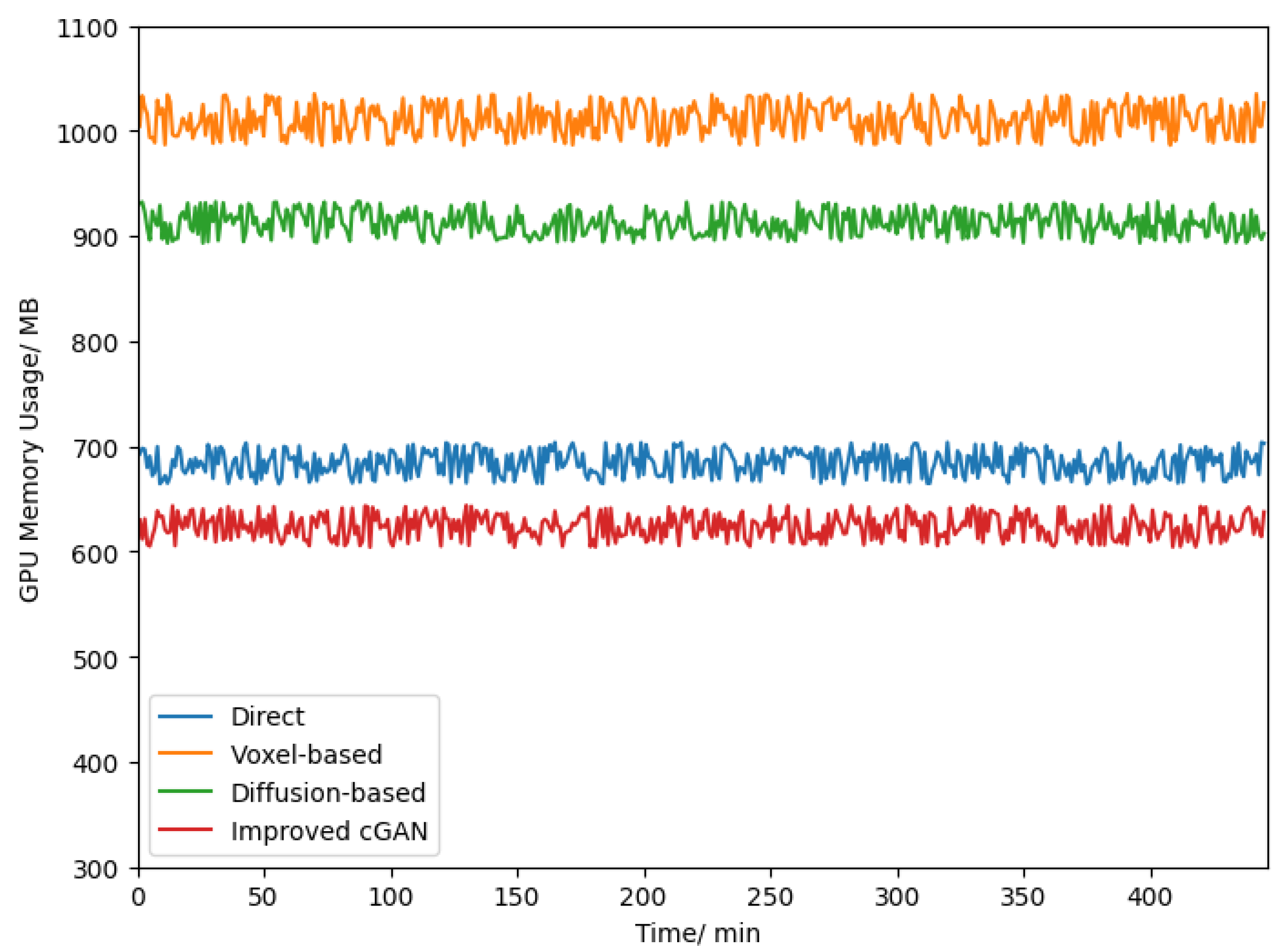
3.1. Training of Improved cGAN
3.2. Ablation Experiment on Improved cGAN
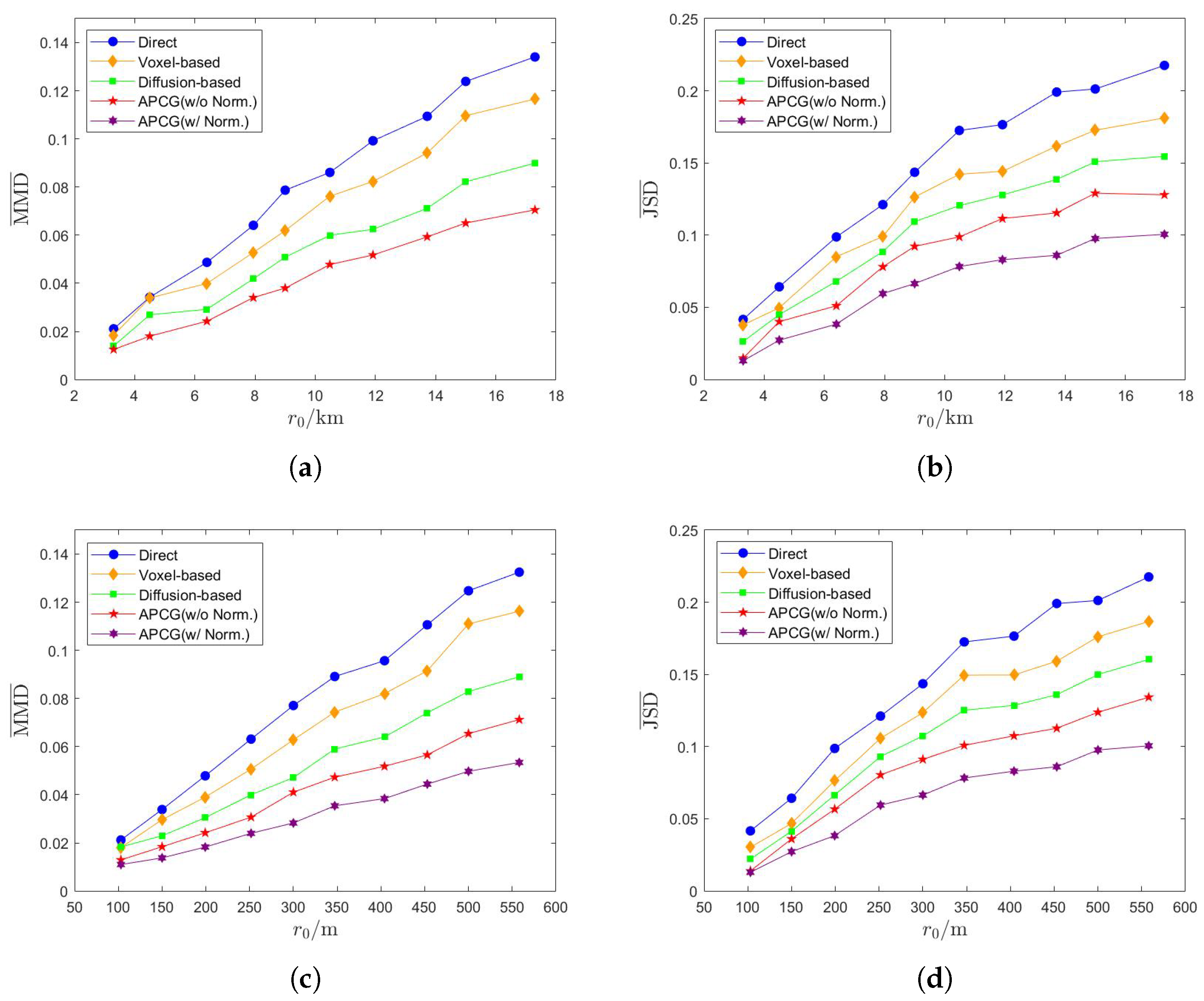
3.3. Performance of APCG
4. Discussion
- 1.
- The improved cGAN possesses superior generalization ability. Convolutional layers, transposed convolutional layers, and self-attention layers are introduced into the basic framework of the cGAN, and the loss function based on Wasserstein distance is adopted to replace the traditional loss function based on binary cross-entropy. The results of the ablation experiments indicate that these improvements all facilitate the enhancement of the quality and diversity of the images generated by the cGAN.
- 2.
- APCG possesses the capability of generating aircraft point clouds efficiently based on specific conditional information. APCG constructs an aircraft point cloud generation model with the aircraft depth image generator as the core. The aircraft depth image generator is the generator in the successfully trained improved cGAN, and the training data of this improved cGAN are the aircraft depth image data converted from the characteristics of the aircraft point clouds collected by the SPC-Lidar system. Hence, APCG can rapidly generate aircraft point clouds that conform to the collection characteristics of the SPC-Lidar system by utilizing the type, position, and attitude information of the aircraft.
5. Conclusions
Author Contributions
Funding
Institutional Review Board Statement
Informed Consent Statement
Data Availability Statement
Conflicts of Interest
Abbreviations
| APCG | Aircraft Point Cloud Generation |
| SPC | Single Photon Counting |
| cGAN | Conditional Generative Adversarial Network |
| GAN | Generative Adversarial Network |
| FPD | Frechet Point Cloud Distance |
| MMD | Maximum Mean Discrepancy |
| JSD | Jensen–Shannon Divergence |
| KL | Kullback–Leibler |
| FID | Frechet Inception Distance |
| GPU | Graphic Processing Unit |
| SA | Self-Attention |
| FC | Fully Connected |
Appendix A. Average Values of MMD and JSD
Appendix A.1. Average Value of MMD
Appendix A.2. Average Value of JSD
References
- Chu, T.; Wang, L. Research on Flight Safety Assessment Method of UAV in Low Altitude Airspace. In Proceedings of the International Conference on Autonomous Unmanned Systems, Singapore, 23 September 2022; pp. 1299–1307. [Google Scholar]
- Rapp, J.; Tachella, J.; Altmann, Y.; McLaughlin, S.; Goyal, V.K. Advances in single-photon lidar for autonomous vehicles: Working principles, challenges, and recent advances. IEEE Signal Process. Mag. 2020, 37, 62–71. [Google Scholar] [CrossRef]
- Popescu, S.C.; Zhou, T.; Nelson, R.; Neuenschwander, A.; Sheridan, R.; Narine, L.; Walsh, K.M. Photon counting LiDAR: An adaptive ground and canopy height retrieval algorithm for ICESat-2 data. Remote Sens. Environ. 2018, 208, 154–170. [Google Scholar] [CrossRef]
- Ma, Y.; Zhang, W.; Li, S.; Cui, T.; Li, G.; Yang, F. A new wind speed retrieval method for an ocean surface using the waveform width of a laser altimeter. Can. J. Remote Sens. 2017, 43, 309–317. [Google Scholar] [CrossRef]
- Wang, Z.; Menenti, M. Challenges and opportunities in Lidar remote sensing. Front. Remote Sens. 2021, 2, 641723. [Google Scholar] [CrossRef]
- Wald, I.; Woop, S.; Benthin, C.; Johnson, G.S.; Ernst, M. Embree: A kernel framework for efficient CPU ray tracing. ACM Trans. Graph. 2014, 33, 143. [Google Scholar] [CrossRef]
- Su, Z.; Sang, L.; Hao, J.; Han, B.; Wang, Y.; Ge, P. Research on Ground Object Echo Simulation of Avian Lidar. Photonics 2024, 11, 153. [Google Scholar] [CrossRef]
- Laine, S.; Karras, T. Efficient Sparse Voxel Octrees—Analysis, Extensions, and Implementation; NVIDIA Corporation: Santa Clara, CA, USA, 2010; Volume 2. [Google Scholar]
- Choi, S.; Zhou, Q.Y.; Koltun, V. Robust reconstruction of indoor scenes. In Proceedings of the IEEE Conference on Computer Vision and Pattern Recognition, Boston, MA, USA, 7–12 June 2015; pp. 5556–5565. [Google Scholar]
- Macklin, M.; Müller, M.; Chentanez, N.; Kim, T.Y. Unified particle physics for real-time applications. ACM Trans. Graph. 2014, 33, 153. [Google Scholar] [CrossRef]
- Koschier, D.; Bender, J.; Solenthaler, B.; Teschner, M. A survey on SPH methods in computer graphics. Comput. Graph. Forum. 2022, 41, 737–760. [Google Scholar] [CrossRef]
- Goodfellow, I.; Pouget-Abadie, J.; Mirza, M.; Xu, B.; Warde-Farley, D.; Ozair, S.; Courville, A.; Bengio, Y. Generative adversarial nets. Adv. Neural Inf. Process. Syst. 2014, 27, 2672–2680. [Google Scholar]
- Zhou, Y.; Tuzel, O. VoxelNet: End-to-end learning for point cloud-based 3D object detection. In Proceedings of the IEEE Conference on Computer Vision and Pattern Recognition, Salt Lake City, UT, USA, 18–22 June 2018; pp. 4490–4499. [Google Scholar]
- Wang, X.; Ang, M.H.; Lee, G.H. Voxel-based network for shape completion by leveraging edge generation. In Proceedings of the IEEE/CVF International Conference on Computer Vision, Montreal, QC, Canada, 10–17 October 2021; pp. 13189–13198. [Google Scholar]
- Achlioptas, P.; Diamanti, O.; Mitliagkas, I.; Guibas, L. Learning representations and generative models for 3D point clouds. In Proceedings of the International Conference on Machine Learning, PMLR, Stockholm, Sweden, 10–15 July 2018; pp. 40–49. [Google Scholar]
- Shu, D.W.; Park, S.W.; Kwon, J. 3D point cloud generative adversarial network based on tree-structured graph convolutions. In Proceedings of the IEEE/CVF International Conference on Computer Vision, Seoul, Republic of Korea, 27 October–2 November 2019; pp. 3859–3868. [Google Scholar]
- Fan, H.; Su, H.; Guibas, L.J. A point set generation network for 3D object reconstruction from a single image. In Proceedings of the IEEE Conference on Computer Vision and Pattern Recognition, Honolulu, HI, USA, 21–26 July 2017; pp. 605–613. [Google Scholar]
- Mandikal, P.; Navaneet, K.L.; Agarwal, M.; Babu, R.V. 3D-LMNet: Latent embedding matching for accurate and diverse 3D point cloud reconstruction from a single image. In Proceedings of the British Machine Vision, Newcastle upon Tyne, UK, 3–6 September 2018; pp. 3–6. [Google Scholar]
- Zyrianov, V.; Zhu, X.; Wang, S. Learning to generate realistic lidar point clouds. In Proceedings of the European Conference on Computer Vision, Tel Aviv, Israel, 23–27 October 2022; pp. 17–35. [Google Scholar]
- Zhang, J.; Zhang, F.; Kuang, S.; Zhang, L. Nerf-lidar: Generating realistic lidar point clouds with neural radiance fields. In Proceedings of the AAAI Conference on Artificial Intelligence, Vancouver, BC, Canada, 7–14 February 2024; pp. 7178–7186. [Google Scholar]
- Mirza, M. Conditional generative adversarial nets. arXiv 2014, arXiv:1411.1784. [Google Scholar]
- Radford, A. Unsupervised representation learning with deep convolutional generative adversarial networks. arXiv 2015, arXiv:1511.06434. [Google Scholar]
- Zhang, H.; Goodfellow, I.; Metaxas, D.; Odena, A. Self-attention generative adversarial networks. In Proceedings of the International Conference on Machine Learning, Long Beach, CA, USA, 9–15 June 2019; pp. 7354–7363. [Google Scholar]
- Gulrajani, I.; Ahmed, F.; Arjovsky, M.; Dumoulin, V.; Courville, A.C. Improved training of Wasserstein GANs. Adv. Neural Inf. Process. Syst. 2017, 30, 5769–5779. [Google Scholar]
- Wu, Z.; Song, S.; Khosla, A.; Yu, F.; Zhang, L.; Tang, X.; Xiao, J. 3D ShapeNets: A deep representation for volumetric shapes. In Proceedings of the IEEE Conference on Computer Vision and Pattern Recognition, Boston, MA, USA, 7–12 June 2015; pp. 1912–1920. [Google Scholar]
- Heusel, M.; Ramsauer, H.; Unterthiner, T.; Nessler, B.; Hochreiter, S. GANs trained by a two time-scale update rule converge to a local Nash equilibrium. Adv. Neural Inf. Process. Syst. 2017, 30, 6629–6640. [Google Scholar]
- Luo, S.; Hu, W. Diffusion probabilistic models for 3d point cloud generation. In Proceedings of the IEEE/CVF Conference on Computer Vision and Pattern Recognition, Nashville, TN, USA, 19–25 June 2021; pp. 2837–2845. [Google Scholar]


| Parameter | Number | Range |
|---|---|---|
| 5 | ||
| 10 | for aircraft | |
| for drone | ||
| 10 | ||
| 5 | ||
| 5 |
| Parameter | Value |
|---|---|
| Decay rate for first moment estimate | 0.5 |
| Decay rate for second moment estimate | 0.9 |
| Learning rate of generator | |
| Learning rate of discriminator | |
| Total number of training epochs | 1000 |
| Batch size | 32 |
| cGAN | FID | ||
|---|---|---|---|
| TConv/Conv | SA | Wasserstein Loss | |
| — | — | — | 52.6 |
| ✓ | — | — | 45.6 |
| — | ✓ | — | 48.4 |
| — | — | ✓ | 46.7 |
| ✓ | ✓ | — | 41.9 |
| — | ✓ | ✓ | 44.0 |
| ✓ | — | ✓ | 44.8 |
| ✓ | ✓ | ✓ | 40.6 |
Disclaimer/Publisher’s Note: The statements, opinions and data contained in all publications are solely those of the individual author(s) and contributor(s) and not of MDPI and/or the editor(s). MDPI and/or the editor(s) disclaim responsibility for any injury to people or property resulting from any ideas, methods, instructions or products referred to in the content. |
© 2025 by the authors. Licensee MDPI, Basel, Switzerland. This article is an open access article distributed under the terms and conditions of the Creative Commons Attribution (CC BY) license (https://creativecommons.org/licenses/by/4.0/).
Share and Cite
Su, Z.; Liang, S.; Hao, J.; Han, B. Research on Low-Altitude Aircraft Point Cloud Generation Method Using Single Photon Counting Lidar. Photonics 2025, 12, 205. https://doi.org/10.3390/photonics12030205
Su Z, Liang S, Hao J, Han B. Research on Low-Altitude Aircraft Point Cloud Generation Method Using Single Photon Counting Lidar. Photonics. 2025; 12(3):205. https://doi.org/10.3390/photonics12030205
Chicago/Turabian StyleSu, Zhigang, Shaorui Liang, Jingtang Hao, and Bing Han. 2025. "Research on Low-Altitude Aircraft Point Cloud Generation Method Using Single Photon Counting Lidar" Photonics 12, no. 3: 205. https://doi.org/10.3390/photonics12030205
APA StyleSu, Z., Liang, S., Hao, J., & Han, B. (2025). Research on Low-Altitude Aircraft Point Cloud Generation Method Using Single Photon Counting Lidar. Photonics, 12(3), 205. https://doi.org/10.3390/photonics12030205