Decoding Anomalous Diffusion Using Higher-Order Spectral Analysis and Multiple Signal Classification

Abstract

Anomalous diffusion is characterized by nonlinear growth in the mean square displacement of a trajectory. Recent advances using statistical methods and recurrent neural networks have made it possible to detect such phenomena, even in noisy conditions. In this work, we explore feature extraction through parametric and non-parametric spectral analysis methods to decode anomalously diffusing trajectories, achieving reduced computational costs compared with other approaches that require additional data or prior training. Specifically, we propose the use of higher-order statistics, such as the bispectrum, and a hybrid algorithm that combines kurtosis with a multiple-signal classification technique. Our results demonstrate that the type of trajectory can be identified based on amplitude and kurtosis values. The proposed methods deliver accurate results, even with short trajectories and in the presence of noise.

1. Introduction

Anomalous diffusion appears in many physical, chemical, biological, and human phenomena. Examples include molecular encounters in reactions [1,2,3], cellular signaling [4,5], the foraging of animals [6,7,8] the spread of diseases [9], and trends in financial markets and climate records. In disordered photonic systems, we can find examples in which light propagation exhibits a subdiffusive behavior [10]. This is the case when photons remain trapped for longer periods due to multiple scattering events, but we can also find examples of superdiffusive behavior, where photons propagate more rapidly due to collective phenomena or localized excitations [11].

Deviations from Brownian diffusion, known as anomalous diffusion (AnDi), occur when the mean square displacement (MSD) growth with time has an exponent other than one. The classic example of AnDi is Brownian motion, which describes the motion of a microscopic particle in a fluid as a consequence of thermal forces [12,13].

Several methods have been used in the classification of anomalous diffusion trajectories. Lately, neural networks have been the most widely used method as they can efficiently characterize the anomalous diffusion by determining the exponent of a single short path exceeding the standard estimate based on MSD when the available data are limited, as is often the case in experiments [14,15,16,17,18,19,20].

Recent advancements in machine learning, specifically in deep learning and neural networks, have demonstrated considerable success in analyzing complex patterns and predicting events in noisy data environments [21,22]. Recurrent neural networks (RNNs), in particular, have shown promise for identifying temporal dependencies and sequential patterns, which are essential for characterizing anomalous diffusion processes [23,24]. The integration of statistical methods with RNNs has enabled the development of robust frameworks that can detect and predict the occurrence of anomalous diffusion, even in the presence of significant noise [25,26]. This approach aligns with recent works in the field of deep learning, where neural networks are increasingly applied to complex, non-linear systems to uncover underlying behaviors and trends [21,22]. By leveraging these techniques, we aim to improve accuracy for identifying diffusion types without the need for extensive preprocessing or noise filtering. This paper, therefore, contributes to the broader application of a combination of higher-order statistics and artificial intelligence in analyzing and predicting phenomena within stochastic and noisy environments, positioning our work within the current trend of using deep learning to solve complex analytical challenges.

Regarding other classification methods, several works use spectral analysis [27,28,29], where criteria based on the power spectrum are used for Fractional Brownian Motion (FBM) trajectories and other related work using Bayesian inference [30,31,32].

Some works have been conducted using moving displacement arithmetic based on first and second-order statistics, such as the mean value and the variance to analyze anomalous diffusion [33], as well as in specific applications, such as to characterize the random movement patterns of animals [34], and in the classification of particle trajectories in living cells [35].

Although a punctual classification of the studied sequence is obtained with the above methods, they are not immune to interference. In processes where noise is also present, good results are not obtained. In general, using estimators [36] that do not involve prior information about the data, such as prior training, can speed up the computational process as these methods only depend on a successful non-linear combination that identifies the analyzed processes.

Parametric and non-parametric high-resolution spectral analysis can effectively analyze anomalous diffusion as an estimator of the characteristics and descriptive patterns that random trajectories may present, differentiating the helpful information from noise within the anomalous diffusion series. The use of high-order spectral analysis provides certain advantages over classical processing methods like power spectrum because the statistics of random processes of orders greater than two are theoretically zero [37,38], as well as over high-resolution spectral analysis [39,40], which is based on the calculation of the spectrum using the vector subspaces of the eigenvalue matrix of the information to be analyzed [41,42].

In this work, we propose a non-parametric estimation approach using the signal bispectrum in combination with first-order statistics, such as the mean value, to characterize anomalous diffusion sequences. We also propose combining high-resolution spectral analysis with fourth-order statistics such as kurtosis to decode anomalous diffusion trajectories for a reduced data set. By now, our methods cannot yet be compared with the huge data sets used for training the most successful methods in the Andi Challenge. In this regard, we have focused on presenting an alternative perspective for studying anomalous diffusion using signal analysis tools and a more understandable interpretation of these models’ behavior.

The trajectories used in the experiments presented in this work follow one of these five types of anomalous diffusion [43,44]: Annealed Transit Time Model (ATTM), Continuous Time Random Walk (CTRW), Fractional Brownian Motion (FBM), Lévy Walk (LW), and Scaled Brownian Motion (SBM).

The paper is organized as follows. Section 2 provides a brief theoretical description of the fundamentals of anomalous diffusion involving each trajectory. Section 3 provides the theoretical foundations that support the analysis based on higher-order spectra, and Section 4 shows the experimental description of each trajectory. Section 5 describes the obtained results using the first proposed method based on the mean value of the bispectrum. Section 6 describes the results using the analysis of the proposed hybrid algorithm based on multiple signal classification and kurtosis. Finally, we discuss the results in Section 7 and show the conclusions in Section 8.

2. Fundamentals of Anomalous Diffusion

The process that gives rise to diffusion is stochastic or random, clearly illustrated by the paradigmatic example of Brownian motion. This motion consists of the irregular and unpredictable displacement of small particles suspended on the surface of a fluid and was explained in [45,46]. Unlike a normal diffusion process, in which the squared displacement is a linear function of time, anomalous diffusion is a diffusion process that involves a non-linear relationship between the mean square displacement (MSD) ${\sigma }_r^2$ and time t [47]. That is, the probability $P(x,t)$ of encountering a particle at time t and position x is described using a power law ${\sigma }_r^2\sim D{t}^{\alpha }$ where D is the diffusion coefficient. There are several models and derivations of anomalous diffusion trajectories. The following is a theoretical description of the models discussed in this work.

2.1. Annealed Transit Time Model (ATTM)

In this model, the initial point of the trajectory starts at $x=0$ for $t=0$, and we follow Langevin’s equation [48] at several instances. The random motion of the particle diffuses with a coefficient $D_1$ for a time ${\tau }_1$. Then, successive pairs are generated in the form $\left[D_n,{\tau }_n\right]$. The length of the interval ${\tau }_n$ varies with $D_n$, such that the Probabilistic Density Function (PDF) has a mean of $E[{\tau }_n,D_n]=D^{-\gamma }$. For $\gamma >0$, we expect to find larger periods of low dispersal Brownian motion combined with shorter periods of high dispersal [49,50].

2.2. Continuous Time Random Walk (CTRW)

The CTRW model is a generalization of the classical random walk, where a particle can be described as a sequence of movements sampled from a Gaussian distribution with zero mean. Besides, there are also waiting times between displacements that are sampled from a power-law distribution $\Psi \left(t\right)=t^{-\sigma }$. This long waiting time can lead to anomalous diffusion [51].

2.3. Fractional Brownian Motion (FBM)

FBM is a generalization of classical Brownian motion in which the jumps are not independent. FBM is a continuous-time Gaussian process $B_H\left(t\right)$ defined on $[0,T]$, with $E\left[B_H\left(t\right)\right]=0$ for all $t\ge 0$, and a covariance function given by [52]:

$$E\left[B_H\left(t\right)B_H\left(s\right)\right]={\displaystyle \frac{1}{2}}\left[{\left|t\right|}^{2H}+{\left|s\right|}^{2H}-{|t-s|}^{2H}\right]$$

(1)

where H is the Hurst exponent, $0\le H\le 1$. If $H={\displaystyle \frac{1}{2}}$, the process reduces to standard Brownian motion. For $H>{\displaystyle \frac{1}{2}}$, increments are positively correlated (superdiffusion), while for $H<{\displaystyle \frac{1}{2}}$, increments are negatively correlated (subdifussion), see [53,54].

2.4. Lévy Walk (LW)

Lévy walks (LWs) are a particular case of CTRW where dispersal lengths correlate with waiting times. The PDF describing random time intervals between consecutive jumps is a power-law function $\psi \left(t\right)=t^{-\sigma -1}$ (as in the CTRW). Besides, the probability of a $\Delta x$ dispersal length is given by $\Psi (\Delta x,t)={\displaystyle \frac{1}{2}}\delta \left(\right|\Delta x)-vt)\psi \left(t\right)$ [44,55,56].

2.5. Scaled Brownian Motion: SBM

This model is derived from the Langevin equation. However, here, the diffusivity changes with time, even in the Gaussian noise case [57,58,59].

3. Higher-Order Spectral Analysis: Bispectrum

After briefly showing the theoretical background of the anomalous diffusion trajectories, let us briefly introduce the higher-order spectral analysis. The bispectrum is defined as the Fourier Transform of the third-order cumulant, which is given by (2):

$$B(f_1,f_2)=\sum _{{\tau }_1=-N+1}^{N-1}\sum _{{\tau }_2=-N+1}^{N-1}{C}_{3x}({\tau }_1,{\tau }_2)·e^{-2\pi f_1{\tau }_1}·e^{-2\pi f_2{\tau }_2}={\displaystyle \frac{1}{N^2}}X(f_1,f_2)·X\left(f_1\right)·X\left(f_2\right)$$

(2)

where $X\left(f\right)$ is the Fourier Transform of the sequence ${\left\{x\left(n\right)\right\}}_{n=0}^{N-1}$, $C_{3x}$ is the third-order cumulant of the input sequence, and sets $f_1$ and $f_2$ are integers from the matrix of bispectral frequencies obtained from the bispectrum calculation.

In the spectral domain, the bispectrum can also be computed through convolution in the spectral domains, as shown in (3). The convolution theorem for bispectrum analysis extends the principles of the Fourier transform to higher-order spectral analysis. Specifically, in the context of the bispectrum, which is a second-order frequency domain representation involving two frequency components, the theorem states that the bispectrum of the convolution of two signals in the time domain is equal to the product of their bispectra in the frequency domain.

$$B(f_1,f_2)=X(f_1+f_2)·X\left(f_1\right)·X\left(f_2\right)$$

(3)

We used the absolute value of the bispectrum signal as described in (4), which will be computed from (2), where N is the number of rows of the square matrix $N\times N$ obtained from the bispectrum. The obtained result is a complex $N\times N$ matrix that contains the frequency values of the amplitude bispectrum matrix of the data set.

$$B_a(f_1,f_2)={\left|B(f_1,f_2)\right|}_i\forall i=1,\dots ,N$$

(4)

Once Equation (4) has been obtained and in order to characterize each trajectory, in this work, we use an indicator based on the mean value of the bispectrum (Equation (5)), which is defined as follows:

$$M\left(B_a(f_1,f_2)\right)={\displaystyle \frac{1}{N}}\sum _{i=1}^N{B}_a(f_1,f_2).$$

(5)

3.1. Hybrid Algorithm: Multiple Signal Classification and Kurtosis

The proposed method is divided into two phases to ensure accurate frequency estimation and analysis. First, we obtain the pseudospectrum of the signal through the MUSIC algorithm, and then we calculate the bispectrum to capture non-linear interactions and phase coupling between different frequency components. This two-phase approach ensures that the method combines high-resolution frequency estimation (from the MUSIC algorithm) with a deeper analysis of the frequency interactions (from bispectral or higher-order techniques), leading to more robust and accurate signal analysis.

3.1.1. First Phase: Pseudospectrum Estimation Using the MUSIC Algorithm

In this phase, we apply the multiple signal classification (MUSIC) algorithm to estimate the pseudospectrum of a given trajectory using Schmidt’s eigenspace analysis method [60]. The MUSIC algorithm performs an eigenspace analysis of the data’s correlation matrix, separating the signal subspace from the noise subspace. The pseudospectrum $Pm\left(f\right)$, computed from the covariance of the eigenvalues of the data for each trajectory, is expressed as follows:

$$Pm\left(f\right)={\displaystyle \frac{1}{{\sum }_{k=1}^p\left(1-{\left|v_k^{H}e\left(f\right)\right|}^2\right)}}$$

(6)

where $v_k^H$ is the Hermitian transpose (or conjugate transpose) of the eigenvector $v_k$, and $e\left(f\right)$ is the steering vector corresponding to frequency f. Specifically:

• $v_k^H$ denotes the Hermitian transpose of the eigenvector $v_k$. This operation involves taking the transpose of the matrix and applying the complex conjugate to each element. It is used in signal processing to perform orthogonal analysis of the signal components.
• $e\left(f\right)$ represents the steering vector at frequency f, which describes the response of the system to a signal at that particular frequency. In the MUSIC algorithm, the steering vector helps evaluate how well the signal aligns with the subspace spanned by the eigenvectors.

The term ${\left|v_k^{H}e\left(f\right)\right|}^2$ represents the squared magnitude of the projection of the steering vector $e\left(f\right)$ onto the eigenvector $v_k$ and is used to determine the contribution of the signal in the corresponding eigenspace.

3.1.2. Second Phase: Bispectral Analysis

This phase enhances the frequency characterization by detecting phase relationships not captured by second-order methods like the MUSIC algorithm alone. We compute the bispectrum of the signal and then we evaluate the kurtosis to identify the trajectory patterns according to the following relation:

$$Pk={\displaystyle \frac{E\left(Pm\left(f\right)-{\upsilon }^4\right)}{{\sigma }^4}}$$

(7)

where $\upsilon$ and $\sigma$ are the mean and the standard deviation of $Pm\left(f\right)$, and E represents the expected value. This provides the characterization of each trajectory.

4. Experimental Description

We study five anomalous diffusion trajectory models: ATTM, CTRW, FBM, LW, and SBM. We have generated several trajectories using the same procedure as in [43,44]. Each trajectory has a standard deviation $\sigma$, with $0.5\le \sigma \le 1.0$; a variable exponent $\alpha$, with $0.1\le \alpha \le 0.9$; and a length of $2^N$, where $5\le N\le 10$.

The sequence length is chosen to be a power of two because it is advantageous for the computation of the bispectrum. This choice optimizes the computational efficiency, particularly when applying Fast Fourier Transforms (FFTs), which operate most efficiently when the length of the sequence is a power of two. As the bispectrum involves evaluating phase relationships between multiple frequencies, a sequence length that is a power of two ensures compatibility with FFT algorithms and enhances the precision of the frequency domain analysis. Additionally, using window lengths that are multiples of two for the bispectrum computation ensures uniform segmentation and avoids data loss at the edges of the windows. Figure 1 is an example of the bispectrum contour of an anomalous diffusion trajectory, in this case, for an ATTM sequence. As can be seen, a bispectral pattern can be unique for each sequence and can also be observed when identifying the characteristics in the trajectory analyzed.

The bispectrum results in a matrix containing the frequencies of the Fourier transform of the third-order cumulant of the data. The axes represent the bispectral content of each frequency in the harmonics that generate the anomalous diffusion sequence.

We briefly describe the data set of trajectories:

• For the ATTM and CTRW models, we considered 108 trajectories that represent the set of combinations of length, $2^N$ with $5\le N\le 10$, $\sigma =0.5,1$, and $\alpha =0.1,0.2,\dots ,0.9$.
• For the LW model, we considered 108 trajectories that represent the set of combinations of length, $2^N$ with $5\le N\le 10$, $\sigma =0.5,1$, and $\alpha =1.1,1.2,\dots ,1.9$.
• For the FBM and SBM models, we considered 210 trajectories that represent the set of combinations of length, $2^N$ with $5\le N\le 10$, $\sigma =0.5,1$, and $\alpha =0.05,\dots ,1.95$.

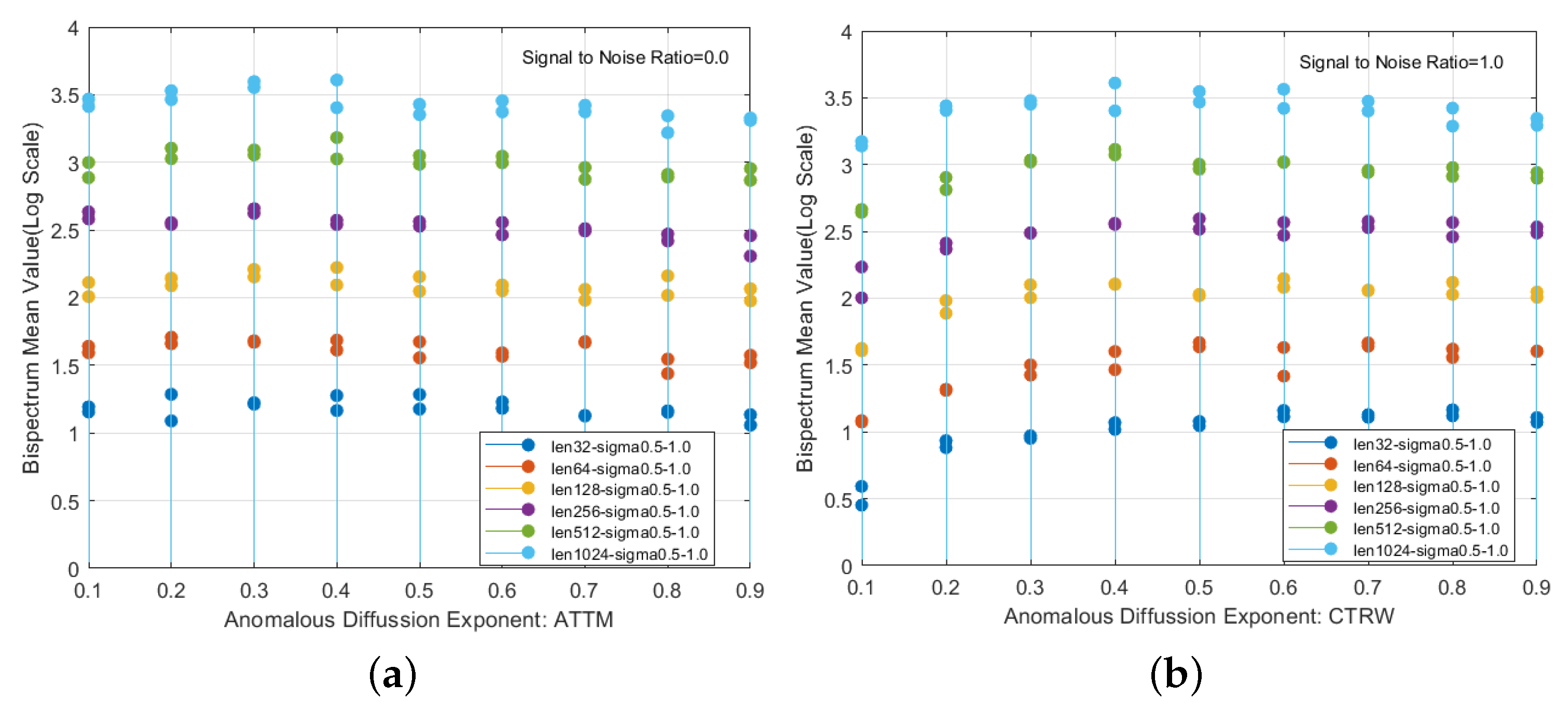
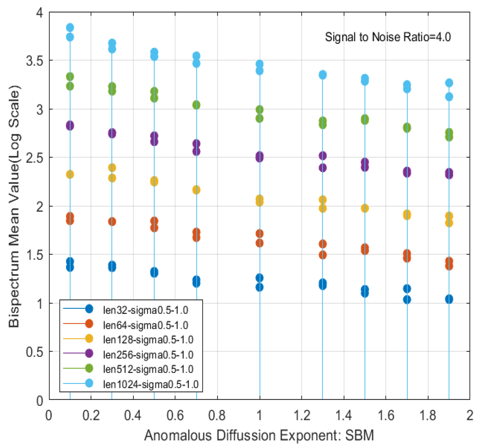
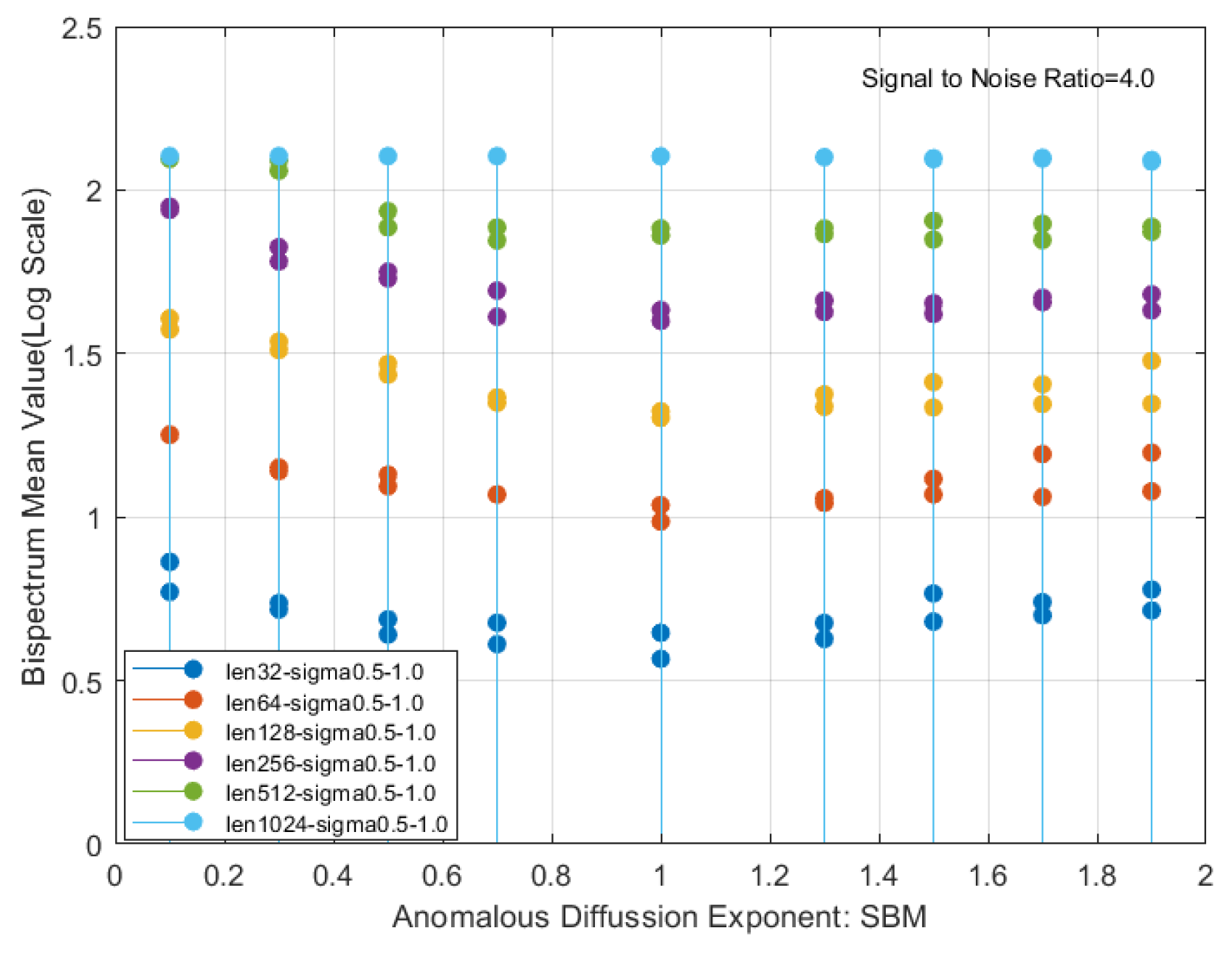
5. Results Based on the Mean Value of Bispectrum

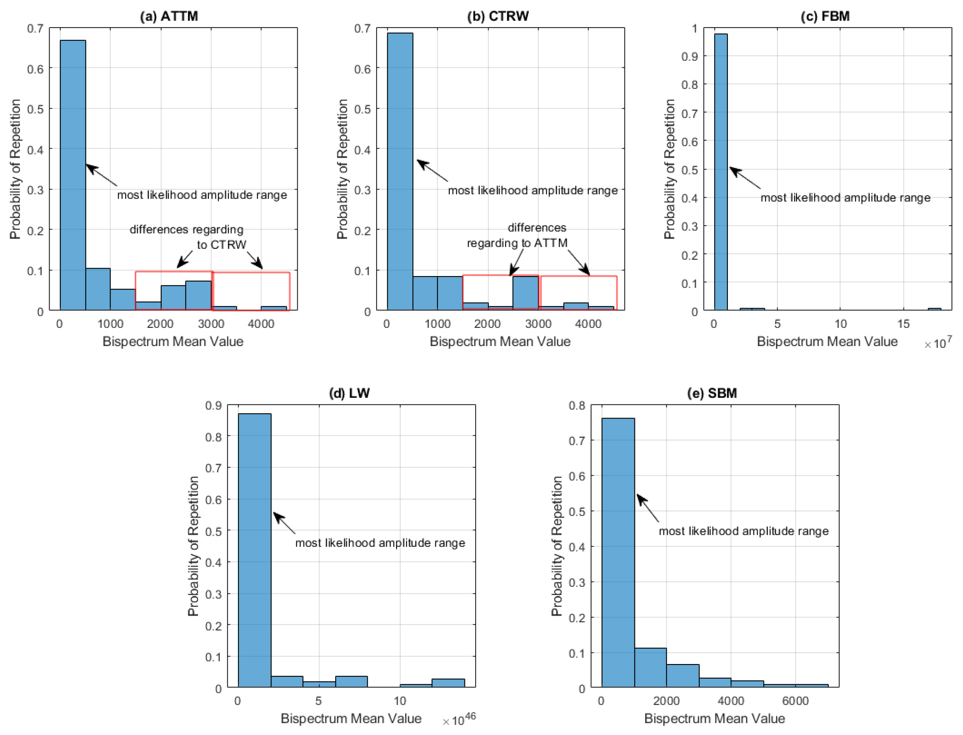
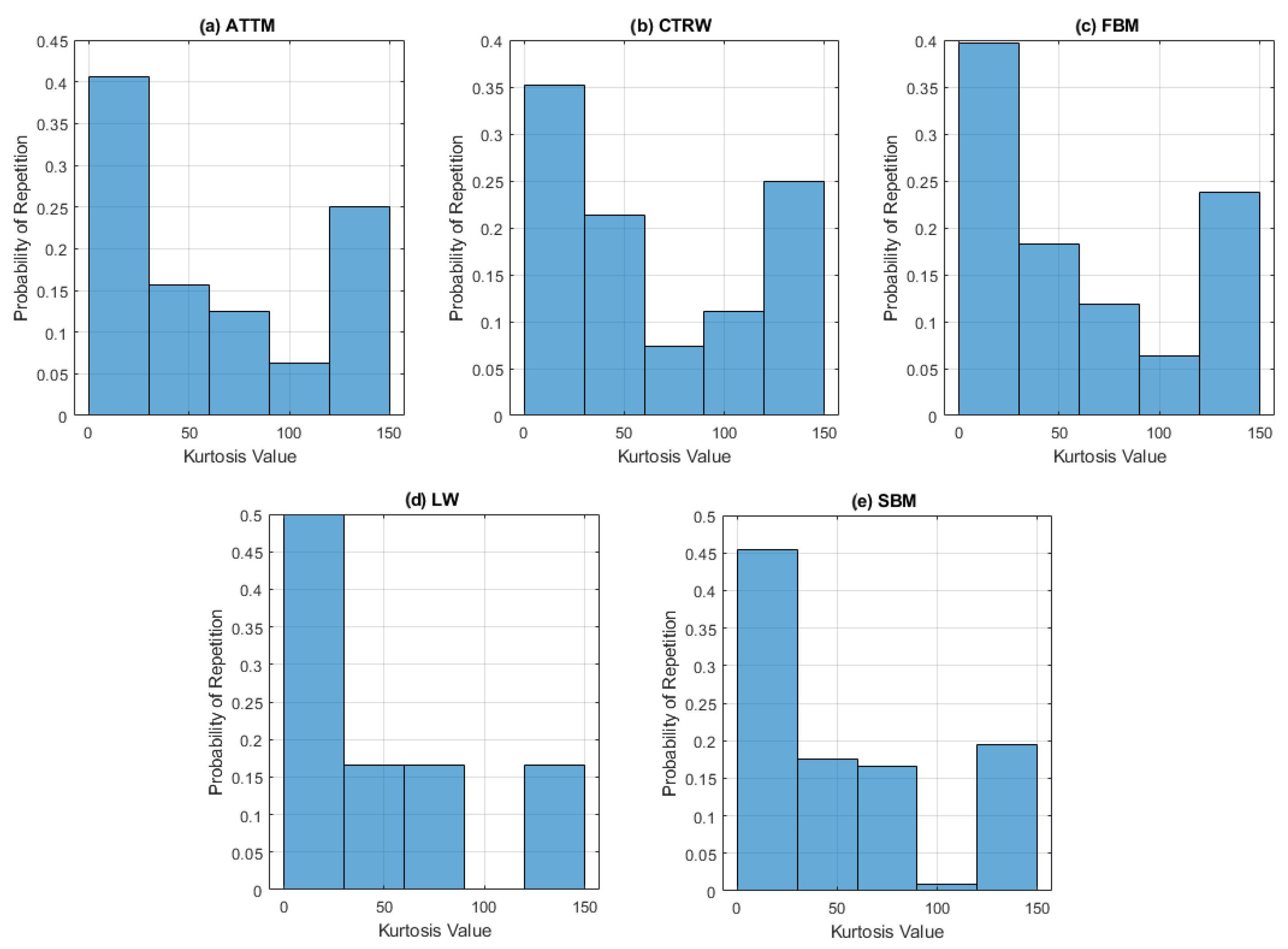
To obtain a classification method based on the previous results, we propose using methods based on first-order statistics combined with bispectrum analysis, see Equation (5). This classification type aims to characterize each trajectory so that each of the sequences studied can be quantitatively differentiated. Initially, the bispectrum of each sequence is taken as a basis for a specific trajectory, as aforementioned in Section 4.

Figure 2 shows the results obtained using the proposed indicator based on the bispectrum mean. For ATTM and CTRW trajectories, it can be seen that there are significant differences between the sequences for $\alpha \ge 0.2$, with the mean value increasing as long as the trajectory length does. There are no marked differences between the sequences of dimensions 32 and 64, respectively, whose mean value does not oscillate and remains almost unchanged over time.

It can also be seen in Figure 3 that the proposed algorithm can characterize the FBM trajectories. In this case, the result of the mean values of the bispectrum provides a representative curve as a function of the length of each sequence. In Figure 3, it can be noticed, analogous to Figure 2, that the average bispectrum value curve increases in amplitude as the sequence becomes longer, but with a more clear separation according to the sequence length. In the case of FBM, we see clear increasing trends depending on the length and the anomalous diffusion exponent. In contrast, LW shows a more homogeneous behavior for each sequence length, but with a wider separation between different lengths. Figure 4 shows the results obtained for SBM, which are closer to the ATTM model in the subdifussion regime. For SBM, the bispectrum’s mean values show a decreasing trend as the sequence length shortens, demonstrating a level of regularity not seen in LW trajectories.

Finally, in Figure 5, we show the overall behavior of the bispectral amplitude of the five analyzed models. It can be seen that the behavior of ATTM, CTRW, and SBM follows a similar trend, especially for the lowest lengths of 32, 64, and 12, increasing the amplitude as long as the trajectory length increases. This also happens for the FBM trajectory; the trend with the amplitude–length variation is also increasing, as we have already indicated, but mainly for long trajectories. Finally, the behavior of the LW trajectory is quite erratic and non-stationary, where no specific pattern can be distinguished, in contrast with the other cases.

Histogram Analysis

To decode each of the previously analyzed models in terms of the bispectrum and to evaluate how the amplitude is probabilistically distributed, we study the bispectrum amplitude probability histogram of each model to characterize each model. The obtained results are shown in Figure 6. We can see that all models have an asymmetric bispectrum probability distribution, and the highest amplitude probability is found at the lowest amplitudes. We also noticed that all models have different amplitude scale values as well as probability frequencies, except for the ATTM and CTRW trajectories, which have the same amplitude scale but slight differences.

To show the quantitative differences in the probability histograms of each type of trajectory, a correlation analysis is performed using Pearson’s coefficient. The obtained results are shown in

Table 1. Correlation matrix of the five trajectories used in the experiments.

	ATTM	CTRW	FBM	LW	SBM
ATTM	1	0	0	0	0
CTRW	0.7499	1	0	0	0
FBM	0.1016	0.1958	1	0	0
LW	−0.00616	−0.2267	−0.2390	1	0
SBM	−0.2261	0.1144	0.8255	0.7841	1

, where it is possible to appreciate the coherence of the correlation values with the similarities described above for the ATTM and CTRW sequences, respectively. Likewise, significant correlation values are also observed in the FBM–SBM and LW–SBM pairs, respectively, although the differences in the amplitude scale between the FBM, LW, and SBM trajectories are remarkable. This makes it easy to differentiate between the type of trajectory.

6. Results Using the Hybrid Algorithm: Multiple Signal Classification and Kurtosis

This section shows the results using a high-resolution spectral analysis method based on the covariance data matrix eigenvalues decomposition, in combination with a fourth-order statistic such as kurtosis, to achieve the identification of each model. The method reduces the computational cost and enhances noise immunity by combining two non-parametric estimators where the noise is zero. The proposed method is evaluated for each of the analyzed sequences. The results are shown in Figure 7.

In Figure 7, Figure 8 and Figure 9, it can be seen that the same pattern is obtained using the mean value of the bispectrum of each sequence. In this case, the kurtosis value of each trajectory decreases as the length of the sequence decreases. On the one hand, in all cases, it is possible to visualize with greater clarity the pattern of the short-length sequences 32–64 and 128, respectively. Likewise, the pattern of the LW trajectory is better defined. On the other hand, Figure 10 shows the results of the behavior of the kurtosis obtained from Equation (7) for each of the analyzed trajectories.

An upward-trending behavior in amplitude can be noticed as the sequence length increases. It can also be observed in all cases that the kurtosis of the sequence of length 1024 remains constant along the trajectory, with zero slope, except in the case of the SBM model. This feature identifies this model’s respect for others.

The histogram for each of the trajectories was also obtained. Figure 11 shows the obtained results, and in

Table 2. Correlation matrix of the five trajectories used in the experiments: MUSIC–kurtosis algorithm.

	ATTM	CTRW	FBM	LW	SBM
ATTM	1	0	0	0	0
CTRW	0.8860	1	0	0	0
FBM	0.5676	0.6199	1	0	0
LW	0.5327	0.8880	0.8432	1	0
SBM	0.9426	0.5144	0.9553	0.8566	1

we show the correlation matrix for each model, where it can be seen that there are no notable differences in each of the histograms, given that all the correlation values are greater than $0.5$.

Likewise, there is no discernible pattern of asymmetry in each distribution that could differentiate each trajectory.

7. Discussion

Having obtained the experimental results of the two analysis proposals to identify the anomalous diffusion trajectories, it can be said that:

• With the use of both the bispectrum-based method and the method using multiple signal classification and kurtosis, it is possible to identify each of the anomalous diffusion trajectories analyzed.
• The method based on multiple signal classification and kurtosis gives better results than the method based on the mean value of the bispectrum in the task of differentiating the type of trajectory according to its sequence length.
• With the bispectrum-based method, better results are obtained to identify the type of trajectory based on the probability histogram or the distribution of the amplitude values. As a quantitative indicator of this, the obtained results from the correlation matrix in both cases are shown.
• The average amplitude values of the bispectrum follow an asymmetric probability distribution, which is common for all the trajectories analyzed in the experiments.

8. Conclusions

This work evaluates the bispectrum as a tool for characterizing anomalous diffusion trajectories. Five types of anomalous diffusion trajectories were analyzed, with varying numbers of sequences and exponents. The results demonstrate that, from a graphical standpoint, distinct features can be extracted, which may serve as classification patterns to identify each of the studied trajectories.

In all cases, except for the LW trajectory, the proposed algorithm—based on the mean values of the bispectrum—shows a decrease in performance as the length of the trajectory decreases. For sequences of lengths 256, 512, and 1024, the classification indicators are quantitatively more prominent compared with those of shorter sequences, such as lengths 128, 64, and 32.

Additionally, an analysis based on the histogram of the mean bispectrum value for each sequence was performed to identify each trajectory in terms of the probability distribution of bispectrum amplitudes. The results reveal that the histogram for each trajectory is distinguishable from the others, except the ATTM and CTRW trajectories, which exhibit similarities in amplitude scale, although with appreciable differences.

In the second part of the study, a high-resolution spectral analysis method, MUSIC (Multiple Signal Classification), combined with the kurtosis of the resulting spectrum, was applied. This method improves the identification of shorter sequences (lengths 32, 64, and 128) compared to the bispectrum-based method, but does not improve the analysis of probability distributions using histograms.

This work represents a first step towards characterizing anomalous diffusion through parametric and non-parametric spectral feature estimation based on vector subspaces. We describe the mean value and histogram description of the signals depending on the diffusion type and classification method. It is not our goal, which facilitates the understanding of the different movements from the perspective of signal theory.

References

1. Guigas, G.; Weiss, M. Sampling the cell with anomalous diffusion—The discovery of slowness. Biophys. J. 2008, 94, 90–94. [Google Scholar] [CrossRef]
2. Klafter, J.; Sokolov, I.M. Anomalous diffusion spreads its wings. Phys. World 2005, 18, 29. [Google Scholar] [CrossRef]
3. Shen, Z.; Plouraboué, F.; Lintuvuori, J.S.; Zhang, H.; Abbasi, M.; Misbah, C. Anomalous diffusion of deformable particles in a honeycomb network. Phys. Rev. Lett. 2023, 130, 014001. [Google Scholar] [CrossRef] [PubMed]
4. Qiang, Y. Numerical Simulation of Anomalous Diffusion with Application to Medical Imaging. Ph.D. Thesis, Queensland University of Technology, Brisbane, Qld, Australia, 2013. [Google Scholar]
5. Manzo, C.; Garcia-Parajo, M.F. A review of progress in single particle tracking: From methods to biophysical insights. Rep. Prog. Phys. 2015, 78, 124601. [Google Scholar] [CrossRef]
6. Viswanathan, G.M.; Afanasyev, V.; Buldyrev, S.V.; Murphy, E.J.; Prince, P.A.; Stanley, H.E. Lévy flight search patterns of wandering albatrosses. Nature 1996, 381, 413–415. [Google Scholar] [CrossRef]
7. Viswanathan, G.M.; Buldyrev, S.V.; Havlin, S.; da Luz, M.G.E.; Raposo, E.P.; Stanley, H.E. Optimizing the success of random searches. Nature 1999, 401, 911–914. [Google Scholar] [CrossRef]
8. Sims, D.W.; Southall, E.J.; Humphries, N.E.; Hays, G.C.; Bradshaw, C.J.; Pitchford, J.W.; James, A.; Ahmed, M.Z.; Brierley, A.S.; Hindell, M.A.; et al. Scaling laws of marine predator search behaviour. Nature 2008, 451, 1098–1102. [Google Scholar] [CrossRef]
9. Goiriz, L.; Ruiz, R.; Garibo-i Orts, Ò.; Conejero, J.A.; Rodrigo, G. A variant-dependent molecular clock with anomalous diffusion models SARS-CoV-2 evolution in humans. Proc. Natl. Acad. Sci. USA 2023, 120, e2303578120. [Google Scholar] [CrossRef]
10. Longhi, S. Subdiffusive dynamics in photonic random walks probed with classical light. arXiv 2024, arXiv:2410.02287. [Google Scholar] [CrossRef]
11. Alves-Pereira, A.R.; Nunes-Pereira, E.J.; Martinho, J.M.G.; Berberan-Santos, M.N. Photonic superdiffusive motion in resonance line radiation trapping partial frequency redistribution effects. J. Chem. Phys. 2007, 126, 154505. [Google Scholar] [CrossRef]
12. Bouchaud, J.-P.; Georges, A. Anomalous diffusion in disordered media: Statistical mechanisms, models and physical applications. Phys. Rep.-Rev. Sec. Phys. Lett. 1990, 195, 127–293. [Google Scholar] [CrossRef]
13. Sokolov, I.M.; Klafter, J. From diffusion to anomalous diffusion: A century after Einstein’s Brownian motion. Chaos 2005, 15, 26103. [Google Scholar] [CrossRef]
14. dos Santos, M.A.F. Analytic approaches of the anomalous diffusion: A review. Chaos Solitons Fractals 2019, 124, 86–96. [Google Scholar] [CrossRef]
15. Bo, S.; Schmidt, F.; Eichhorn, R.; Volpe, G. Measurement of anomalous diffusion using recurrent neural networks. Phys. Rev. E 2019, 100, 010102. [Google Scholar] [CrossRef]
16. Firbas, N.; Garibo-i Orts, Ò.; Garcia-March, M.A.; Conejero, J.A. Characterization of anomalous diffusion through convolutional transformers. J. Phys. A-Math. Theor. 2023, 56, 014001. [Google Scholar] [CrossRef]
17. Garibo-i Orts, Ò.; Baeza-Bosca, A.; Garcia-March, M.A.; Conejero, J.A. Efficient recurrent neural network methods for anomalously diffusing single particle short and noisy trajectories. J. Phys. A-Math. Theor. 2021, 54, 504002. [Google Scholar] [CrossRef]
18. Garibo-i Orts, Ò.; Firbas, N.; Sebastiá, L.; Conejero, J.A. Gramian angular fields for leveraging pretrained computer vision models with anomalous diffusion trajectories. Phy. Rev. E 2023, 107, 034138. [Google Scholar] [CrossRef]
19. Gentili, A.; Volpe, G. Characterization of anomalous diffusion classical statistics powered by deep learning (CONDOR). J. Phys. A-Math. Theor. 2021, 54, 314003. [Google Scholar] [CrossRef]
20. Muñoz-Gil, G.; Garcia-March, M.A.; Manzo, C.; Martín-Guerrero, J.D.; Lewenstein, M. Single trajectory characterization via machine learning. New J. Phys. 2020, 22, 013010. [Google Scholar] [CrossRef]
21. LeCun, Y.; Bengio, Y.; Hinton, G. Deep learning. Nature 2015, 521, 436–444. [Google Scholar] [CrossRef]
22. Goodfellow, I.; Bengio, Y.; Courville, A. Deep Learning; MIT Press: Cambridge, MA, USA, 2016. [Google Scholar]
23. Hochreiter, S.; Schmidhuber, J. Long short-term memory. Neural Comput. 1997, 9, 1735–1780. [Google Scholar] [CrossRef] [PubMed]
24. Cho, K.; van Merrienboer, B.; Gulcehre, C.; Bahdanau, D.; Bougares, F.; Schwenk, H.; Bengio, Y. Learning phrase representations using RNN encoder-decoder for statistical machine translation. In Proceedings of the 2014 Conference on Empirical Methods in Natural Language Processing (EMNLP), Doha, Qatar, 25–29 October 2014; pp. 1724–1734. [Google Scholar]
25. Rumelhart, D.E.; Hinton, G.E.; Williams, R.J. Learning representations by back-propagating errors. Nature 1986, 323, 533–536. [Google Scholar] [CrossRef]
26. Graves, A.; Mohamed, A.; Hinton, G. Speech recognition with deep recurrent neural networks. In Proceedings of the 2013 IEEE International Conference on Acoustics, Speech and Signal Processing, Vancouver, BC, Canada, 26–31 May 2013; pp. 6645–6649. [Google Scholar]
27. Krapf, D.; Marinari, E.; Metzler, R.; Oshanin, G.; Xu, X.; Squarcini, A. Power spectral density of a single Brownian trajectory: What one can and cannot learn from it. New J. Phys. 2018, 20, 023029. [Google Scholar] [CrossRef]
28. Metzler, R. Brownian motion and beyond: First-passage, power spectrum, non-Gaussianity, and anomalous diffusion. J. Stat. Mech.-Theory Exp. 2019, 2019, 114003. [Google Scholar] [CrossRef]
29. Sposini, V.; Metzler, R.; Oshanin, G. Single-trajectory spectral analysis of scaled Brownian motion. New J. Phys. 2019, 21, 073043. [Google Scholar] [CrossRef]
30. Hinsen, K.; Kneller, G.R. Communication: A multiscale Bayesian inference approach to analyzing subdiffusion in particle trajectories. J. Chem. Phys. 2016, 145, 151101. [Google Scholar] [CrossRef]
31. Thapa, S.; Lomholt, M.A.; Krog, J.; Cherstvy, A.G.; Metzler, R. Bayesian analysis of single-particle tracking data using the nested-sampling algorithm: Maximum-likelihood model selection applied to stochastic-diffusivity data. Phys. Chem. Chem. Phys. 2018, 20, 29018–29037. [Google Scholar] [CrossRef]
32. Salzenstein, F.; Boudraa, A. Multidimensional directional derivatives and AM-FM dual-band image demodulation by higher order Teager-Kaiser operators. Digit. Signal Process 2022, 129, 103641. [Google Scholar] [CrossRef]
33. Maraj, K.; Szarek, D.; Sikora, G.; Balcerek, M.; Wyłomańska, A.; Jabłoński, I. Measurement instrumentation and selected signal processing techniques for anomalous diffusion analysis. Meas. Sens. 2020, 7, 100017. [Google Scholar] [CrossRef]
34. Vilk, O.; Aghion, E.; Nathan, R.; Toledo, S.; Metzler, R.; Assaf, M. Classification of anomalous diffusion in animal movement data using power spectral analysis. J. Phys. A-Math. Theor. 2022, 55, 334004. [Google Scholar] [CrossRef]
35. Janczura, J.; Kowalek, P.; Loch-Olszewska, H.; Szwabiński, J.; Weron, A. Classification of particle trajectories in living cells: Machine learning versus statistical testing hypothesis for fractional anomalous diffusion. Phys. Rev. E 2020, 102, 032402. [Google Scholar] [CrossRef]
36. Bellman, R. A markovian decision process. J. Math. Mech. 1957, 6, 679–684. [Google Scholar] [CrossRef]
37. Iglesias-Martínez, M.E.; Antonino-Daviu, J.A.; Fernández de Córdoba, P.; Conejero, J.A. Higher-order spectral analysis of stray flux signals for faults detection in induction motors. Appl. Math. Nonlinear Sci. 2020, 5, 1–14. [Google Scholar] [CrossRef]
38. Iglesias-Martínez, M.E.; Garcia-March, M.A.; Milián, C.; Fernández de Córdoba, P. Algorithms for Noise Reduction in Signals; IOP Publishing: Bristol, UK, 2022; pp. 2053–2563. [Google Scholar]
39. Yang, X.; Wang, K.; Zhou, P.; Xu, L.; Liu, J.; Sun, P.; Su, Z. Ameliorated-multiple signal classification (Am-MUSIC) for damage imaging using a sparse sensor network. Mech. Syst. Signal Proc. 2022, 163, 108154. [Google Scholar] [CrossRef]
40. Yang, X.; Wang, K.; Zhou, P.; Xu, L.; Su, Z. Imaging damage in plate waveguides using frequency-domain multiple signal classification (F-MUSIC). Ultrasonics 2022, 119, 106607. [Google Scholar] [CrossRef]
41. Dokhanchi, S.H.; Mysore, B.S.; Mishra, K.V.; Ottersten, B. A mmWave automotive joint radar-communications system. IEEE Trans. Aerosp. Electron. Syst. 2019, 55, 1241–1260. [Google Scholar] [CrossRef]
42. Joanes, D.N.; Gill, C.A. Comparing measures of sample skewness and kurtosis. J. R. Stat. Soc. Ser. D Stat. 1998, 47, 183–189. [Google Scholar] [CrossRef]
43. Muñoz-Gil, G.; Volpe, M.A.; García-March, G.; Metzler, R.; Lewenstein, M.; Manzo, C. The anomalous diffusion challenge: Single trajectory characterisation as a competition. In Emerging Topics in Artificial Intelligence 2020; SPIE: Bellingham, WA, USA, 2020; Volume 11469, pp. 42–51. [Google Scholar]
44. Muñoz-Gil, G.; Volpe, G.; Garcia-March, M.A.; Aghion, E.; Argun, A.; Hong, C.B.; Bland, T.; Bo, S.; Conejero, J.A.; Firbas, N.; et al. Objective comparison of methods to decode anomalous diffusion. Nat. Commun. 2021, 12, 6253. [Google Scholar] [CrossRef] [PubMed]
45. Islam, M.A. Einstein–Smoluchowski diffusion equation: A discussion. Phys. Scr. 2004, 70, 120. [Google Scholar] [CrossRef]
46. Islam, M.A. Fickian diffusion equation—An unsolved problem. Phys. Scr. 2004, 70, 114. [Google Scholar] [CrossRef]
47. Sanvee, B.A.; Lohmann, R.; Horbach, J. Normal and anomalous diffusion in the disordered wind-tree model. Phys. Rev. E 2022, 106, 024104. [Google Scholar] [CrossRef]
48. Glatt-Holtz, N.E.; Herzog, D.P.; McKinley, S.A.; Nguyen, H.D. The generalized Langevin equation with power-law memory in a nonlinear potential well. Nonlinearity 2020, 33, 2820. [Google Scholar] [CrossRef]
49. Akimoto, T.; Yamamoto, E. Distributional behavior of diffusion coefficients obtained by single trajectories in annealed transit time model. J. Stat. Mech.-Theory Exp. 2016, 2016, 123201. [Google Scholar] [CrossRef]
50. Massignan, P.; Manzo, C.; Torreno-Pina, J.A.; García-Parajo, M.F.; Lewenstein, M.; Lapeyre, G.J., Jr. Nonergodic subdiffusion from Brownian motion in an inhomogeneous medium. Phys. Rev. Lett. 2014, 112, 150603. [Google Scholar] [CrossRef]
51. Scher, H.; Montroll, E.W. Anomalous transit-time dispersion in amorphous solids. Phys. Rev. B 1975, 12, 2455. [Google Scholar] [CrossRef]
52. Napolitano, A. Cyclostationarity: Limits and generalizations. Signal Process 2016, 120, 323–347. [Google Scholar] [CrossRef]
53. Mandelbrot, B.; Ness, J.W.V. Fractional Brownian motions, fractional noises, and applications. SIAM Rev. 1968, 10, 422. [Google Scholar] [CrossRef]
54. Jeon, J.H.; Metzler, R. Fractional Brownian motion and motion governed by Langevin equation in confined geometries. Phys. Rev. E 2010, 81, 021103. [Google Scholar] [CrossRef] [PubMed]
55. Klafter, J.; Zumofen, G. Lévy statistics in a Hamiltonian system. Phys. Rev. E 1975, 49, 4873. [Google Scholar] [CrossRef] [PubMed]
56. Zaburdaev, V.; Denisov, S.; Klafter, J. Lévy walks. Rev. Mod. Phys. 2015, 87, 483. [Google Scholar] [CrossRef]
57. Lim, S.C.; Muniandy, S.V. Self-similar Gaussian processes for modeling anomalous diffusion. Phys. Rev. E 2002, 66, 021114. [Google Scholar] [CrossRef]
58. Fuliński, A. Anomalous diffusion and weak nonergodicity. Phys. Rev. E 2011, 83, 061140. [Google Scholar] [CrossRef]
59. Jeon, J.-H.; Chechkin, A.V.; Metzler, R. Scaled Brownian motion: A paradoxical process with a time dependent diffusivity for the description of anomalous diffusion. Phys. Chem. Chem. Phys. 2014, 16, 15811–15817. [Google Scholar] [CrossRef]
60. Marple, S.L., Jr. Digital Spectral Analysis with Applications; Prentice-Hall: Englewood Cliffs, NJ, USA, 1987. [Google Scholar]
Figure 1. An example of the bispectrum of an ATTM trajectory. f 1 and f 2 contain the frequencies of the Fourier transform of the third-order cumulant of the data. The axes represent the bispectral content of each frequency that generates the anomalous diffusion sequence.
Photonics 12 00145 g001
Figure 2. Mean value of the bispectrum for the (a) ATTM and (b) CTRW trajectories.
Photonics 12 00145 g002
Figure 3. Mean value of the bispectrum for: (a) FBM and (b) LW trajectories.
Photonics 12 00145 g003
Figure 4. Mean value of the bispectrum for SBM trajectories.
Photonics 12 00145 g004
Figure 5. Overall behavior of the bispectral amplitude according to sequence length: (a) ATTM, (b) CTRW, (c) FBM, (d) LW, and (e) SBM.
Photonics 12 00145 g005
Figure 6. Probability histogram distribution for each trajectory: (a) ATTM trajectory, (b) CTRW trajectory, (c) FBM, (d) LW, and (e) SBM.
Photonics 12 00145 g006
Figure 7. Results using the MUSIC–kurtosis hybrid method: (a) ATTM trajectory (b) CTRW trayectory.
Photonics 12 00145 g007
Figure 8. Results using the MUSIC–kurtosis hybrid method: (a) FBM trajectory (b) LW trajectory.
Photonics 12 00145 g008
Figure 9. Results using the MUSIC–kurtosis hybrid method for: SBM trajectory.
Photonics 12 00145 g009
Figure 10. Overall behavior of the MUSIC–kurtosis according to sequence length: (a) ATTM, (b) CTRW, (c) FBM, (d) LW, and (e) SBM.
Photonics 12 00145 g010
Figure 11. Probability histogram distribution for each trajectory using the MUSIC–kurtosis algorithm: (a) ATTM trajectory, (b) CTRW trajectory, (c) FBM (d) LW, and (e) SBM.
Photonics 12 00145 g011