Block-Based Mode Decomposition in Few-Mode Fibers

Abstract

A block-based mode decomposition (BMD) algorithm is proposed in this paper, which reduces computational complexity and enhances noise resistance. The BMD uses randomly selected sample blocks of the beam images to restore mode coefficients instead of all pixels in the beam images. It allows for blocks of any shape, such as triangles. In noise-free simulations, compared to the spatially degenerated mode decomposition (SPMD) algorithm, the BMD algorithm requires only 1% of the multiplication operations, thereby significantly increasing the computational efficiency while maintaining a high mode decomposition accuracy. In simulations with noise, increasing the signal-to-noise ratio (SNR) reduces decomposition errors across all configurations. The amplitude error of BMD can outperform SPMD by 15 dB. The experimental results show that BMD has a better performance than SPMD.

1. Introduction

Few-mode fibers (FMFs) have attracted widespread attention from researchers owing to their potential application prospects in high-power fiber lasers [1,2,3,4], mode-division multiplexing transmission systems [5,6,7], imaging [8,9], and nonlinear optics research [10,11,12], etc. The characteristics of the supported modes in FMFs directly affect the optical field distribution and overall properties of the propagating beam. Therefore, accurate measurement and characterization of the modal evolution in FMFs are of utmost importance.

Mode decomposition based on numerical analysis methods typically requires only one or two charge coupled device(CCD) or complementary metal oxide semiconductor(CMOS) cameras to capture near-field or far-field images at the fiber output. These images are then processed using computer algorithms to solve for the mode coefficients. The proposed numerical mode decomposition (MD) methods can be broadly categorized into several types, including the Gerchberg–Saxton algorithm [13], linear search algorithm [14], stochastic parallel gradient descent algorithm [15,16], deep learning algorithm [17,18,19,20], and inverse matrix analysis algorithm [21]. The first three algorithms—Gerchberg–Saxton, linear search, and stochastic parallel gradient descent—are iterative algorithms whose accuracy and convergence time are highly dependent on the choice of initial values. Moreover, as iterative algorithms, their convergence time increases rapidly with the number of modes to be decomposed.

Non-iterative algorithms, such as neural network-based mode decomposition methods, have been proposed as an alternative. These methods offer significantly faster decomposition rates than iterative algorithms and generally have a higher accuracy. As a result, deep learning methods have also been applied to mode decomposition problems. However, they require high-performance computing resources with a substantial amount of memory, and lengthy neural network training times.

In 2020, Manuylovich et al. introduced a novel MD method based on matrix operations [21]. This approach breaks down the comprehensive nonlinear MD problem into two parts: a linear step (solving a system of linear equations) and a straightforward nonlinear step (solving a simple system of nonlinear equations). As a result, this matrix operation method shows significant promise for both scientific and industrial applications. Previously, a spatially degenerated mode decomposition (SPMD) algorithm that addresses the issue of polarization degeneracy was proposed [22]. This algorithm recovers the mode coefficients for two orthogonal polarization directions by analyzing the intensity distributions at three different polarization angles. However, we found that the accuracy of such MD algorithms, based on beam intensity measurements, are severely limited by image noise.

In this paper, we proposed a block-based mode decomposition (BMD) algorithm. The BMD reduces computational complexity while improving the algorithm’s noise resistance. In Section 2, the mathematical principles of the proposed algorithm are introduced. Section 3 evaluates the algorithm’s performance metrics in both noise-free and noisy conditions through computer simulations and experiments, which were designed to verify its robustness and accuracy. Section 4 provides conclusions.

2. Materials and Methods

The electric field distributions within a fiber can be expressed as follows:

$$\overrightarrow{E}=\sum _{n=1}^N\left(C_{x,n}{\varphi }_{x,n}\overrightarrow{x}+C_{y,n}{\varphi }_{y,n}\overrightarrow{y}\right)$$

(1)

where ${\varphi }_{·,n}$ represents the field distribution of the n-th linearly polarized eigenmode. The subscripts x and y indicate the polarization directions, while $\overrightarrow{x}$ and $\overrightarrow{y}$ are orthogonal unit vectors. The complex coefficients $C_{x,n}$ and $C_{y,n}$ are defined as follows:

$$C_{x,n}=A_{x,n}exp\left(i{\theta }_{x,n}\right)$$

(2)

$$C_{y,n}=A_{y,n}exp\left(i{\theta }_{y,n}\right)$$

(3)

where $A_{·,n}$ is the amplitude coefficient and ${\theta }_{·,n}$ is the phase coefficient. Without a loss of generality, we set ${\theta }_{x,1}=0$.

For a fiber with N-spatially degenerated mode groups, there are a total of 4N-1 coefficients, which consist of 2N amplitudes coefficients and 2N-1 phase coefficients. To recover the mode coefficients of polarization degenerated modes, the intensity distributions of at least three polarization angles are needed. Without a loss of generality, let us assume $\alpha =0^{\circ },{45}^{\circ },{90}^{\circ }$. The intensity distribution at polarization angle $\alpha$ can be captured by a CCD or CMOS camera. The pixel in the kth row and jth column in an obtained image of $M\times M$ pixels can be represented as ${I_{k,j}}^{\alpha },k,j=1\dots M$.

Next, we define a set of position of points for constructing blocks. We have already selected B blocks and each block has L pixels. Let the bth block ${\beta }_b$ be as follows:

$${\beta }_b=\left\{\right(k_{b_1},j_{b_1}),(k_{b_2},j_{b_2}),\cdots ,(k_{b_l},j_{b_l}),\cdots ,(k_{b_L},j_{b_L})\}$$

(4)

where $k_{b_l}$ and $j_{b_l}$ represent the coordinate positions $b=1\cdots B,l=1\cdots L$.

Figure 1 shows an example of rectangular sample blocks. Each small beige square represents a pixel, and pixels of the same color form a sampling block, which can overlap with each other. In this work, we use rectangular blocks because of the simplicity of selection of these sample blocks. However, our algorithm can use various shapes of blocks, such as triangles, and so on.

For $\alpha =0^{\circ }$ or ${90}^{\circ }$, the total intensity of the sample blocks is given by the following equation:

$${\Gamma }^{\alpha }={\left[{\Gamma }_1^{\alpha }\cdots {\Gamma }_b^{\alpha }\cdots {\Gamma }_B^{\alpha }\right]}^{\top }={\mathit{T}}^{\alpha }{\mathit{R}}^{\alpha }$$

(5)

where

$${\Gamma }_b^{\alpha }=\sum _{\left(k_{b_l},j_{b_l}\right)\in {\beta }_b}{I}_{k_{b_l},j_{b_l}}^{\alpha }$$

(6)

We calculate the field distributions of different modes and multiply them, according to a specific pattern. The matrix ${\mathit{T}}^{\alpha }$ is defined as follows:

$${\mathit{T}}^{\alpha }=\left[\begin{array}{ccccccccccc}{\phi }_{1,1,1}^{\left(\alpha \right)}& \cdots & {\phi }_{1,N,N}^{\left(\alpha \right)}& 2{\phi }_{1,1,2}^{\left(\alpha \right)}& \cdots & 2{\phi }_{1,1,N}^{\left(\alpha \right)}& 2{\phi }_{1,2,3}^{\left(\alpha \right)}& \cdots & 2{\phi }_{1,2,N}^{\left(\alpha \right)}& \cdots & 2{\phi }_{1,N-1,N}^{\left(\alpha \right)}\\ ⋮& & ⋮& ⋮& & ⋮& ⋮& & ⋮& & ⋮\\ {\phi }_{b,1,1}^{\left(\alpha \right)}& \cdots & {\phi }_{b,N,N}^{\left(\alpha \right)}& 2{\phi }_{b,1,2}^{\left(\alpha \right)}& \cdots & 2{\phi }_{b,1,N}^{\left(\alpha \right)}& 2{\phi }_{b,2,3}^{\left(\alpha \right)}& \cdots & 2{\phi }_{b,2,N}^{\left(\alpha \right)}& \cdots & 2{\phi }_{b,N-1,N}^{\left(\alpha \right)}\\ ⋮& & ⋮& ⋮& & ⋮& ⋮& & ⋮& & ⋮\\ {\phi }_{B,1,1}^{\left(\alpha \right)}& \cdots & {\phi }_{B,N,N}^{\left(\alpha \right)}& 2{\phi }_{B,1,2}^{\left(\alpha \right)}& \cdots & 2{\phi }_{B,1,N}^{\left(\alpha \right)}& 2{\phi }_{B,2,3}^{\left(\alpha \right)}& \cdots & 2{\phi }_{B,2,N}^{\left(\alpha \right)}& \cdots & 2{\phi }_{B,N-1,N}^{\left(\alpha \right)}\end{array}\right]$$

(7)

where

$${\phi }_{b,s,w}^{\left(\alpha \right)}=\sum _{\left(k_{b_l},j_{b_l}\right)\in {\beta }_b}{\varphi }_{\nu ,s}\left(k_{b_l},j_{b_l}\right){\varphi }_{\nu ,w}\left(k_{b_l},j_{b_l}\right),\hspace{1em}s,w=1\dots N.$$

(8)

The subscript b denotes the bth block. For $\alpha =0^{\circ }$, $\nu =x$, and $\nu =y$ for $\alpha ={90}^{\circ }$.

${\mathit{R}}^{\alpha }$ is a vector of length N(N + 1)/2 and is given by the following equation:

$${\mathit{R}}^{\alpha }={[C_{\nu ,1}{C}_{\nu ,1}^{*},\cdots ,{\displaystyle \frac{C_{\nu ,N-1}{C}_{\nu ,N}^{*}+C_{\nu ,N}{C}_{\nu ,N-1}^{*}}{2}}]}^{\top }$$

(9)

According to Equations (9)–(12) in Ref. [22], we can solve for the modal weights $A_{x,n},A_{y,n}$ and modal phase ${\theta }_{x,n}$.

Next, we solve for the phase coefficient ${\theta }_{y,n}$. According to Equation (6), Q is given as follows:

$$\mathit{Q}={\left(\mathit{P}\right)}^{-1}(2{\Gamma }^{45}-{\Gamma }^0-{\Gamma }^{90})$$

(10)

$$\mathit{P}=2\left[\begin{array}{cccccccccccc}{\phi }_{1,1,1}^{\left(\alpha \right)}& \cdots & {\phi }_{1,1,N}^{\left(\alpha \right)}& {\phi }_{1,2,1}^{\left(\alpha \right)}& \cdots & {\phi }_{1,2,N}^{\left(\alpha \right)}& \cdots & {\phi }_{1,2,N}^{\left(\alpha \right)}& \cdots & {\phi }_{1,N,1}^{\left(\alpha \right)}& \cdots & {\phi }_{1,N,N}^{\left(\alpha \right)}\\ ⋮& & ⋮& ⋮& & ⋮& & ⋮& & ⋮& & ⋮\\ {\phi }_{b,1,1}^{\left(\alpha \right)}& \cdots & {\phi }_{b,1,N}^{\left(\alpha \right)}& {\phi }_{b,2,1}^{\left(\alpha \right)}& \cdots & {\phi }_{b,2,N}^{\left(\alpha \right)}& \cdots & {\phi }_{b,2,N}^{\left(\alpha \right)}& \cdots & {\phi }_{1,N,1}^{\left(\alpha \right)}& \cdots & {\phi }_{b,N,N}^{\left(\alpha \right)}\\ ⋮& & ⋮& ⋮& & ⋮& & ⋮& & ⋮& & ⋮\\ {\phi }_{B,1,1}^{\left(\alpha \right)}& \cdots & {\phi }_{B,1,N}^{\left(\alpha \right)}& {\phi }_{B,2,1}^{\left(\alpha \right)}& \cdots & {\phi }_{B,2,N}^{\left(\alpha \right)}& \cdots & {\phi }_{B,2,N}^{\left(\alpha \right)}& \cdots & {\phi }_{1,N,1}^{\left(\alpha \right)}& \cdots & {\phi }_{B,N,N}^{\left(\alpha \right)}\end{array}\right]$$

(11)

where

$${\phi }_{b,s,w}^{\left(\alpha \right)}=\sum _{\left(k_{b_l},j_{b_l}\right)\in {\beta }_b}{\varphi }_{x,s}\left(k_{b_l},j_{b_l}\right){\varphi }_{y,w}\left(k_{b_l},j_{b_l}\right),\hspace{1em}s,w=1\dots N.$$

(12)

$$\mathit{Q}={[A_{x,1}{A}_{y,1}cos({\theta }_{y,1}-{\theta }_{x,1})A_{x,1}{A}_{y,2}cos({\theta }_{y,2}-{\theta }_{x,1})\cdots A_{x,1}{A}_{y,N}cos({\theta }_{y,N}-{\theta }_{x,1})\cdots A_{x,N}{A}_{y,N}cos({\theta }_{y,N}-{\theta }_{x,N})]}^{\top }$$

(13)

Similarly, we can solve for the modal phases ${\theta }_{y,n}$ according to Equations (16)–(18) in Ref. [22].

3. Results

3.1. Simulation

For the simulation, we used a step-index optical fiber with a core diameter of 12.8 µm and a numerical aperture of approximately 0.2. This fiber can support up to 54 modes simultaneously at a wavelength of 780 nm. We performed light field reconstruction by inputting spot images with polarization angles of $0^{\circ }$, ${45}^{\circ }$, and ${135}^{\circ }$. All simulation experiments were conducted on a computer with an Advanced Micro Devices(AMD) Ryzen 5 processor using Matrix Laborator (MATLAB) R2021a.

3.1.1. Mode Decomposition Without Noise

For the noise-free case, we use $512\times 512$ images to perform SPMD and BMD simulations 10,000 times. To verify the accuracy of the algorithm, we introduce the following evaluation metrics: amplitude errors $e_A$ and phase errors $e_{\theta }$, which are calculated as follows:

$$e_A={\displaystyle \frac{\Vert A_{Re}-A\Vert }{\Vert A\Vert }},e_{\theta }={\displaystyle \frac{\Vert {\theta }_{Re}-\theta \Vert }{\Vert \theta \Vert }}$$

(14)

where $A_{Re}$ and ${\theta }_{Re}$ represent the recovered amplitude and phase coefficients, respectively, while $\Vert ·\Vert$ indicates the 1-norm.

Figure 2a,b display the mode decomposition errors as a function of mode numbers, with the y-axis on a logarithmic scale. The two figures present different error metrics related to two mode decomposition algorithms (BMD and SPMD). The configuration of ($B=50,L=4900$) represents a random selection of 50 sample blocks, each of which has $70\times 70$ pixels.

For both algorithms, the errors increase with the mode numbers. When the mode number is 34, the amplitude errors of these configurations are all below ${10}^{-6}$ and the phase errors are all below ${10}^{-3}$. The phase error is larger than the amplitude error, as the calculation of the phase error requires the use of the recovered amplitude. Errors of all configurations are always below ${10}^{-2}$, indicating that the algorithm has a high accuracy in a noise-free environment.

However, the SPMD requires 3,145,728 multiplication operations, while BMD ($B=50,L=4900$) only requires 30,000 multiplication operations, according to Equation (6). BMD requires only 1% of the multiplication operations needed by SPMD. It is evident that the complexity of the latter is significantly lower than that of the former, which implies an improved computational efficiency and a reduced memory space.

3.1.2. Mode Decomposition with Noise

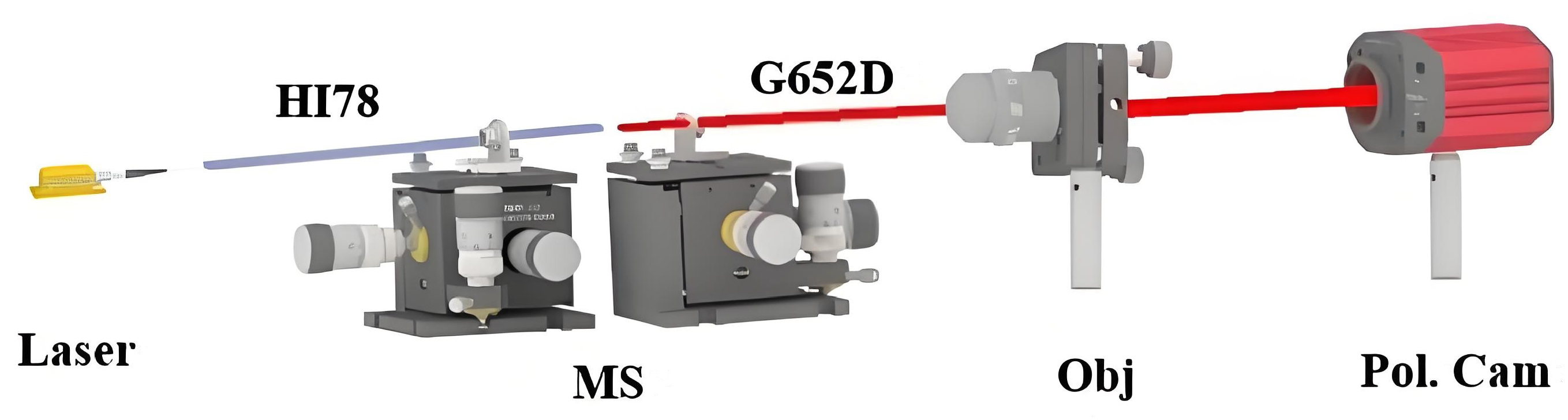
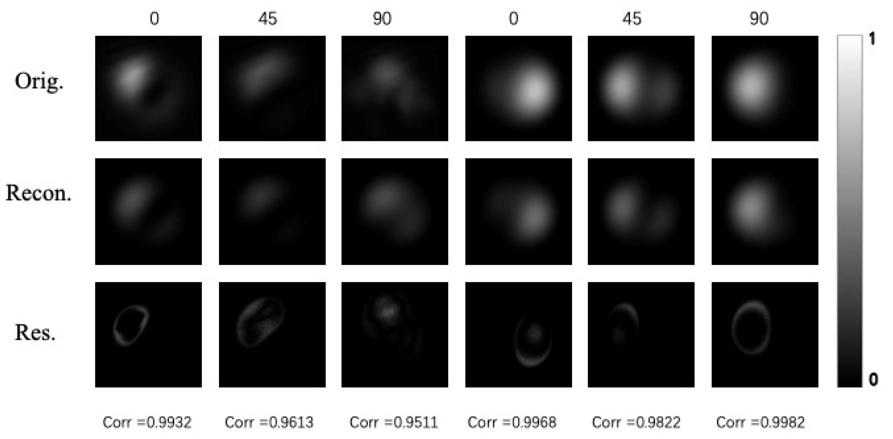
Next, we conducted a simulation to study the impact of noise on the algorithm’s performance. We added additive Gaussian white noise to the generated dataset using the following equation:

$$I_{noise k,j}^{\alpha }=max[0,I^{\alpha }+N(0,f)·max(I^{\alpha }\left)\right]$$

(15)

$N(0,f)$ is a random matrix with a normal distribution of the same size as $I^{\alpha }$. f is the noise factor, which determines the variance of the noise. The max function is used to prevent the occurrence of negative intensities.

The definition of SNR (signal-to-noise ratio) is as follows:

$$SNR\left(dB\right)=10lg\left[{\displaystyle \frac{{\sum }_{k=1}^{k=p}{\sum }_{j=1}^{j=p}{\left(I^{\alpha }\right)}^2}{{\sum }_{k=1}^{k=M}{\sum }_{j=1}^{j=M}{\left(I_{k,j}^{\alpha }-I_{noise k,j}^{\alpha }\right)}^2}}\right]$$

(16)

Figure 3 shows the impact of different block pixels L on the block mode decomposition error under the same signal-to-noise ratio and number of blocks B. The modal weights errors $e_{A_x}$ and $e_{A_y}$ decrease significantly as the block pixels L increase. When $L=1$, it corresponds to the sub-sample sampling method proposed in Ref. [23]. When L increases from 1 to 400, the errors drop rapidly. After L reaches around 1600, the errors stabilize and remain at a level of approximately ${10}^{-4}$. The phase errors also show a rapid decreasing trend when L increases from 1 to 400, but the reduction is not as pronounced as it is for amplitude errors. The phase errors level out around ${10}^{-3}$ at L = 4900, suggesting that further increases in L do not significantly improve decomposition accuracy.

Overall, Figure 3 indicates that amplitude errors decrease significantly with an increase in the number of block pixels. Although phase errors also decrease with an increase in block pixels, the reduction is less pronounced. Increasing L helps improve the accuracy of mode decomposition, particularly for amplitude errors.

Figure 4 illustrates the behavior of mode decomposition errors as a function of the number of blocks B. For SNR = 55 dB and $L=4900$, all the errors decrease as the number of blocks B increases. Notably, the amplitude errors exhibit the most pronounced decrease, with the errors rapidly decreasing from approximately ${10}^{-1}$ to below ${10}^{-4}$. At the same time, phase errors show a less dramatic decrease with an increase in B. After an initial decrease, these errors are around ${10}^{-2}$. The results indicate that increasing B significantly improves the accuracy of mode decomposition.

The computational load increases with the block size L and the number of blocks B, as the algorithm requires more multiplications and memory accesses. Larger blocks increase accuracy by capturing more local information but at the cost of processing time. However, as the B or L increases, the additional pixels in each block have a smaller impact on improving the accuracy, as the most significant contributions to phase error reduction have already been achieved with smaller block sizes. There may also be limitations related to the numerical resolution of the algorithm. Once the block size exceeds a certain threshold, the algorithm may reach its inherent resolution limit, beyond which further increases in block size offer little improvement. An optimal balance can be found depending on the specific application and computational constraints. In practice, it may be necessary to tune the block size and number of blocks to achieve an acceptable trade-off between accuracy and computational efficiency, depending on the available computational resources and the desired level of precision.

Different input image sizes also affect the mode decomposition algorithm’s performance: the MD error for M = 512 is generally lower than that for M = 128. For example, when B = 50, $e_{A_x}$ is $3\times {10}^{-5}$ for M = 512, while $e_{A_x}$ is $7\times {10}^{-4}$ for M = 128. For phase error, $e_{{\theta }_x}$ is $2\times {10}^{-3}$ for M = 512, while, for M = 128, $e_{{\theta }_x}$ is $3\times {10}^{-2}$.This suggests that larger input image sizes can provide more information, thereby improving decomposition accuracy and reducing error.

Figure 5 shows the mode decomposition error as a function of SNR, with different configurations of B. Panel (a) shows the amplitude error of the mode decomposition algorithms under varying SNR values. This panel highlights how the BMD algorithm performs with different block sizes (denoted as B) in comparison with the SPMD algorithm. Panel (b) shows the phase error of the mode decomposition algorithms under the same SNR conditions. All kinds of errors decrease as the SNR increases, which is expected since a higher SNR typically leads to better image quality and more accurate mode decomposition. The curves for larger B values (i.e., B = 30 or 50) show consistently lower errors compared to smaller B values (i.e., B = 10). For SNR = 70 dB, when B = 50, $e_{A_y}$ is $6\times {10}^{-6}$, and, when B = 10, $e_{A_y}$ is $2\times {10}^{-3}$. At the same time, for SNR = 70 dB, when B = 50, $e_{{\theta }_y}$ is $3\times {10}^{-3}$, and, when B = 10, $e_{{\theta }_y}$ is $5\times {10}^{-2}$. This indicates that increasing the number of selected blocks improves the decomposition accuracy across all SNR levels.

When the SNR is above 50 dB, both the amplitude and phase errors for both $B=30$ and $B=50$ are lower than those for the SPMD of $M=128$. For amplitude error, this algorithm outperforms 15 dB better than the SPMD at the error value of $3\times {10}^{-4}$, while, for phase error, it can outperform by 30 dB at error value of $3\times {10}^{-2}$, indicating that the BMD is better than SPMD.

3.2. Experiment

The performance of the block mode decomposition was further evaluated by employing actual near-field beam profile images, captured by a polarization camera. The detailed experimental setup for acquiring these real beam profile images is illustrated in Figure 6.

The laser emits light at a wavelength of 790 nm. By adjusting the knobs on the fiber linear motion stages, the relative position between the HI780 fiber and the single-mode fiber (a FullBand Low Water Peak Single-mode fiber from Yangtze Optical Fiber, Wuhan, China) can be varied, allowing for the excitation of different mode groups. The five-axis motion stages provide precise, smooth, and continuous adjustments, ensuring long-term stability. A $60\times$ magnification objective lens is used to enlarge the image, and a polarization camera (LUCID TRIO5051-PC from Lucid Vision in Richmond, British Columbia, Canada) captures images at four different polarization angles. A correlation metric is introduced for the comparative analysis between the captured image and the reconstructed image.

$$Corr=\left|{\displaystyle \frac{\int \int \Delta I_r(x,y)\Delta I_o(x,y)dxdy}{\sqrt{\int \int \Delta I_r^2(x,y)dxdy\int \int \Delta I_o^2(x,y)dxdy}}}\right|$$

(17)

Here, $\Delta I_{r\left(o\right)}=I_{r\left(o\right)}-\overline{I_{r\left(o\right)}}$, $I_r$, and $I_o$ represent the reconstructed and original field distributions, and $I_{r\left(o\right)}$ is the mean value of $I_r\left(o\right)$.

The captured images of pixel size $500\times 500$ are processed using BMD to calculate mode coefficients, which are then employed to reconstruct the field intensity distribution. A typical example of mode decomposition results is presented in Figure 7. This algorithm utilizes the field intensity distributions at polarization angles of $0^{\circ }$, ${45}^{\circ }$, and ${90}^{\circ }$ to recover the coefficients. As shown in Figure 7, when the number of modes is six, the correlation coefficients between the reconstructed images and the original images are all above 95%, indicating that this algorithm has practical applicability.

The correlation coefficient (Corr) is used as the evaluation metric to compare the original and reconstructed images. The recovery is also performed using the SPMD, and the results of the two algorithms are shown in

Table 1. Experimental results of SPMD and BMD (correlation).

	$0^{\circ }$	${45}^{\circ }$	${90}^{\circ }$
SPMD ($M=250$)	0.9855	0.9609	0.9200
BMD $B=50$ $L=4900$	0.9932	0.9613	0.9511

. It is worth noting that using SPMD requires 750,000 multiplication operations, while BMD only requires 30,000 multiplication operations. As can be observed from Table 1, the proposed algorithm exhibits better performance.

4. Conclusions

We propose a mode decomposition algorithm with sample blocks that, compared to our previously introduced SPMD algorithm, significantly reduces computational complexity while maintaining a high accuracy. We also analyze the algorithm’s performance under various SNR values, demonstrating that this algorithm offers better noise sustainability in noisy environments. When the SNR is greater than 40 dB, it achieves higher accuracy compared to the SPMD, which offers a new approach to improving the accuracy of mode decomposition.

References

1. Lv, J.; Li, H.; Zhang, Y.; Tao, R.; Dong, Z.; Gu, C.; Yao, P.; Zhu, Y.; Chen, W.; Zhan, Q.; et al. Few-mode random fiber laser with a switchable oscillating spatial mode. Opt. Express 2020, 28, 38973–38982. [Google Scholar] [CrossRef] [PubMed]
2. Chen, X.; Yao, T.; Huang, L.; An, Y.; Wu, H.; Pan, Z.; Zhou, P. Functional fibers and functional fiber-based components for high-power lasers. Adv. Fiber Mater. 2023, 5, 59–106. [Google Scholar] [CrossRef]
3. Zhang, X.; Gao, S.; Wang, Y.; Ding, W.; Wang, P. Design of large mode area all-solid anti-resonant fiber for high-power lasers. High Power Laser Sci. Eng. 2021, 9, e23. [Google Scholar] [CrossRef]
4. Wang, Y.; Tang, Y.; Yan, S.; Xu, J. High-power mode-locked 2 µm multimode fiber laser. Laser Phys. Lett. 2018, 15, 085101. [Google Scholar] [CrossRef]
5. Richardson, D.J.; Fini, J.M.; Nelson, L.E. Space-division multiplexing in optical fibres. Nat. Photonics 2013, 7, 354–362. [Google Scholar] [CrossRef]
6. Rademacher, G.; Puttnam, B.J.; Luis, R.S.; Eriksson, T.A.; Fontaine, N.K.; Mazur, M.; Chen, H.; Ryf, R.; Neilson, D.T.; Sillard, P.; et al. Ultra-wide band transmission in few-mode fibers. In Proceedings of the 2021 European Conference on Optical Communication (ECOC), Bordeaux, France, 13–16 September 2021; IEEE: Piscataway, NY, USA, 2021; pp. 1–4. [Google Scholar]
7. Zuo, M.; Ge, D.; Liu, J.; Gao, Y.; Shen, L.; Lan, X.; Chen, Z.; He, Y.; Li, J. Long-haul intermodal-MIMO-free MDM transmission based on a weakly coupled multiple-ring-core few-mode fiber. Opt. Express 2022, 30, 5868–5878. [Google Scholar] [CrossRef]
8. Qiu, Y.; Xu, J.; Wong, K.K.; Tsia, K.K. Exploiting few mode-fibers for optical time-stretch confocal microscopy in the short near-infrared window. Opt. Express 2012, 20, 24115–24123. [Google Scholar] [CrossRef]
9. Diab, M.; Dinkelaker, A.N.; Davenport, J.; Madhav, K.; Roth, M.M. Starlight coupling through atmospheric turbulence into few-mode fibres and photonic lanterns in the presence of partial adaptive optics correction. Mon. Not. R. Astron. Soc. 2021, 501, 1557–1567. [Google Scholar] [CrossRef]
10. Renninger, W.H.; Wise, F.W. Optical solitons in graded-index multimode fibres. Nat. Commun. 2013, 4, 1719. [Google Scholar] [CrossRef] [PubMed]
11. Wright, L.G.; Christodoulides, D.N.; Wise, F.W. Controllable spatiotemporal nonlinear effects in multimode fibres. Nat. Photonics 2015, 9, 306–310. [Google Scholar] [CrossRef]
12. Mangini, F.; Gervaziev, M.; Ferraro, M.; Kharenko, D.; Zitelli, M.; Sun, Y.; Couderc, V.; Podivilov, E.; Babin, S.; Wabnitz, S. Statistical mechanics of beam self-cleaning in GRIN multimode optical fibers. Opt. Express 2022, 30, 10850–10865. [Google Scholar] [CrossRef] [PubMed]
13. Shapira, O.; Abouraddy, A.F.; Joannopoulos, J.D.; Fink, Y. Complete modal decomposition for optical waveguides. Phys. Rev. Lett. 2005, 94, 143902. [Google Scholar] [CrossRef] [PubMed]
14. Brüning, R.; Gelszinnis, P.; Schulze, C.; Flamm, D.; Duparré, M. Comparative analysis of numerical methods for the mode analysis of laser beams. Appl. Opt. 2013, 52, 7769–7777. [Google Scholar] [CrossRef]
15. Lü, H.; Zhou, P.; Wang, X.; Jiang, Z. Fast and accurate modal decomposition of multimode fiber based on stochastic parallel gradient descent algorithm. Appl. Opt. 2013, 52, 2905–2908. [Google Scholar] [CrossRef]
16. Chen, F.; Zhao, S.; Wang, Q.; Ma, J.; Lu, Q.; Wan, J.; Xie, R.; Zhu, R. Modal decomposition of a fibre laser beam based on the push-broom stochastic parallel gradient descent algorithm. Opt. Commun. 2021, 481, 126538. [Google Scholar] [CrossRef]
17. Jiang, M.; Wu, H.; An, Y.; Hou, T.; Chang, Q.; Huang, L.; Li, J.; Su, R.; Zhou, P. Fiber laser development enabled by machine learning: Review and prospect. PhotoniX 2022, 3, 16. [Google Scholar] [CrossRef]
18. Tian, Z.; Pei, L.; Wang, J.; Hu, K.; Xu, W.; Zheng, J.; Li, J.; Ning, T. High-performance mode decomposition using physics-and data-driven deep learning. Opt. Express 2022, 30, 39932–39945. [Google Scholar] [CrossRef] [PubMed]
19. Yan, B.; Zhang, J.; Wang, M.; Jiang, Y.; Mi, S. Degenerated mode decomposition with convolutional neural network for few-mode fibers. Opt. Laser Technol. 2022, 154, 108287. [Google Scholar] [CrossRef]
20. Zhao, J.; Chen, G.; Bi, X.; Cai, W.; Yue, L.; Tang, M. Fast mode decomposition for few-mode fiber based on lightweight neural network. Chin. Opt. Lett. 2024, 22, 020604. [Google Scholar] [CrossRef]
21. Manuylovich, E.S.; Dvoyrin, V.V.; Turitsyn, S.K. Fast mode decomposition in few-mode fibers. Nat. Commun. 2020, 11, 5507. [Google Scholar] [CrossRef]
22. Wang, C.; Zhang, J.; Yan, B.; Mi, S.; Fan, G.; Wang, M.; Zhang, P. Spatially degenerated mode decomposition for few-mode fibers. Opt. Fiber Technol. 2024, 85, 103781. [Google Scholar] [CrossRef]
23. Choi, K.; Jun, C. Sub-sampled modal decomposition in few-mode fibers. Opt. Express 2021, 29, 32670–32681. [Google Scholar] [CrossRef] [PubMed]
Figure 1. Example of selection of blocks.
Photonics 12 00066 g001
Figure 2. Decomposition errors of noiseless images. (a) Amplitude errors; (b) phase errors.
Photonics 12 00066 g002
Figure 3. Mode decomposition error versus the number of block pixels L for SNR = 55 dB, N = 6 , and B = 50 .
Photonics 12 00066 g003
Figure 4. Mode decomposition errors versus the number of blocks B with the input pixel size M = 128 or 512, SNR = 55 dB, N = 6 , and L = 4900 .
Photonics 12 00066 g004
Figure 5. Mode decomposition errors and the signal-to-noise ratio (SNR) for N = 6 , L = 4900 , and M = 512.
Photonics 12 00066 g005
Figure 6. Experimental setup. MS: optic fiber linear motion stages, Obj.: objective lens, Pol. Cam: polarization camera.
Photonics 12 00066 g006
Figure 7. Results of block-based mode decomposition experiments when B = 50 L = 4900 , with the color bar indicating intensity (scaled from 0 to 1).
Photonics 12 00066 g007