Article

Modeling Femtosecond Beam Propagation in Dielectric Hollow-Core Waveguides

National Institute for R&D of Isotopic and Molecular Technologies, 400293 Cluj-Napoca, Romania
*
Author to whom correspondence should be addressed.
Photonics 2025, 12(1), 65; https://doi.org/10.3390/photonics12010065
Submission received: 18 December 2024 / Revised: 30 December 2024 / Accepted: 2 January 2025 / Published: 13 January 2025
(This article belongs to the Special Issue Advances in Ultrafast Laser Science and Applications)

Abstract

:
The propagation of femtosecond pulses in guided structures is a matter of both fundamental and practical interest in nonlinear optics. In particular, hollow-core waveguides (HCWs) filled with a gas medium are fabricated and used as devices for the generation of attosecond pulses from high-order harmonics. In this process, the configuration of the laser field (intensity and phase) inside the waveguide is of crucial importance for enhancing the (well-known, low) efficiency of high-order harmonic generation (HHG). Here, we present numerical calculations which demonstrate the main features of the propagation process in fabricated HCWs. We consider a variety of experimental parameters like gas pressure, waveguide size, laser wavelength, and pulse energy and duration. In particular, the beam profile at the fiber input is found to be a sensitive parameter which influences the whole evolution of the laser field along the propagation. Our model is based on a split-step method modified to account for propagation in ionized media and is validated against experimental and theoretical data from the literature. Our results contribute to the description of the main features of beam propagation in HCWs and provide guiding directions for designing efficient configurations for HHG.

1. Introduction

High-order harmonic generation (HHG) in gas media proves to be a valuable method to obtain extreme ultraviolet or soft X-ray attosecond pulses [1] and has received recognition from the scientific community, being the topic of the Nobel prize in physics awarded in 2023 [2]. The basic elementary process is simple and intuitively easy to understand via the three-step [3] model: the interaction between the atom and the intense electric field of the laser pulse which produces the ionization of an outer shell electron, its acceleration outside the atom, and finally its recombination with the parent atom which generates a burst of light for a single attosecond. The gas medium is usually supplied in a jet or in a static cell [4], but the alternative of using structures to host the gas and to guide the ultrafast beam over longer distances is currently being investigated to increase HHG efficiency. Such structures, in particular dielectric hollow-core waveguides [5,6] custom-fabricated in various configurations, demonstrate that they are capable of keeping both the gas at high pressures and a high laser intensity over longer interaction lengths.
Solving the field configuration inside an HCW is of basic importance for optimizing HHG. The main way to increase HHG yield is to create conditions for phase matching, that is, to have constructive interference between single atomic emissions and the harmonic field built up in a specific point. One can estimate the phase-matching conditions by finding the phase of the driving field in the interaction region, as well as the phase of the atomic polarization which is proportional to the driving field intensity. Solving the propagation problem in an HCW, that is, finding the intensity and phase of the driving field, is therefore a first step in estimating the efficiency of HHG. Second, solving the propagation equation helps experimentalists to find the appropriate configurations for the waveguide and for the focusing conditions such as obtaining and keeping a high field intensity along the HCW, which is an important factor to contribute to the HHG yield and cutoff.
There is active research trying to uncover the advantages of using gas-filled HCWs and to explore the regimes of pulse propagation in guided conditions. For example, a recent study [7] demonstrates that a plasma-induced flat-top beam can be formed in these structures, similarly to free space propagation [8]. An attractive field considers the use of mid-infrared wavelengths like 1.3 μm [9] or 3.9 μm and multi-athmosphere pressures [10] to generate attosecond pulses in the soft X-ray and water window region.
The propagation of femtosecond pulses in HCWs is used as a method to shorten the femtosecond pulse duration first by inducing a spectral broadening of the pulse [11] and then by applying various post-compression techniques to the propagated pulse. In this way, one obtains few cycle pulses, especially in the mid-IR range [12] and for high-energy pulses [13,14]. For these cases, solving the wave equation for configurations similar to experimental conditions generates data about the spectral/temporal characteristics of the propagated pulse and helps design the parameters of broadening and post-compression in advance.
In this paper, we present laser field characteristics inside an HCW as a function of a number of pulse/beam parameters, which are of significant importance in HHG experiments. The structure of the paper is as follows: in Section 2, we present the numerical framework and methods to solve the propagation equation. This section also includes results on testing the validity of the method and on mode beating along the propagation direction. Section 3 contains results showing the spatial configuration of the laser field in a standard cylindrical HCW and in modulated waveguides. Finally we present results which demonstrate that some parameters of pulse propagation and harmonic generation in HCWs can be invariantly scaled and identify the specific scaling relations for these parameters.

2. Model and Methods

The pulsed field propagation in an HCW is solved by starting from the wave equation in time domain,
2 E 1 ( r , z , t ) 1 c 2 2 E 1 ( r , z , t ) t 2 = ω 2 c 2 ( 1 η e f f 2 ) E 1 ( r , z , t )
Here, ω is the central angular frequency of the driving field, while η e f f is the space- and time-dependent effective refractive index of the medium:
η e f f ( n a , n e , r , z , t ) = η 0 ( n a ) + η 2 ( n 0 ) I ( r , z , t ) ω p 2 ( n e , r , z , t ) 2 ω 2
According to Equation (2), the refractive index includes three contributions: The first term accounts for the linear dispersion and absorption and depends on the density of the neutral atoms n a . The second term contains the intensity-dependent nonlinear refractive index which represents the optical Kerr effect. Here, n 0 is the total particle density and I ( r , z , t ) is the instantaneous laser intensity. The last term accounts for plasma defocusing, where ω p is the plasma angular frequency and n e is the free electron density. Since ionization is the first step during laser–atom interaction, the plasma formation is inevitable in the interaction volume. In most cases, this last term dominates the fast variation in the medium’s refractive index.
The next step is transforming Equation (1) in a frame ( r , z ) moving with the speed of light c and then in the frequency domain by applying a Fourier transform, F ^ , and, after making use of the paraxial approximation, it becomes
2 E 1 ˜ ( r , z , ω ) 2 i ω c E 1 ˜ ( r , z , ω ) z = G ˜ ( r , z , ω )
where
E 1 ˜ ( r , z , ω ) = F ^ E 1 ( r , z , t )
is the Fourier transform of E 1 ( r , z , t ) , and
G ˜ ( r , z , ω ) = F ^ { ω p 2 c 2 E 1 ( r , z , t ) 2 ω 0 2 c 2 δ 1 + η 2 I ( r , z , t ) E 1 ( r , z , t ) }
is the Fourier transform of the free term.
This model, with appropriate boundary conditions, has been used for propagation in free space [15], but here it was adapted for propagation in a guided structure by using the split-step method [16]. In the first step, we solved the homogeneous version of Equation (3) which contains only the diffraction term on the left-hand side and a null term on the right hand side. The boundary conditions inside the HCW were imposed by writing the solution as the superposition of the hybrid EH 1 m eigenmodes [17]:
E 1 ˜ ( r , z , ω ) = j b j ( z , ω ) J 0 ( u 1 j r / a ) exp i 0 z γ j ( z ) d z
where u 1 j are the roots of the Bessel function of the first kind J 0 , a is the inner radius of the fiber, and γ j ( z ) is the propagation constant as defined in [17], while
b j ( z = 0 ) = 2 a 2 J 1 2 ( u i j ) 0 a r J 0 ( u 1 j r a ) E 1 ( r ) d r
are the coefficients in the expansion.
In the first step, we advanced one d z step in the homogeneous part of Equation (3), and this could be performed by writing E 1 ( z + d z ) using Equation (5) and taking into account the orthonormality properties of the b j coefficients. With the new coefficients b j ( z + d z , ω ) , we rebuilt the field E 1 ( z + d z ) and proceeded to the second step, in which we solved the ordinary differential equation
2 i ω c E 1 ˜ ( r , z , ω ) z = G ˜ ( r , z , ω )
which is in fact Equation (3) without the diffraction term. At this point, we must observe that the free term in Equation (7) is dependent on the solution itself, and for this reason, we applied an iterative procedure to solve this equation. First, (i) we Fourier transformed the field E 1 ( r , z , ω ) to obtain E 1 ( r , z , t ) ; then, (ii) we recalculated the free term G ( r , z , t ) in the time domain and used Equation (4) to obtain G ˜ ( r , z , ω ) . Finally, (iii) we solved the first-order differential equation over the same d z step and obtained a new E 1 ( r , z , ω ) . The steps from (i) to (iii) were repeated until the difference between two successive solutions was below a specified threshold. Depending on the level of gas ionization, gas pressure, gas nature, etc., three to ten iterations were necessary to reach convergence.

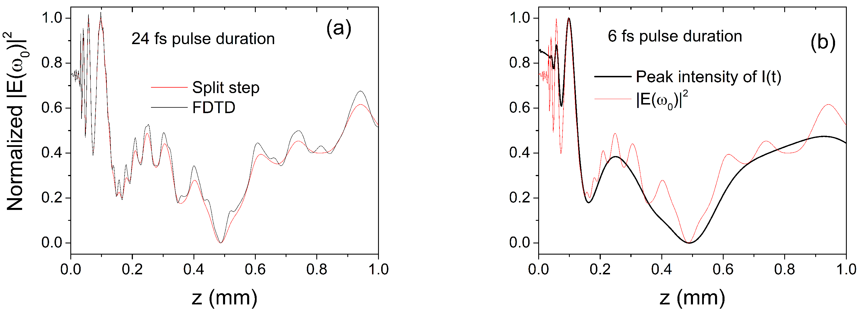
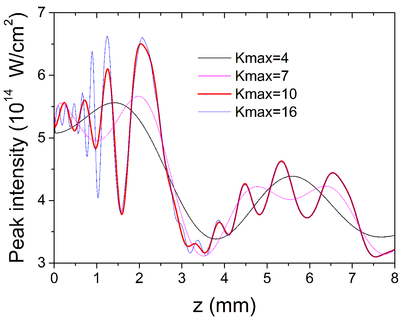
Testing and Tuning the Split-Step Method

Testing the split-step method against experimental data was a necessary step in the model’s development. The simulation results of the model for conditions close to a specific experimental situation [18] have been reported earlier [19]. Here, we just mention that a very good agreement was found between the dependence along the propagation direction of Ar fluorescence and the total electron density obtained from simulations. Successful tests were also performed against results [20] obtained from solving the Schrodinger equation for pulse propagation in the HCW.
Testing against other accepted numerical methods for solving the propagation equation was also a necessary step. The result of a finite-difference time-dependent (FDTD) calculation using Lumerical software [21] is shown in Figure 1a together with our split-step calculation performed for an HCW with a radius of a = 15 microns. Both calculations were performed in three-dimensional geometry for a pulse of 24 fs focused at the HCW’s entrance with the best coupling condition of a waist of w = 0.64 · a . In Figure 1a, the spectral component corresponding to the central frequency is shown for both calculations. We also performed a similar calculation for a 6 fs pulse. While the spectral components were in agreement for both calculations, the peak intensity of I ( t ) calculated with the split-step method is different, having a more smooth dependence on the propagation distance. The larger spectral width of the 6 fs pulse also means that there were more spectral amplitudes with different variations along the propagation direction and, as a result, the Fourier transform of the spectral field had a smoother dependence along the HCW axis. This can be important for the HHG process as the dipole phase is proportional to the field intensity, so shorter pulses may give better phase-matching conditions.
As one can note from Figure 1a, there are small differences in the field amplitude but the overall agreement is good; the field variations are the same in both cases. Here, we mention that we also used an eigenmode expansion method also implemented in Lumerical [21], and a good agreement was also obtained. This method was closer to the split-step method as it made use of the electromagnetic field’s decomposition into a basic set of local eigenmodes that existed in the cross section of the HCW.
In building the propagated field from the normal modes (Equation (5)), we studied how many modes ensured the convergence of the field. Given in Figure 2 are the results obtained in various runs using an increasing number of modes, specified as K m a x . Here, we note that K m a x < 10 did not produce convergent results, but after a sufficiently long propagation distance, the runs with K m a x = 10 and K m a x = 16 yielded almost coincident fields. However, more modes are necessary when the propagation distance is less than 1000 times the central wavelength of the driving field or in higher-ionization conditions [22].
A dominant feature of pulse propagation in a multimode HCW is the beating of the normal modes of the fiber [23,24]. We investigated how this mode beating influences the field configuration both in a vacuum and in gas in a number of configurations, both for cylindrical and for conical waveguides. The beating spatial period is proportional to a 2 / λ , with a being the guide radius and λ the central wavelength; thus, for a conical HCW, the periodicity of the intensity variation decreases as the radius a decreases. As we will see further, this conical configuration prevents the decrease in the intensity, and this has importance in HHG.
It is interesting to see how the normal modes participate in building up the total field. In Figure 3, we show the energies of the first ten modes for both Gaussian (Figure 3a) and Bessel (Figure 3b) initial radial profiles (IRPs) for different propagation distances, specified in the legends. The Gaussian profile was injected with less than 1 mJ of energy because, even at optimal coupling, the beam was truncated, so the peripheral energy was lost. After 8 mm of propagation, higher-order modes, EH 1 m , with 2 < m < 10 contained energies from 2 μJ down to 0.01 μJ and the mode energy showed a slower decrease with an increasing order.
For the Bessel IRP, we see in Figure 3b that the fundamental mode had 1 mJ of energy (which was the total pulse energy injected in the HCW) while all normal modes with an index of m > 1 contained practically negligible energies ( E < 10 11 mJ). Advancing the propagation, we noted an increase in their energies so that after 8 mm the modes EH 12 and EH 13 had 1% and 0.1%, respectively, of the EH 11 energy, with higher-order modes having down to 10 8 mJ. From these data, one can estimate the number of normal modes necessary for an accurate description of the propagated field. In our cases, for the Gaussian IRP, we used between 15 and 20 normal modes.
Other radial profiles at the HCW’s input can be considered, such as Airy or super-Gaussian profiles, depending on the experimental setup. However, the most common and frequent, the Gaussian profile, must be investigated in order to have the modeling as close as possible to the experiment. Imperfect coupling like a non-optimal beam size, oblique incidence, and focus position with respect to the input plane are currently under our investigation.

3. Results and Discussion

The input parameters of the model were usually selected to be closely connected to the experimentally measurable values: the pulse energy and duration, central wavelength, focusing geometry, gas pressure, and HCW size. The model allowed for a variety of beam profiles in the injection plane (Gaussian, truncated Gaussian, Bessel, etc.) as well as for an arbitrary pressure profile along the z direction. The initial field could be specified in the time or frequency domain.
The main result of the model was the electric field, E 1 ( r , z , t ) , or equivalently E 1 ( r , z , ω ) , inside the HCW, but additional results included ( r , z ) maps of the peak intensity and phase of the electric field, as well as maps of the electron density and refractive index result after propagation. Other quantities like the pulse energy, mode energies, mode amplitudes, and spectral characteristics of the field could be extracted from the calculation.

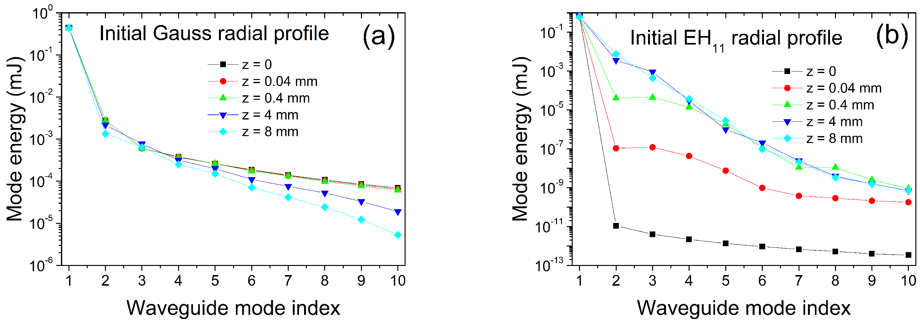
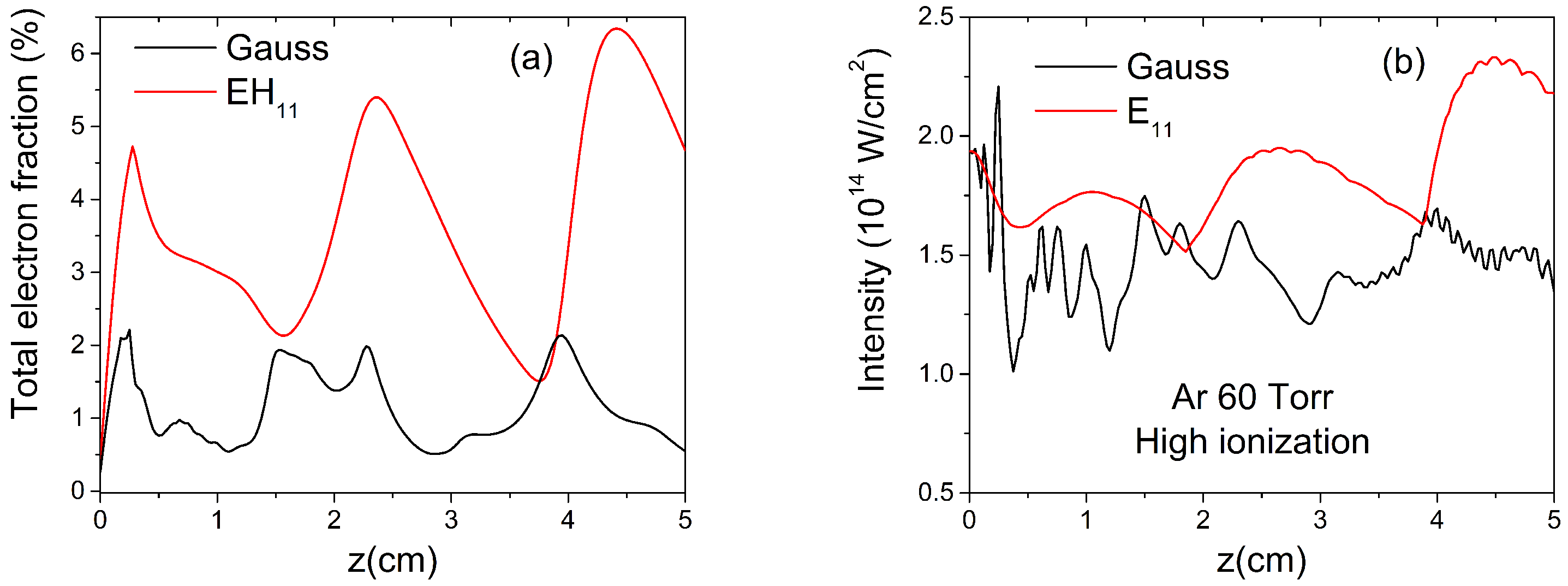
3.1. Influence of Initial Beam Profile in Injection Plane

For technical reasons, many of the calculations reported in the literature [25,26] assume that the IRP of the field at the entrance of an HCW is a Bessel profile. Indeed, the Gaussian with a waist at an optimal coupling value, w = 2 a / π , is very close to the fundamental mode E 11 of propagation, which is a Bessel J 0 ( r / a ) profile. As one can check in a simple calculation, in HCW walls, the difference between the intensities of the two profiles is less than 1%. However, we found that the propagation along the HCW was noticeably dependent on the choice of the IRP. Figure 4 demonstrates this by showing the on-axis peak intensity for the two profiles at two different He pressures, 50 and 500 torr, in an 8 mm-long HCW, with a radius of 70 μm. The difference comes from the modal decomposition (Equation (5)) of the two profiles. While the Bessel profile contained mainly the fundamental mode, the Gauss profile also needed higher-order modes to be described properly, and during propagation, the beating of these modes produced the oscillations of the total field.
The effect of pressure for the two profiles is also shown in Figure 4. Here, the initial ionization is low (around 1%), so the mode beating dominates the field behavior, and the pressure value or pressure distribution has only a secondary role in shaping the field map. The fact that the mode beating is dominant over the pressure value or pressure distribution has significance for HHG experimentalists as it gives a higher degree of freedom in choosing the pressure which is favorable for phase matching.
For a gas with a lower ionization potential (Ar, 60 torr, 11% peak electron fraction), we show the radially integrated electron fraction in Figure 5a and the on-axis peak intensity in Figure 5b. Here, ionization plays an increasing role, and the Bessel profile also starts showing mode beating. Indeed, plasma defocusing alters the initial EH 11 profile and higher modes come into play in order to describe the radial profile. However, the Gaussian case shows a much closer agreement with Ar fluorescence measurements [27], reproducing the position of the peaks and even the structure of the middle peak at z = 2 cm.
For the Gaussian IRP, we also investigated the influence of imperfect coupling on the field configuration. With reference to the optimal coupling in which the waist is w = 2 / π · a 0.64 · a , we plot in Figure 6 the on-axis field dependence on the propagation distance for two other cases: w = 0.61 · a (tighter focusing) and w = 0.67 · a (weaker focusing). The initial field intensity is different but one can see that the mode beating yields similar field oscillations; however, there is a higher/smaller contrast for weaker/tighter focusing. This kind of result is useful for experimental situations in which the input plane inside the HCW does not coincide with the focusing plane of the beam. The result presented in Figure 6 suggests that this lack of coincidence is not very critical.

3.2. Beam Propagation in Modulated HCW

In various principle methods for HCW fabrication, we can build a large variety of HCW geometries as well as various configurations for the gas flow inside the architecture of the setup. The combination of these parameters can lead to interesting results concerning the efficiency of the HHG process but also the spectral structure of the attosecond pulse trains. One of the structures we want to consider for an HHG experiment is the HCW with a variable diameter. In such a structure, the mode beating has a variable period so in principle one could control the evolution of the laser intensity and phase in order to optimize the HHG yield.
We take here the simple cases of one cylindrical and two conical HCWs, the first one with a constant diameter of 150 μm and the other two being conically convergent (divergent) and having a linearly variable diameter starting from 150 (110) μm at the beam input and ending after 8 mm with a diameter of 110 (150) μm. A pulse of a 25 fs duration, 0.6 mJ energy, and 800 nm central wavelength propagated in He gas at a 1100 torr peak pressure. The input peak intensity depended on the initial waveguide diameter as we imposed the best coupling in each case. The on-axis peak intensities along the waveguide are shown in Figure 7 for the three cases and demonstrate that by modulating the HCW diameter one could control the evolution of the intensity (and phase, not shown here) inside the HCW. For example, to prevent the decrease in the intensity in the second part of the waveguide, due to pulse energy losses, one could use the conically convergent waveguide. Using a similar configuration and a driving field of a wavelength centered at 2000 nm, we demonstrated that a harmonic field enhancement could be obtained in spectral domains of great practical interest, from 2.8 to 20 nm [28].
We also studied the case of micro-modulations in the HCW’s diameter, that is, the ripples which came out from the fabrication process. The calculations are reported elsewhere [19] and show that there were corresponding modulations in the field intensity, having the same periodicity; but, modulations have small amplitudes, so the overall evolution remained the same as for an ideal waveguide. In addition, the evolution of the pulse energy confirmed that the ripples enhanced the losses in the channel during propagation.

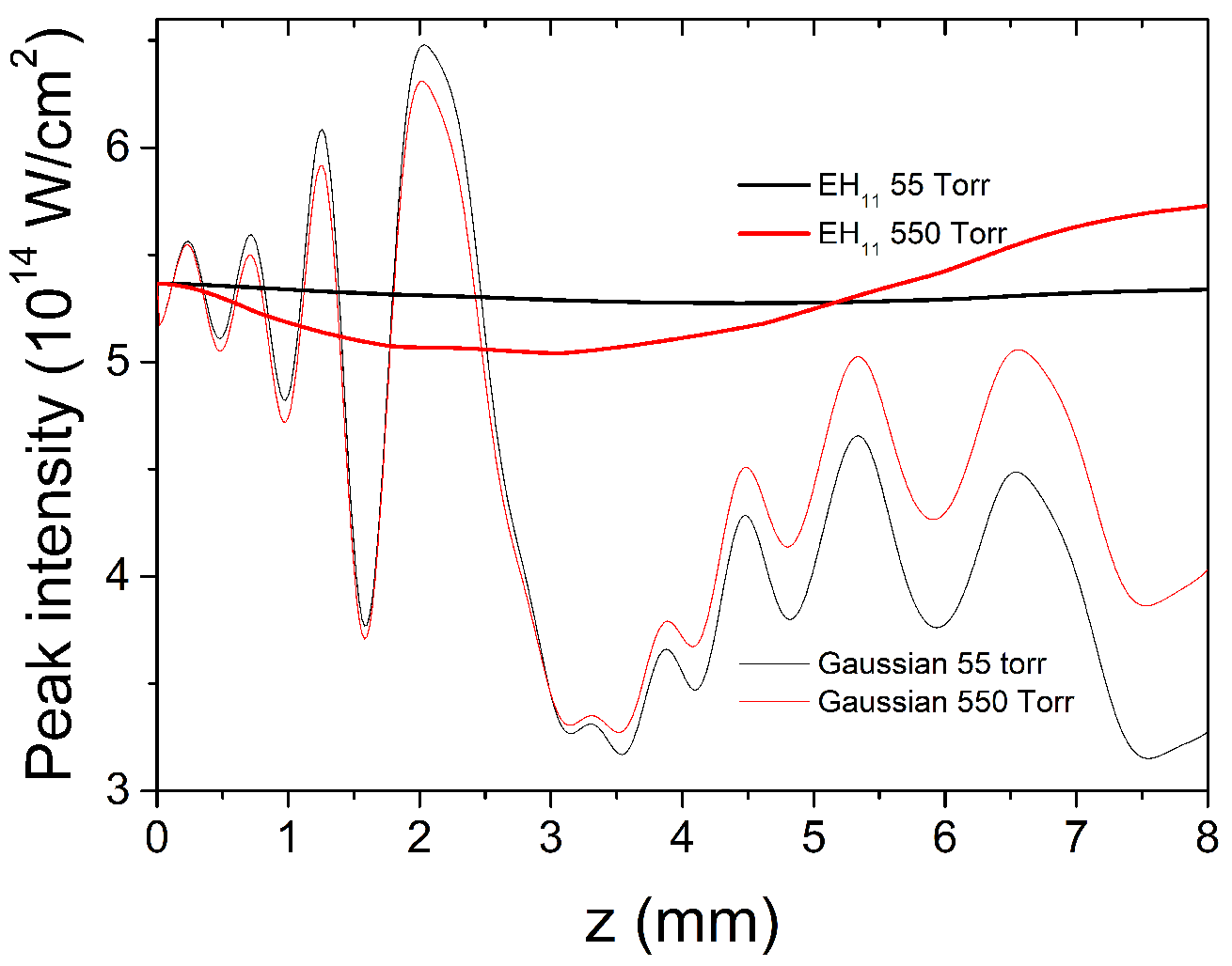
3.3. Scaling Femtosecond Pulse Propagation in HCW

As shown by Heyl et al. [29], paraxial nonlinear wave equations are scale-invariant if spatial dimensions, gas density, and laser pulse energy are scaled appropriately. This scaling applies also to the fields generated in nonlinear interactions like high-order harmonics; therefore, it is of practical importance to see if this scaling is also valid for HCW configurations. As demonstrated for the case of pulse propagation in free space [29], any spatial and temporal modifications of the field induced by diffraction, dispersion, or a nonlinear process are scale-invariant provided this nonlinear process is proportional to the medium density. A demonstration of this scaling was performed via modeling for the case of beam filamentation and harmonic generation in gas media, in which gas pressure (density) was also scaled as p p / f 2 .
The propagation Equation (3) for the electric field in the frequency domain is invariant under the transformations specified in [29]: r f r , z f 2 z , and E p u l s e f 2 E p u l s e , where f is the scaling factor, r and z are the spatial coordinates, and E p u l s e is the pulse energy (input or output). However, the solution of this equation is dependent on the boundary conditions which are imposed by the propagation in a guided medium. As we saw in previous sections, mode beating has a clear influence on propagation and induces field intensity oscillations along the axis of the guide. It is therefore of interest to identify the conditions in which the scaling applies for propagation in an HCW.
We analyzed two cases in which, essentially, the level of plasma density was different. Shown in Figure 8a is the on-axis field intensity for the propagation in He gas at a 300 torr maximum pressure and an electron fraction of about 3%. The basic case was a waveguide of a radius of a = 35 μm and length of L = 8 mm which propagated a pulse of 0.2 mJ of energy and a 35 fs duration. The scaled-down case with a factor of f = 2 yielded a length of L = 4 mm, a = 35/ 2 μm, a 600 torr maximum pressure, and a 0.1 mJ pulse energy. In both cases, the best coupling condition was imposed, with the waist in focus in the input plane being 2 / π · a . If we estimate the rms error, ( I b I s ) 2 / N , between the basic ( I b ) and the scaled ( I s ) sets of N values, we obtain 0.03, namely a very good scaling process.
In order to estimate the influence of mode beating on scaling, we also ran a case which was scaled down with f = 2 , but the pressure was kept at 300 torr, as was L = 8 mm. The agreement was worse, with the rms error being 0.054, so it was almost double, but all the details of the intensity variation along the propagation distance were preserved. This indicates that at a low plasma density (which usually has the main contribution in the refractive index but here was not dominant), the scaling was mainly due to the mode beating. Indeed, the period of the mode beating was proportional to a 2 / λ , so it obeyed the same scaling with the propagation distance. In passing, we should mention that the comparison between the split-step method used here and the Lumerical calculation was performed in conditions of scaling, and this is clearly seen when one compares Figure 1a to Figure 8a.
For the high-plasma-density case, all parameters were kept from the low-plasma case, but the pulse energy was 0.4 mJ for the basic configuration, which created around a 58% electron fraction. As one can note in Figure 8b, the dependence on the propagation direction was clearly different from the low-intensity case, especially in the second half of the HCW. Here, the rms error was 0.23 so worsened with respect to the low-intensity case, but the agreement was still good. Here again, we tested the influence of mode beating on scaling by running a scaled-down case in which we kept a 300 torr pressure. As seen in Figure 8b, the intensity along the axial direction preserved some of the features from the basic configuration but had shifts in the spatial dimension and value; the rms error was 1.13 so scaling was not valid anymore. In this case we can say that the mode beating preserved some features of the propagation, but when the pressure was not scaled properly, the electron plasma broke the scaling.
It is interesting to understand the reason for the different evolution in the intensity along the HCW in high-ionization conditions. The effective refractive index given by Equation (2) includes two positive contributions (dispersion and Kerr) and a negative one proportional to electron density. We illustrate this in Figure 9a, where we plot ( 1 η e f f ( r , z ) ) , where η e f f ( r , z ) is the effective refractive index (Equation (2)) generated by the pulse itself at 0.4 mJ of energy. Figure 9b shows the electron fraction map which has the same pattern as the effective refractive index and proves the strong dependence of the propagation conditions on electron plasma. Having in mind the radial decrease in the intensity, we see that in regions close to the HCW axis, the refractive index is less than 1 but increases towards unity in the peripheral parts close to the HCW walls. In this way, electron plasma creates an additional (self-) guiding structure [8] with a size smaller than that of the HCW radius which influences the periodicity of intensity oscillations. One can see from these two maps that the guiding structure with a refractive index less than the unity extends up to about 20 μm. To check this assumption, we ran a low-intensity propagation in an HCW of a 20 μm radius and obtained a succession of maxima and minima in roughly the same positions as the high-intensity case shown in Figure 8b.

3.4. Scaling High-Order Harmonic Generation

Once the driving field was calculated in a grid inside the waveguide, we calculated the single-atom polarization P n l ( r , z , t ) over the same grid and then integrated the wave equation for the harmonic field E h ( r , z , t ) . This equation is similar to Equation (1) for the driving field except for the free term which is the second derivative in time of P n l ( r , z , t ) and is the source for the harmonic field. The non-linear polarization was calculated by solving the Lewenstein integral using the strong-field approximation. Further, the obtained polarization is the source term for solving the wave equation which describes the propagation of the generated harmonics. A detailed description of this method can be found in [28].
The Fourier transform of the time-dependent harmonic field allowed us to see how individual harmonics were built up inside the waveguide. Given in Figure 10 are the maps of the harmonic of the order 85 for the basic (a) and scaled-down (b) configurations. As one can see, the build-up process is very similar for the two cases. The small difference which can be seen towards the exit of the HCW is linked to the small differences seen in Figure 8b between the basic and the scaled cases. One can also see in both maps that the harmonic field exhibits spatial fringes as a function of both radial and axial coordinates. We assume that this structure is probably due to the build-up process in conditions of a short coherence length.
The scaling law for the harmonic field is especially important for guided propagation. If we integrate the harmonic field over the radial direction, we obtain the power spectrum. In the case of scaling, the field remains constant but the power spectrum scales with f . While scaling in free space is limited by beam defocusing which induces a decrease in the driving intensity for the case of an HCW, this decrease is not so dramatic and the validity of the scaling is less limited. Here, we have to mention that the scaling conditions of high-order harmonics generated by two-color waveforms incident into a gas-filled hollow waveguide were analysed in detail in [25].

4. Conclusions

In conclusion, we investigated via numerical modeling the propagation of femtosecond pulses and high-order harmonics generated in dielectric hollow-core waveguides. The beam profile in the injection plane was found to be a critical choice for a realistic modeling. The imperfect coupling of the beam with the HCW was accounted for, and its importance for the experiment was estimated. Beam propagation in HCWs of variable sizes was identified as a feasible way to control the evolution of the pulse along the waveguide. Finally, the scaling of beam propagation and harmonic generation was investigated, and the role of ionization in combination with guiding was demonstrated.
We built this model having in mind the necessity of exploring HHG in fabricated HCWs which can be used in modulated geometries not explored until now. The recent result of the model foresees the possibility of generating photons with wavelengths down to the water window [28] by using conical waveguides. Here, we demonstrate that one can also control the field intensity inside an HCW for Ti:Sa lasers at 800 nm. Applying scaling for HHG in these kinds of new geometries opens a vast field of research aimed at obtaining a high flux in photons in spectral regions of a high level of practical interest.

Author Contributions

Conceptualization, methodology, software, V.T.; validation, A.M.M.G., K.K. and I.T.; investigation, V.T. and A.M.M.G.; writing—original draft preparation, V.T.; writing—review and editing, A.M.M.G., K.K. and I.T.; supervision, V.T. All authors have read and agreed to the published version of the manuscript.

Funding

This project received funding from the European Union’s Horizon 2020 Research and Innovation Programme under Grant Agreement No. 964588 (XPIC).

Data Availability Statement

The data that support the findings of this study are available from the corresponding author upon reasonable request.

Conflicts of Interest

The authors declare no conflicts of interest.

References

  1. Calegari, F.; Ferrari, F.; Lucchini, M.; Negro, M.; Vozzi, C.; Stagira, S.; Sansone, G.; Nisoli, M. Chapter 8—Principles and Applications of Attosecond Technology. In Advances in Atomic, Molecular, and Optical Physics; Arimondo, E., Berman, P., Lin, C., Eds.; Academic Press: Cambridge, MA, USA, 2011; Volume 60, pp. 371–413. [Google Scholar] [CrossRef]
  2. The Nobel Prize in Physics 2023. NobelPrize.org. Nobel Prize Outreach. Available online: https://www.nobelprize.org/prizes/physics/2023/summary/ (accessed on 28 February 2024).
  3. Corkum, P.B. Plasma perspective on strong field multiphoton ionization. Phys. Rev. Lett. 1993, 71, 1994–1997. [Google Scholar] [CrossRef] [PubMed]
  4. Midorikawa, K. Progress on table-top isolated attosecond light sources. Nat. Photonics 2022, 16, 267–278. [Google Scholar] [CrossRef]
  5. Horak, P.; Poletti, F. Multimode Nonlinear Fibre Optics: Theory and Applications. In Recent Progress in Optical Fiber Research; Yasin, M., Harun, S.W., Arof, H., Eds.; IntechOpen: Rijeka, Croatia, 2012; Chapter 1. [Google Scholar] [CrossRef]
  6. Ciriolo, A.G.; Martínez Vázquez, R.; Crippa, G.; Devetta, M.; Faccialà, D.; Barbato, P.; Frassetto, F.; Negro, M.; Bariselli, F.; Poletto, L.; et al. Microfluidic devices for quasi-phase-matching in high-order harmonic generation. APL Photonics 2022, 7, 110801. [Google Scholar] [CrossRef]
  7. Li, B.; Wang, K.; Tang, X.; Zhang, C.; Wang, B.; Jin, C. Elimination of chromatic aberration in high-order harmonic generation using a plasma-induced flat-top beam in a gas medium. Phys. Rev. A 2024, 110, 043511. [Google Scholar] [CrossRef]
  8. Major, B.; Kovács, K.; Tosa, V.; Rudawski, P.; L’Huillier, A.; Varjú, K. Effect of plasma-core-induced self-guiding on phase matching of high-order harmonic generation in gases. J. Opt. Soc. Am. B 2019, 36, 1594–1601. [Google Scholar] [CrossRef]
  9. Popmintchev, T.; Chen, M.C.; Bahabad, A.; Gerrity, M.; Sidorenko, P.; Cohen, O.; Christov, I.P.; Murnane, M.M.; Kapteyn, H.C. Phase matching of high harmonic generation in the soft and hard X-ray regions of the spectrum. Proc. Natl. Acad. Sci. USA 2009, 106, 10516–10521. [Google Scholar] [CrossRef]
  10. Popmintchev, T.; Chen, M.C.; Popmintchev, D.; Arpin, P.; Brown, S.; Ališauskas, S.; Andriukaitis, G.; Balčiunas, T.; Mücke, O.D.; Pugzlys, A.; et al. Bright Coherent Ultrahigh Harmonics in the keV X-ray Regime from Mid-Infrared Femtosecond Lasers. Science 2012, 336, 1287–1291. [Google Scholar] [CrossRef]
  11. Ran, Q.; Li, H.; Chang, W.; Wang, Q. Self-Compression of High Energy Ultrashort Laser Pulses. Laser & Photonics Reviews 2024, 18, 2300595. [Google Scholar] [CrossRef]
  12. Fan, G.; Balčiūnas, T.; Kanai, T.; Flöry, T.; Andriukaitis, G.; Schmidt, B.E.; Légaré, F.; Baltuška, A. Hollow-core-waveguide compression of multi-millijoule CEP-stable 3.2 μm pulses. Optica 2016, 3, 1308–1311. [Google Scholar] [CrossRef]
  13. Tamas Nagy, P.S.; Veisz, L. High-energy few-cycle pulses: Post-compression techniques. Adv. Phys. X 2021, 6, 1845795. [Google Scholar] [CrossRef]
  14. Nagar, G.C.; Shim, B. Study of wavelength-dependent pulse self-compression for high intensity pulse propagation in gas-filled capillaries. Opt. Express 2021, 29, 27416–27433. [Google Scholar] [CrossRef]
  15. Tosa, V.; Kovács, K.; Major, B.; Balogh, E.; Varjú, K. Propagation effects in highly ionised gas media. Quantum Electron. 2016, 46, 321. [Google Scholar] [CrossRef]
  16. Nurhuda, M.; Suda, A.; Midorikawa, K.; Hatayama, M.; Nagasaka, K. Propagation dynamics of femtosecond laser pulses in a hollow fiber filled with argon: Constant gas pressure versus differential gas pressure. J. Opt. Soc. Am. B 2003, 20, 2002–2011. [Google Scholar] [CrossRef]
  17. Marcatili, E.A.J.; Schmeltzer, R.A. Hollow metallic and dielectric waveguides for long distance optical transmission and lasers. Bell Syst. Tech. J. 1964, 43, 1783–1809. [Google Scholar] [CrossRef]
  18. Froud, C.A.; Chapman, R.T.; Rogers, E.T.F.; Praeger, M.; Mills, B.; Grant-Jacob, J.; Butcher, T.J.; Stebbings, S.L.; de Paula, A.M.; Frey, J.G.; et al. Spatially resolved Ar* and Ar+* imaging as a diagnostic for capillary-based high harmonic generation. J. Opt. A Pure Appl. Opt. 2009, 11, 054011. [Google Scholar] [CrossRef]
  19. Tosa, V.; Ciriolo, A.G.; Vazquez, R.M.; Vozzi, C.; Stagira, S. Modeling femtosecond pulse propagation and high harmonics generation in hollow core fibers. EPJ Web Conf. 2021, 255, 11005. [Google Scholar] [CrossRef]
  20. Poletti, F.; Horak, P. Description of ultrashort pulse propagation in multimode optical fibers. J. Opt. Soc. Am. B 2008, 25, 1645–1654. [Google Scholar] [CrossRef]
  21. Ansys Lumerical Inc. 2022. Available online: https://www.ansys.com/products/optics (accessed on 1 November 2024).
  22. Li, B.; Wang, K.; Tang, X.; Wang, B.; Lin, C.D.; Jin, C. Enhancement of harmonic generation by an intense driving laser with high-order waveguide modes in a high-pressure gas-filled hollow waveguide. Opt. Express 2024, 32, 48972–48986. [Google Scholar] [CrossRef]
  23. Dromey, B.; Zepf, M.; Landreman, M.; Hooker, S.M. Quasi-phasematching of harmonic generation via multimode beating in waveguides. Opt. Express 2007, 15, 7894–7900. [Google Scholar] [CrossRef]
  24. Zepf, M.; Dromey, B.; Landreman, M.; Foster, P.; Hooker, S.M. Bright Quasi-Phase-Matched Soft-X-Ray Harmonic Radiation from Argon Ions. Phys. Rev. Lett. 2007, 99, 143901. [Google Scholar] [CrossRef]
  25. Jin, C.; Hong, K.H.; Lin, C.D. Macroscopic scaling of high-order harmonics generated by two-color optimized waveforms in a hollow waveguide. Phys. Rev. A 2017, 96, 013422. [Google Scholar] [CrossRef]
  26. Nurhuda, M.; Suda, A.; Hatayama, M.; Nagasaka, K.; Midorikawa, K. Propagation dynamics of femtosecond laser pulses in argon. Phys. Rev. A 2002, 66, 023811. [Google Scholar] [CrossRef]
  27. Chapman, R.T.; Butcher, T.J.; Horak, P.; Poletti, F.; Frey, J.G.; Brocklesby, W.S. Modal effects on pump-pulse propagation in an Ar-filled capillary. Opt. Express 2010, 18, 13279–13284. [Google Scholar] [CrossRef]
  28. Gherman, A.M.M.; Tóth, I.; Ciriolo, A.G.; Martínez Vázquez, R.; Nistico, A.; Stagira, S.; Toşa, V. Modeling generation of harmonics in the water window region in hollow core waveguides by mid-infrared femtosecond pulses. J. Appl. Phys. 2024, 136, 043102. [Google Scholar] [CrossRef]
  29. Heyl, C.M.; Coudert-Alteirac, H.; Miranda, M.; Louisy, M.; Kovacs, K.; Tosa, V.; Balogh, E.; Varjú, K.; L’Huillier, A.; Couairon, A.; et al. Scale-invariant nonlinear optics in gases. Optica 2016, 3, 75–81. [Google Scholar] [CrossRef]
Figure 1. On-axis normalized spectral field intensity (a) for the central frequency and 24 fs pulse duration and (b) the normalized spectral field intensity (FDTD) and peak envelope of I ( t ) (split-step calculation) for the 6 fs pulse duration.
Photonics 12 00065 g001
Figure 2. The influence of the number of normal modes on building the total laser field for the case of a Gaussian beam injected in the waveguide.
Photonics 12 00065 g002
Figure 3. Energy contained in the first ten normal modes for Gaussian and Bessel initial radial profiles and for various propagation distances.
Photonics 12 00065 g003
Figure 4. The propagated axial intensity for an 8 mm-long HCW of a 140 μm diameter, assuming EH 11 and a Gauss initial profile, for two gas pressures. A low-ionization case.
Photonics 12 00065 g004
Figure 5. (a) Radially integrated electron fraction and (b) on-axis peak intensity for Gauss and Bessel IRP. Gas, Ar; pressure, 60 torr.
Photonics 12 00065 g005
Figure 6. Dependence of field configuration on initial beam size with respect to HCW radius; here, a = 75 μm.
Photonics 12 00065 g006
Figure 7. On-axis peak intensity along the propagation distance for three different waveguides as specified in the legend. The pressure profile for the cylindrical guide is reproduced from [28].
Photonics 12 00065 g007
Figure 8. On-axis peak intensity along the propagation direction for low- (a) and high- (b) ionization conditions and a scaling factor of f = 2 between them.
Photonics 12 00065 g008
Figure 9. Maps of the effective refractive index (a) and electron fraction (b) for high-ionization conditions inside an HCW of a 35 μm radius.
Photonics 12 00065 g009
Figure 10. Maps of harmonics of the order 85 for the basic configuration (a) and for the scaled-down configuration (b) for high-ionization conditions.
Photonics 12 00065 g010
Disclaimer/Publisher’s Note: The statements, opinions and data contained in all publications are solely those of the individual author(s) and contributor(s) and not of MDPI and/or the editor(s). MDPI and/or the editor(s) disclaim responsibility for any injury to people or property resulting from any ideas, methods, instructions or products referred to in the content.

