Research on the Correction Algorithm for Ozone Inversion in Differential Absorption Lidar

Abstract

Due to the complex and variable nature of the atmospheric conditions, traditional multi-wavelength differential absorption lidar (DIAL) methods often suffer from significant errors when inverting ozone concentrations. As the detection range increases, there is a higher demand for Signal to Noise Ratio (SNR) in lidar signals. Based on this, the paper discusses the impact of different atmospheric factors on the accuracy of ozone concentration inversion. It also compares the advantages and disadvantages of the two-wavelength differential method and the three-wavelength dual-differential method under both noisy and noise-free conditions. Firstly, the errors caused by air molecular extinction, aerosol extinction, and backscatter terms in the inversion using the two-wavelength differential method were simulated. Secondly, the corrected inversion errors were obtained through direct correction and the introduction of a three-wavelength dual differential correction. Finally, addressing the issue of insufficient SNR in practical inversions, the inversion errors of the two correction methods were simulated by constructing lidar parameters and incorporating appropriate noise. The results indicate that the traditional two-wavelength differential algorithm is significantly affected by aerosols, making it more sensitive to aerosol concentration and structural changes. On the other hand, the three-wavelength dual differential algorithm requires a higher SNR in lidar signals. Therefore, we propose a novel strategy for inverting atmospheric ozone concentration, which prioritizes the use of the three-wavelength dual-differential method in regions with high SNR and high aerosol concentration. Conversely, the direct correction method utilizing the two-wavelength differential approach is used. This approach holds the potential for high-precision ozone concentration profile inversion under different atmospheric conditions.

1. Introduction

Ozone is an important component of the Earth’s atmosphere, playing a crucial role in atmospheric radiation. Stratospheric ozone effectively absorbs ultraviolet radiation harmful to biological life; meanwhile, tropospheric ozone acts as a significant atmospheric pollutant. High concentrations of ground-level ozone can lead to photochemical smog. Prolonged exposure to high levels of ozone can cause damage to various organs in the human body [1,2,3,4,5]. Ozone also affects the growth and development of plants [6,7,8,9,10] and can cause corrosion to building materials [2,11].

Since the observation of the ozone layer hole over Antarctica in 1986, the distribution and changes in ozone have received widespread attention [3,12]. With the development of industrialization, pollution from tropospheric ozone has been deepening annually [13,14], making ozone concentration a very important key factor in assessing the atmospheric environment [15]. Ozone measurement is the basis for studying ozone changes. Differential Absorption Lidar (DIAL) technology, with its advantages in high temporal resolution, spatial resolution, and measurement accuracy, has become an important means of observing ozone [16,17,18,19,20].

The Differential Absorption Lidar (DIAL) technology was first proposed by Professor Schotland of the University of Michigan in 1964 and applied to the detection of atmospheric water vapor content [20]. Subsequently, it has been extended to the concentration detection of trace gases such as ozone, nitrogen dioxide, sulfur dioxide, etc. [21,22,23].

The DIAL technology measures ozone concentration by utilizing the differential absorption of laser wavelengths by ozone. The lidar emits two laser beams of different wavelengths into the atmosphere and receives the return signals that have interacted with the atmosphere. It is assumed that the differences in the return signals of these two laser beams are caused by the differential absorption by ozone, thus allowing the determination of ozone concentration through a differential algorithm. However, due to the presence of atmospheric aerosols, aerosols often also have different effects on these two wavelengths.

When the difference in wavelengths between the two laser beams is not sufficiently small, the difference in the absorption cross-section of ozone for these two wavelengths is not significant enough, or if there is a substantial and uneven distribution of aerosols along the laser path, it becomes necessary to correct the differential absorption formula.

To mitigate the impacts of aerosol extinction and backscattering, scholars worldwide have undertaken considerable work. A portion of this work is dedicated to theoretical corrections, estimating aerosol extinction and backscatter characteristics through lidar signals at other wavelengths or other means. Browell and colleagues discussed the errors caused by differences in atmospheric wavelengths and aerosol inhomogeneity and corrected the ozone inversion results [24]. Steinbrecht and colleagues quantified the impact of additional aerosols on differential absorption measurements and made corrections [25]. Papayannis used a multi-wavelength lidar system as a reference for correcting ozone measurements [26]. Due to the inability to accurately obtain aerosol parameters, errors still exist in these methods.

Another line of work does not concern itself with the state of aerosols along the laser path but instead aims to reduce the impacts of aerosols through experimental methods. McGee and others proposed the Raman-DIAL method, which uses the Raman backscatter from nitrogen molecules at two wavelengths for differential measurement, eliminating the impact of aerosol backscatter [27]. However, the impact of aerosol extinction still exists, and since the Raman scattering cross-section is two orders of magnitude smaller than Rayleigh and Mie scattering, this method has a higher requirement for the signal-to-noise ratio. Wang Zhen and colleagues introduced the three-wavelength dual-differential method (Dual-DIAL), incorporating a third wavelength. By performing a double differential operation across three wavelengths, this method reduces the impact of aerosol extinction and backscatter [28,29]. A limitation is the smaller difference in extinction cross-section, leading to reduced sensitivity and spatial resolution in measuring air molecules and potentially resulting in insufficient signal-to-noise ratio.

This article mainly discusses the impact of various atmospheric factors on the accuracy of ozone inversion. By combining the signal-to-noise ratio issues encountered in actual inversions, it simulates and compares the errors between direct correction with DIAL and the three-wavelength dual-differential method. A multi-wavelength differential absorption correction algorithm is proposed. By integrating the above, adjusting strategies under different atmospheric factors and lidar parameters can yield better results, showing potential application value for the inversion of high-precision ozone concentration profiles.

2. Inversion Principle and Simulation Approach

2.1. Inversion Principle

Differential Absorption Lidar emits two lasers with different wavelengths into the atmosphere, one as the measurement wavelength (λ_on) and the other as the reference wavelength (λ_off). When these two wavelengths are sufficiently close, it can be assumed that components in the air other than ozone have the same effect on both wavelengths. Therefore, the difference in the return signals is considered to be entirely caused by the differential absorption of ozone. By comparing the return signals of the two wavelengths, the concentration of ozone can be calculated. Due to the unique ultraviolet absorption cross-section of ozone, without considering the absorption by other gases, the echo signal expression for differential absorption lidar is as follows [20]:

$$P(\lambda ,z)=C(\lambda ,z)\frac{\beta (\mathsf{\lambda },z)}{z^2}\mathit{exp}\left[-2{\int }_{z_0}^z\alpha \left(z\right)+N(z)\delta (\mathsf{\lambda },z)dz\right]$$

(1)

In the above formula, $P(\lambda ,z)$ represents the return signal at height z for wavelength λ, $C(\lambda ,z)$ is the lidar constant determined by the lidar’s parameters, $\beta (\lambda i,z)$represents the atmospheric backscatter signal, $\alpha (\lambda i,z)$ represents the atmospheric extinction, which includes air molecules and aerosols, $N\left(z\right)$ represents the ozone concentration, and $\delta (\lambda ,z)$represents the absorption cross-section of ozone molecules at wavelength λ.

$$C=c{E}_0\left(\mathsf{\lambda }\right)\Omega {(\mathsf{\lambda },z)A}_r{T}_t\left(\mathsf{\lambda }\right)T_r\left(\mathsf{\lambda }\right)$$

(2)

The expression for the lidar constant includes the following elements: c is the speed of light, $E_0\left(\mathsf{\lambda }\right)$ is the single pulse energy of the laser, $\Omega (\lambda ,z)$ is the lidar’s geometric factor, $A_r$ is the area of the receiving telescope, $T_t\left(\mathsf{\lambda }\right)$ and $T_r\left(\mathsf{\lambda }\right)$ are the total transmittance of the transmitting and receiving optical units at wavelength λ, respectively.

The ozone concentration is calculated from the echo signal equations of two wavelengths as follows:

$$N\left(z\right)=\frac{-1}{2\mathsf{\Delta }\sigma }\frac{d}{\mathit{dz}}\left[ln\frac{P\left({\mathsf{\lambda }}_{on},z\right)}{P\left({\mathsf{\lambda }}_{off},z\right)}\right]+B-E_a-E_m$$

(3)

where $\mathsf{\Delta }\sigma$ is the difference in the absorption cross-section of ozone for the two wavelengths, $P\left({\mathsf{\lambda }}_{on},z\right)$ and $P\left({\mathsf{\lambda }}_{off},z\right)$ are the lidar signals for the two wavelengths. B is the error caused by the atmospheric backscatter, including atmospheric air molecules and aerosols. E_a is the extinction error due to aerosols, and E_m is the extinction error due to air molecules, collectively referred to as atmospheric interference terms. The specific expressions for the three terms are as follows:

$$B=\frac{1}{2\mathsf{\Delta }\sigma }\frac{d}{\mathit{dz}}\left[ln\frac{\beta \left({\mathsf{\lambda }}_{on},z\right)}{\beta \left({\mathsf{\lambda }}_{off},z\right)}\right]$$

(4)

$$E_a=\frac{1}{\mathsf{\Delta }\sigma }({\alpha }_a\left({\mathsf{\lambda }}_{on},z\right)-{\alpha }_a\left({\mathsf{\lambda }}_{off},z\right))$$

(5)

$$E_m=\frac{1}{\mathsf{\Delta }\sigma }({\alpha }_m\left({\mathsf{\lambda }}_{on},z\right)-{\alpha }_m\left({\mathsf{\lambda }}_{off},z\right))$$

(6)

where ${\alpha }_m\left({\mathsf{\lambda }}_{on},z\right)$ and ${\alpha }_m\left({\mathsf{\lambda }}_{off},z\right)$ are the extinction coefficients of air molecules at wavelengths ${\mathsf{\lambda }}_{on}$ and ${\mathsf{\lambda }}_{off}$, respectively.${\alpha }_a\left({\mathsf{\lambda }}_{on},z\right)$ and ${\alpha }_a\left({\mathsf{\lambda }}_{on},z\right)$ are the extinction coefficients of aerosols at wavelengths ${\mathsf{\lambda }}_{on}$ and ${\mathsf{\lambda }}_{off}$, respectively. $\beta \left({\mathsf{\lambda }}_{on},z\right)$ and $\beta \left({\mathsf{\lambda }}_{off},z\right)$ represent the backscatter coefficients of the atmosphere at wavelengths ${\mathsf{\lambda }}_{on}$ and ${\mathsf{\lambda }}_{off}$, respectively.

2.1.1. Direct Correction

To reduce the error in the inversion of ozone, the common practice is to obtain the extinction coefficients of aerosols and air molecules, as well as the backscatter coefficients, and then substitute these values into Formulas (4)–(6).

The extinction and backscatter coefficients of air molecules can be calculated using the US Standard Atmosphere Model (USSA-76), while the relevant parameters for aerosols can usually be obtained through the Fernald method. The Fernald method calculates the aerosol extinction coefficient as follows [30]:

$${\mathsf{\alpha }}_a\left(z\right)=-\frac{S_a}{S_m}{\mathsf{\alpha }}_m\left(z\right)+\frac{X(z)\mathrm{e}\mathrm{x}\mathrm{p}\left[2\left(\frac{S_a}{S_m}-1\right){\int }_{z_0}^{z_c}{\mathsf{\alpha }}_m\left(z\right)dz\right]}{\frac{X(z_c)}{{\mathsf{\alpha }}_m\left(z_c\right)+\frac{S_a}{S_m}{\mathsf{\alpha }}_m\left(z_c\right)}+2{\int }_{z_0}^{z}X(z^{\prime })\mathrm{e}\mathrm{x}\mathrm{p}\left[2\left(\frac{S_a}{S_m}-1\right){\int }_{z_0}^{z_c}{\mathsf{\alpha }}_m\left(z\right)dz\right]d{z}^{\prime }}$$

(7)

where $X\left(z\right)=P\left(z\right)z^2$ is the distance squared signal and $z_c$ is the correction layer height at which the aerosol extinction coefficient is assumed to be known.

The Fernald method assumes $S_m={\mathsf{\alpha }}_m\left(\mathrm{z}\right)/{\beta }_m\left(\mathrm{z}\right)$ and $S_a={\mathsf{\alpha }}_a\left(\mathrm{z}\right)/{\beta }_a\left(\mathrm{z}\right)$, where $S_m$ is the ratio of molecular extinction to backscatter, and this value can be solved using Rayleigh scattering theory as 8π/3 [30]. $S_a$ is set as the ratio of aerosol extinction to backscatter; it is a constant that does not change with altitude, and its value typically varies between 10 to 100 sr. A commonly used value is 50 sr.

The aerosol Ångström exponent $\delta$ describes the relationship between the scattering and absorption properties of aerosols at different wavelengths. This value typically varies between 0 and 2. The aerosol extinction coefficients at different wavelengths can be expressed as follows [31]:

$$\delta =\mathit{ln}(\frac{\mathsf{\alpha }\left({\mathsf{\lambda }}_1\right)}{\mathsf{\alpha }\left({\mathsf{\lambda }}_2\right)})/\mathit{ln}(\frac{{\mathsf{\lambda }}_2}{{\mathsf{\lambda }}_1})$$

(8)

By obtaining the aerosol extinction coefficient at wavelength ${\mathsf{\lambda }}_1$ through the Fernald method and converting it to the detection wavelength ${\mathsf{\lambda }}_{on}$ and the reference wavelength ${\mathsf{\lambda }}_{off}$ using the Ångström exponent $\delta$, direct correction of the differential absorption algorithm is accomplished.

2.1.2. Dual-DIAL Correction

A three-wavelength differential absorption lidar emits three laser beams of different wavelengths into the atmosphere, corresponding to strong, medium, and weak (or non-) absorption by the gas under measurement. By combining the three wavelengths in pairs, two sets of differential absorption equations can be derived. The three-wavelength differential absorption formula aims to negate atmospheric interference by combining these two differential absorption formulas, thereby eliminating or reducing the interference caused by aerosols. The ozone concentration obtained through the double differential of three wavelengths is as follows [28]:

$$N\left(z\right)=\frac{1}{2\Delta \sigma }\frac{d}{\mathit{dz}}\left[-ln\frac{P\left({\mathsf{\lambda }}_{1on},z\right)}{P\left({\mathsf{\lambda }}_{1off},z\right)}+Cln\frac{P\left({\mathsf{\lambda }}_{2on},z\right)}{P\left({\mathsf{\lambda }}_{2off},z\right)}\right]$$

(9)

In this context, where ${\mathsf{\lambda }}_{1off}={\mathsf{\lambda }}_{2on}$, and C is a constant, typically chosen as $C=({\mathsf{\lambda }}_{1on}-{\mathsf{\lambda }}_{1off})/({\mathsf{\lambda }}_{2on}-{\mathsf{\lambda }}_{2off})$.

2.2. Simulation Approach

The accuracy of ozone concentration monitoring is constrained by atmospheric environmental factors, as well as the parameters of the radar itself. The inversion of ozone concentration involves complex atmospheric processes and physical mechanisms. It is necessary to construct a detailed simulation environment, precisely setting the variables and conditions in the atmosphere to ensure the repeatability and reliability of the results. While controlling and understanding these complex processes, it is also essential to reveal the intrinsic relationship between algorithm performance and atmospheric parameters and to evaluate the performance of the algorithm under different atmospheric conditions.

This study establishes a simulated atmospheric environment and simulates the interaction process between the lidar and the atmosphere under various aerosol parameters (aerosol backscatter ratio $S_a$ and Ångström exponent $\delta$), obtaining lidar echo signals at different wavelengths. By combining Equations (1)–(3), the inverted ozone concentration is derived, followed by an error analysis.

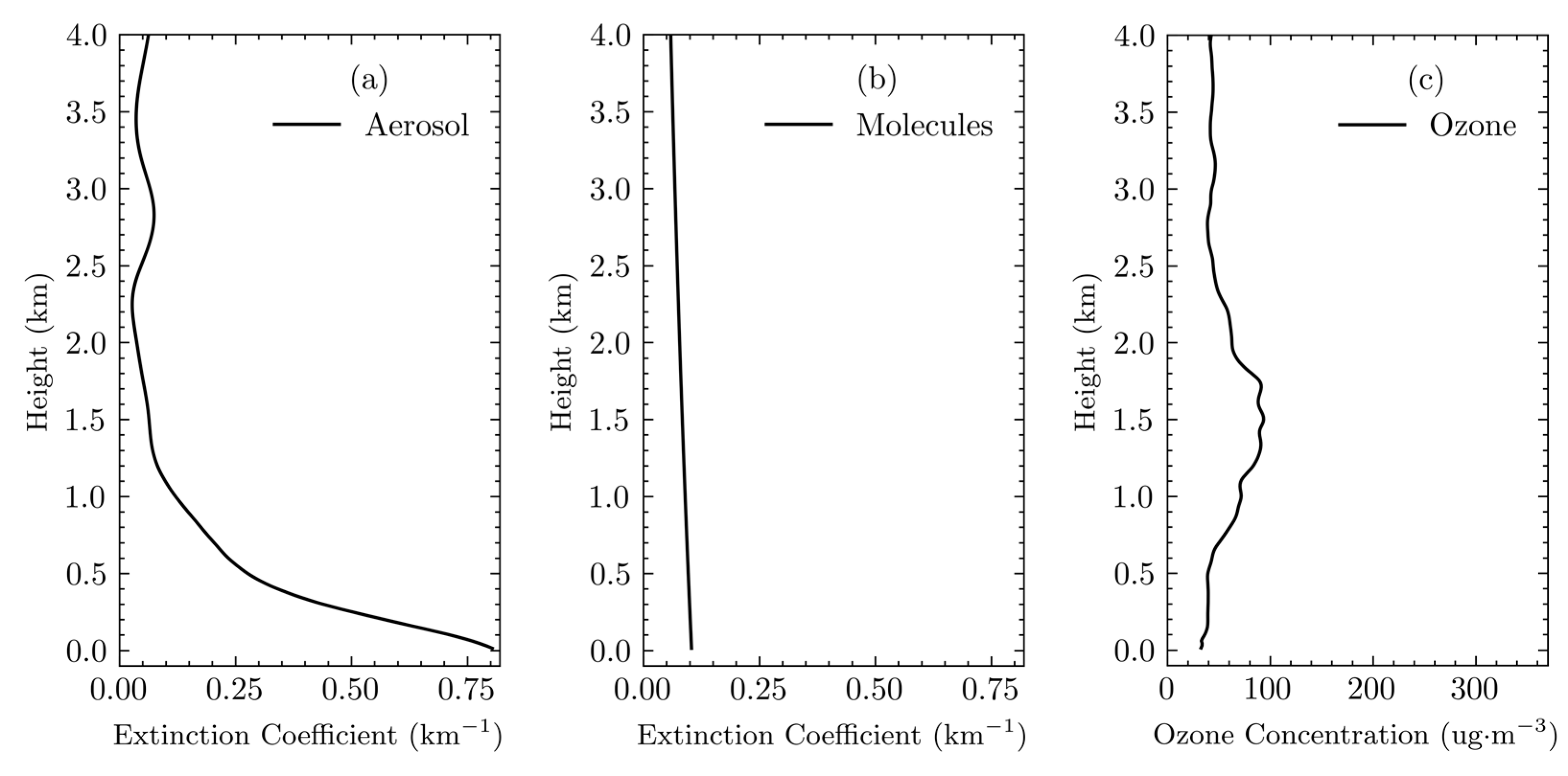
Figure 1 illustrates the basic atmospheric environment established for the simulations in this section, where Figure 1a displays the aerosol extinction coefficient profile at 316 nm as set; Figure 1b shows the extinction coefficient profile for air molecules at 316 nm; and Figure 1c outlines the set atmospheric ozone concentration profile.

The aerosol extinction coefficients and ozone concentrations set in this section are slightly modified based on actual measurement data, whereas the extinction coefficients for atmospheric air molecules are provided by the model (USSA-76). It is generally considered that the atmospheric air molecule model closely fits the real situation, and the errors caused by atmospheric air molecules can be effectively eliminated. The setting of the atmospheric aerosol extinction coefficient highlights the higher concentration of aerosols near the ground surface, with a rapid decrease in the aerosol extinction coefficient with increasing altitude. In this profile, the change in the aerosol extinction coefficient is not completely smooth; some abrupt structural changes are set at 0.5 km, 1.2 km, and 2.3 km to better understand the composition and magnitude of the ozone inversion error at the points of the aerosol structure change.

3. Simulation Results

This section first simulates the various errors of atmospheric disturbance terms in the differential absorption algorithm, analyzing their causes and proportions. Secondly, it analyzes the sensitivity of the two correction methods to aerosol parameters. Finally, considering the inevitable noise issues in actual detection, it compares the ozone inversion accuracy of the two correction methods under different atmospheric conditions. In the simulation process of this paper, the wavelength pair used is 266–316 nm. During the correction process using the triple-wavelength double-differential method, the signal at 289 nm is added.

3.1. Error Analysis of Atmospheric Interference Terms

When retrieving ozone concentration using the dual-wavelength differential absorption algorithm, errors related to the extinction terms of aerosols, atmospheric air molecules, and backscattering terms occur, collectively referred to as errors of atmospheric interference terms. Initially, the causes and proportions of these three errors are analyzed.

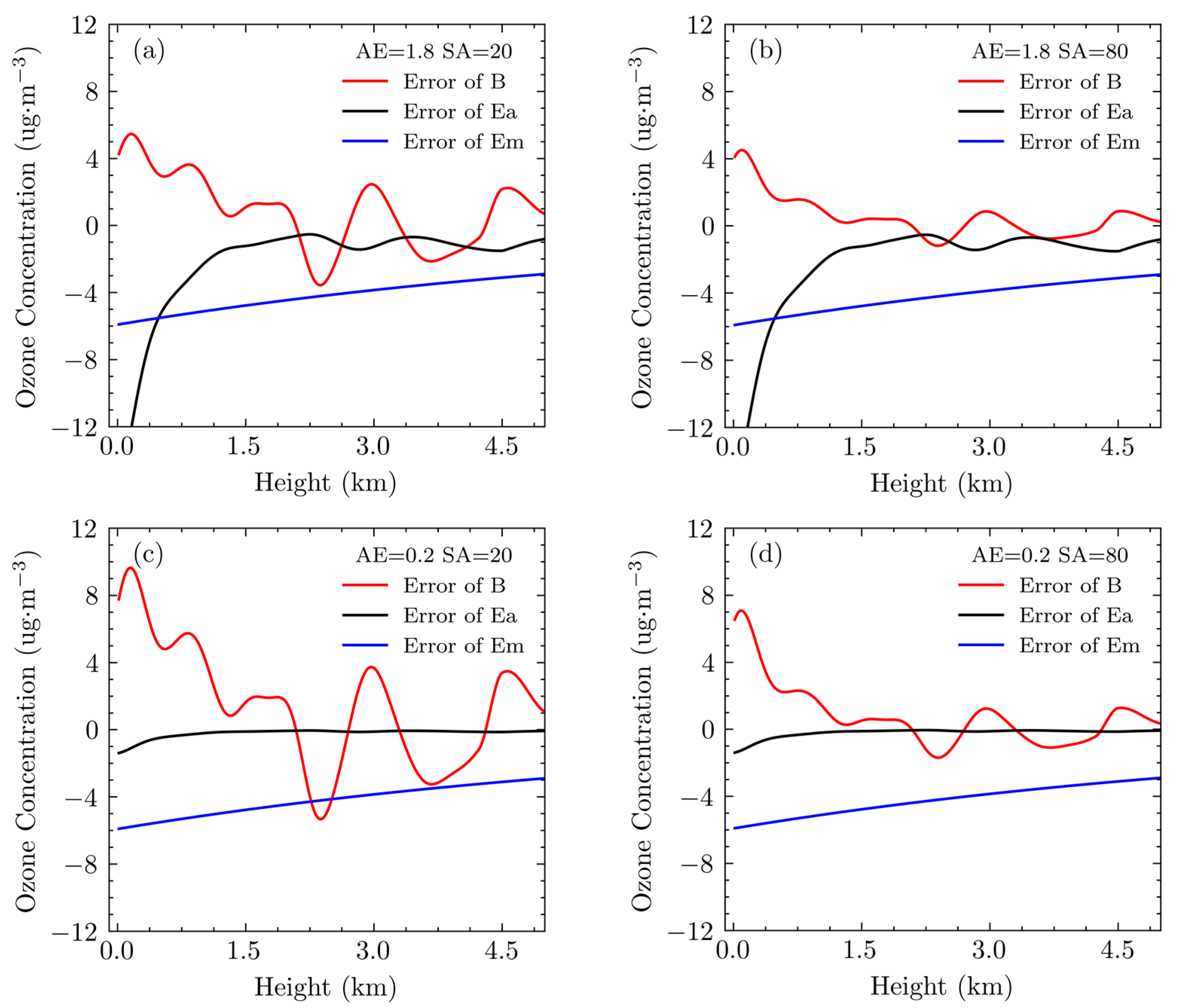
Figure 2 presents the error of atmospheric interference terms under different aerosol backscatter ratio ${(S}_a)$ and Ångström exponent $\left(\delta \right)$, where the aerosol backscatter ratio is denoted as SA and the Ångström exponent as AE in the figure. Since the extinction by atmospheric air molecules is calculated using model data, the error associated with the atmospheric air molecule term remains constant. The error in the aerosol extinction term is directly related to aerosol concentration. When the height is greater than 2 km, where the aerosol concentration is low, the error in the aerosol extinction term is minimal. Compared to the aerosol backscatter ratio, the error in the aerosol extinction term is more sensitive to the Ångström exponent. The closer the Ångström exponent is to 0, meaning the closer the aerosol extinction coefficients are between different wavelengths, the smaller the error in the aerosol extinction term becomes. Overall, the error in the backscattering term also decreases with a decrease in aerosol concentration. However, in areas where aerosol structure changes, such as the 2–3 km region, the error in the backscattering term increases. In regions with higher aerosol concentration, the error in the aerosol extinction term dominates; when the aerosol concentration decreases and is at a point of aerosol structure change, the error in the backscattering term increases and becomes dominant.

3.2. Sensitivity Analysis of Aerosol Parameters

This section will discuss the sensitivity of the ozone inversion errors obtained by the two ozone inversion correction methods described in Section 2.1 to aerosol parameters.

3.2.1. Sensitivity Analysis of Direct Correction

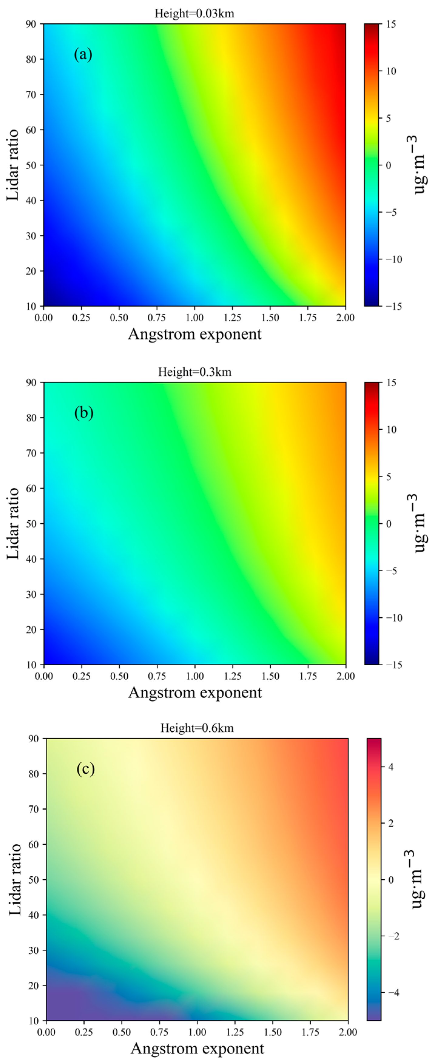
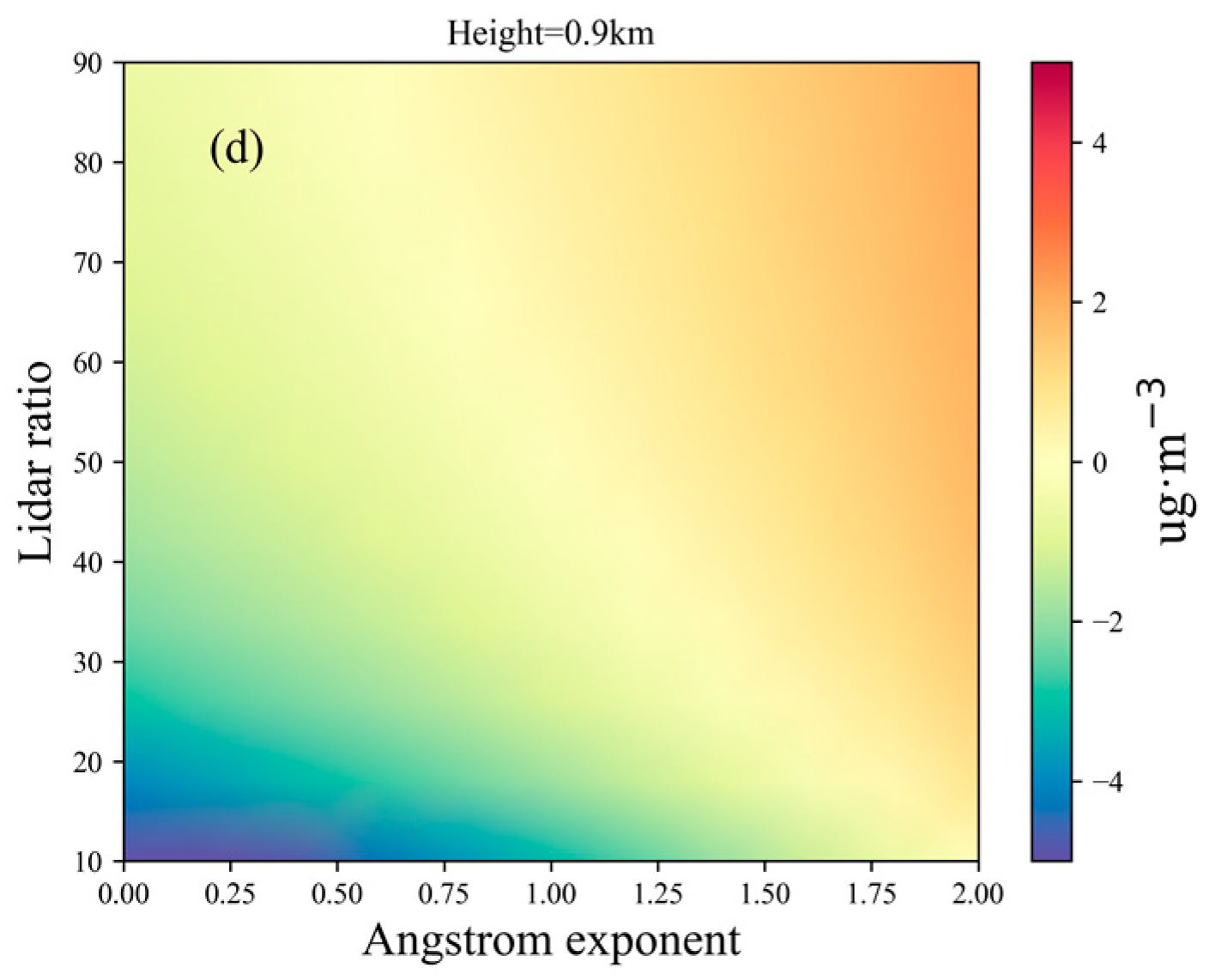
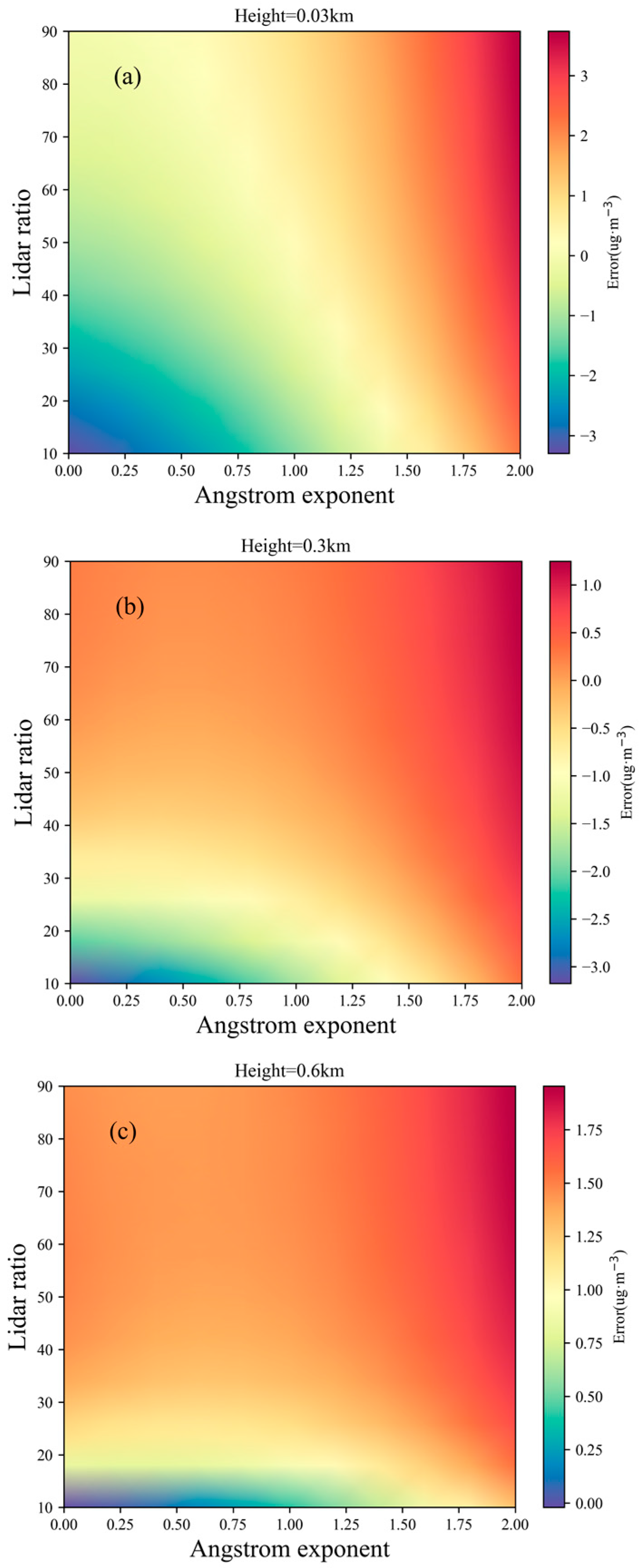
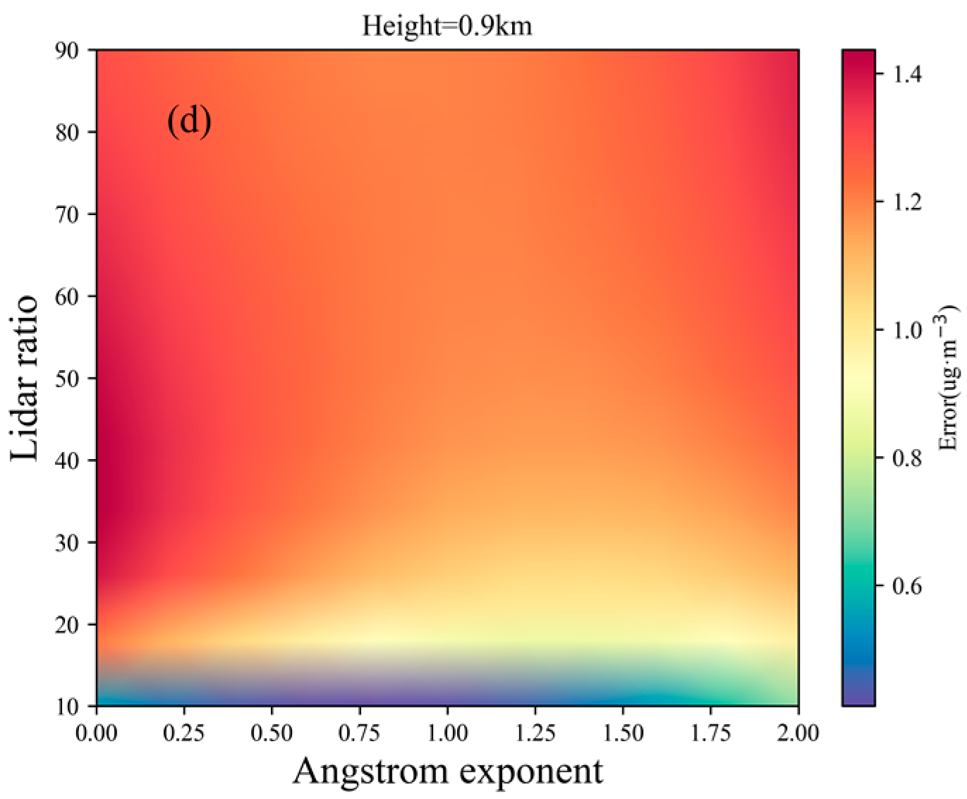
The variation of ozone concentration error with aerosol backscatter ratio and Ångström exponent at different heights is illustrated in Figure 3. The Ångström exponent (AE) varies between 0 and 2, and the lidar ratio (SA) changes between 10 and 90. It is observed that at different heights, there is a certain pattern in the error of ozone inversion. Negative maximum inversion errors occur when the Ångström exponent and lidar ratio are close to 0 and 10, respectively; positive maximum inversion errors appear when they are close to 2 and 90, respectively. Furthermore, it is noteworthy that the direct corrected dual-wavelength algorithm exhibits higher sensitivity to variations in the Ångström exponent.

As depicted in Figure 3a,b, the aerosol extinction coefficient at 316 nm is measured as 0.76 km⁻¹ and 0.43 km⁻¹ at heights of 0.03 km and 0.3 km, respectively, wherein the direct correction dual-wavelength method may exhibit an ozone concentration inversion error exceeding 15 μg/m³. As illustrated in Figure 3c,d, the aerosol extinction coefficient at 316 nm is 0.21 km⁻¹ and 0.18 km⁻¹ at heights of 0.03 km and 0.3 km, respectively, with the ozone inversion error being within 5 μg/m³.

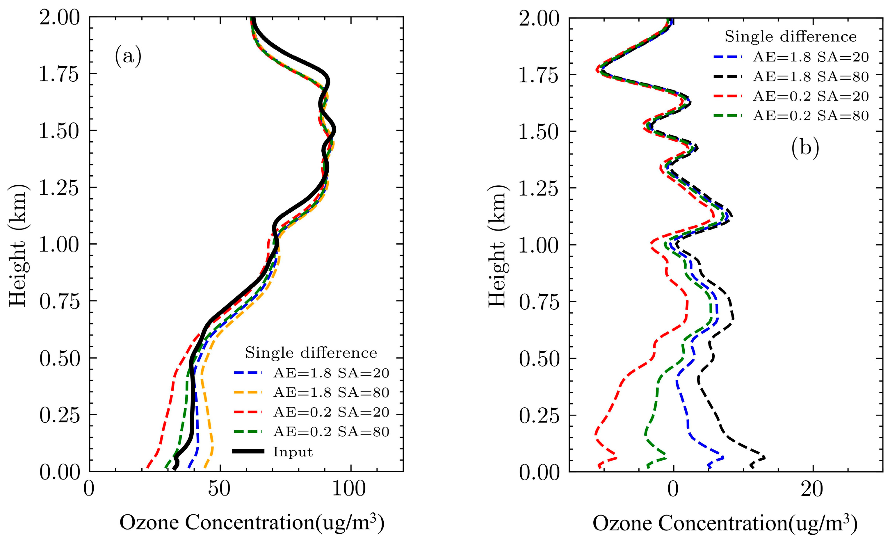
By selecting the Ångström exponent values of 0.2 and 1.8 and lidar ratios of 20 and 80, four sets of ozone concentration inversion profiles and their error curves are obtained. In Figure 4a, the black line represents the set ozone concentration, and the dash-dot lines represent several inversion profiles from the direct correction inversion algorithm. Figure 4b shows their error curves, with the four error curves exhibiting similar structures. Below 1 km, where the aerosol extinction coefficient is larger, the inversion error is greater. The farther the parameters of the error curves deviate from the correction parameters (AE = 1, SA = 50), the greater the ozone inversion error. As altitude increases and aerosol concentration decreases, the inversion results tend to converge.

3.2.2. Sensitivity Analysis of Dual-DIAL Correction

The triple-wavelength double-differential correction, through the processing of two sets of differential results, has mitigated some of the effects caused by aerosols. This subsection analyzes the variation in inversion error of this correction method with the aerosol backscatter ratio and Ångström exponent and presents the ozone inversion and error profiles derived from the triple-wavelength algorithm.

As illustrated in Figure 5, while varying the aerosol backscatter ratio (SA) and Ångström exponent (AE) to simulate the variation in real aerosol parameters, the inversion error from the triple-wavelength double-differential correction does not exhibit a clear pattern with respect to the Ångström exponent and lidar ratio, unlike the direct correction method. The triple-wavelength double-differential correction effectively reduces the influence of aerosols. At an altitude of 0.03 km with an aerosol extinction coefficient (at 316 nm) of 0.76 km⁻¹, the inversion error from the triple-wavelength double-differential correction is within 4 µg/m³, whereas the direct correction error can reach 15–18 µg/m³. At an altitude of 0.3 km, with an aerosol extinction coefficient (at 316 nm) of 0.43 km⁻¹, the inversion error for ozone is already within 3 µg/m³. At altitudes of 0.6 km and 0.9 km, the error from the triple-wavelength double-differential correction is also smaller than that from the direct correction method.

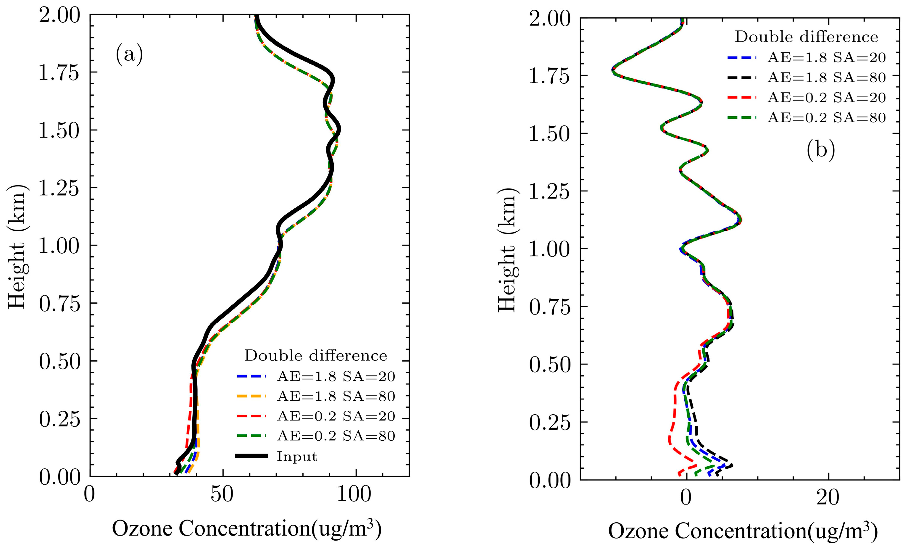
Selecting aerosol backscatter ratios of 20 and 80 and Ångström exponents of 0.2 and 1.8, four sets of ozone concentration inversion profiles and error curves are obtained through the triple-wavelength double-differential correction. In Figure 6a, the black line represents the preset ozone concentration, while the dash–dot lines are several inversion profiles from the triple-wavelength double-differential correction. Figure 6b displays the corresponding error curves. The four error curves have similar structures, but their relationship with aerosol parameters is not clear.

3.3. Comparison of Algorithm Performance under Noise Conditions

In the actual detection process, the interference of noise is inevitable. Noise affects the performance of lidar and the accuracy of measurement results, directly impacting measurement precision and system performance. Incorporating noise factors into simulation design can enhance the accuracy and reliability of the simulation, providing a better understanding of the challenges and limitations the system may face in actual operation and making the simulation results more closely aligned with real-world conditions. Evaluating the impact of noise on system performance allows for a more accurate prediction of the system’s behavior under real conditions. Studying the impact of noise on signal processing aims to improve the quality of the signal and the overall performance of the system.

In differential absorption lidar systems, noise sources can be divided into background light noise $N_b\left(\mathsf{\lambda },z\right)$ and detector noise $Nd\left(\mathsf{\lambda },z\right)$. The background light noise, originating from solar radiation or other artificial light sources, can enter the detector through the optical components of the receiving system and mix with the signal light, leading to noise. Detector noise includes thermal noise, shot noise, dark current noise, etc., all of which are generated internally by the detector. Among these, shot noise, which is related to the number of photons detected, is a manifestation of quantum noise. These two types of noise can be expressed by the following Equations:

$$N_b\left(\mathsf{\lambda }\right)=\frac{\eta \left(\mathsf{\lambda }\right)\mathsf{\lambda }}{hc}{P}_b(\mathsf{\lambda })\mathsf{\pi }\frac{\theta }{2}\mathsf{\Delta }\mathsf{\lambda }(\mathsf{\lambda })A_r{T}_r\Delta t$$

(10)

$$N_d\left(\mathsf{\lambda }\right)=C_{PS}\left(\mathsf{\lambda }\right)\mathsf{\Delta }t$$

(11)

$P_b\left(\mathsf{\lambda }\right)$ is defined as the sky background radiance at wavelength $\mathsf{\lambda }$. At night, this value is close to 0; thus, operating a DIAL system at night can significantly reduce the impact of background light noise. θ is the receiving field of view angle of the receiving telescope; Δλ(λ) is the half-width of the spectral device at wavelength λ; $T_r$ is the transmittance of the receiving optical unit at wavelength λ, and $C_{PS}\left(\mathsf{\lambda }\right)$ is the dark count of the detector. The signal-to-noise ratio SNR(λ,z) of the atmospheric backscatter signal from the differential absorption lidar can be calculated using the formula below:

$$SNR\left(\mathsf{\lambda },\mathrm{Z}\right)=\frac{N_{\mathrm{s}}\left(\mathsf{\lambda },\mathrm{Z}\right)}{\sqrt{N_s\left(\mathsf{\lambda },\mathrm{Z}\right)+{2(N}_b\left(\mathsf{\lambda },\mathrm{Z}\right)+N_d\left(\mathsf{\lambda },\mathrm{Z}\right))}}\sqrt{M}$$

(12)

where M is the number of pulses.

Combining the parameters from the table above simulates the atmospheric transmission process in the air. Introduce noise into the lidar equation. Calculate the echo signals at 266 nm, 289 nm, and 316 nm.

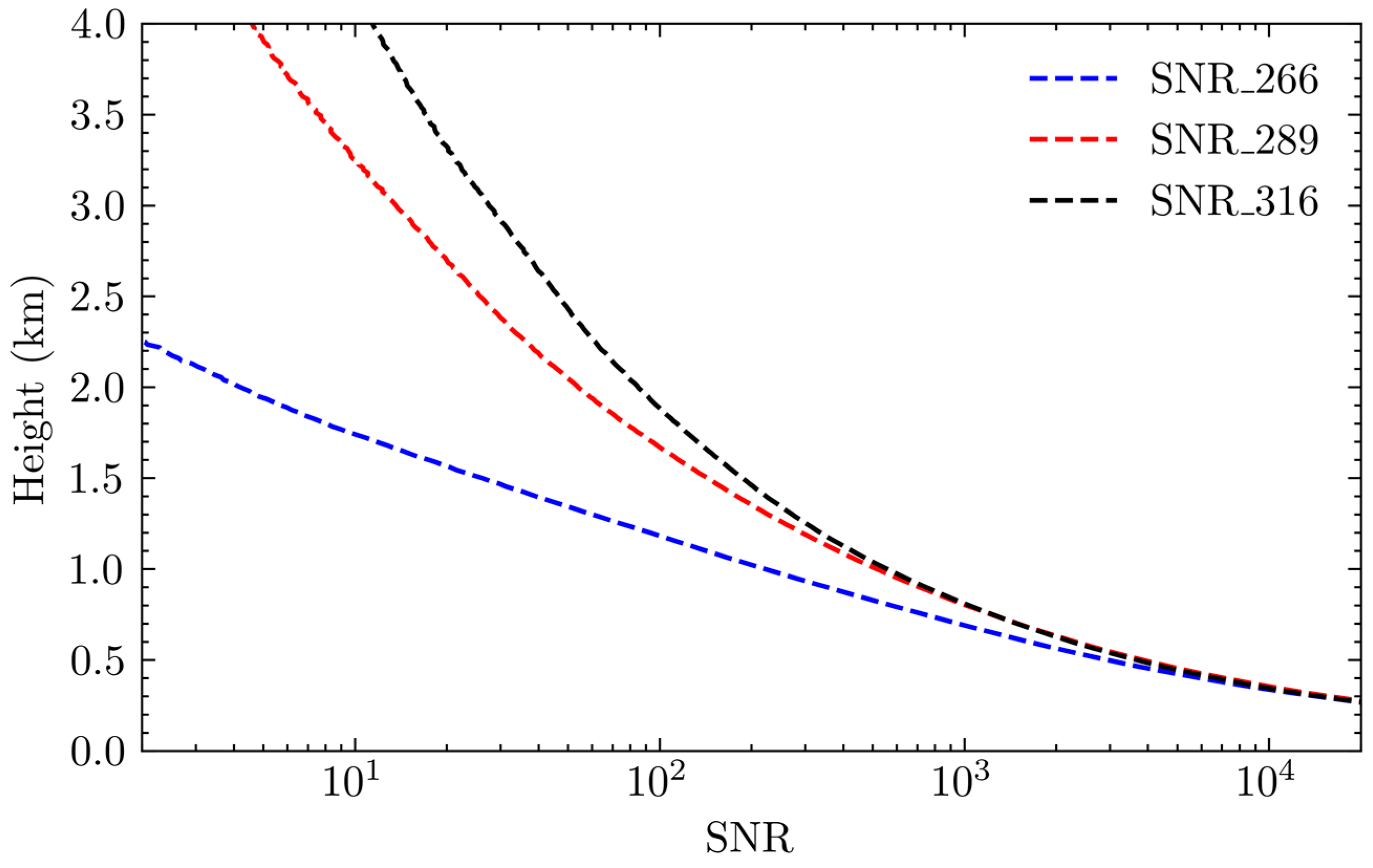
The signal-to-noise ratio (SNR) for the three wavelengths is obtained by substituting the echo signals into the SNR formula, as shown in Figure 7. The detection altitudes for 266 nm, 289 nm, and 316 nm, where the SNR is 10, are respectively 1.725 km, 3.18 km, and 4.09 km. In the ultraviolet spectrum, as the wavelength decreases, the atmospheric backscatter effect intensifies, leading to a faster attenuation of signal strength. Therefore, there are significant differences in the effective detection distances among the signals at the three different wavelengths. Within these effective detection ranges, the variation in the echo signals across the three wavelengths can reach up to five orders of magnitude.

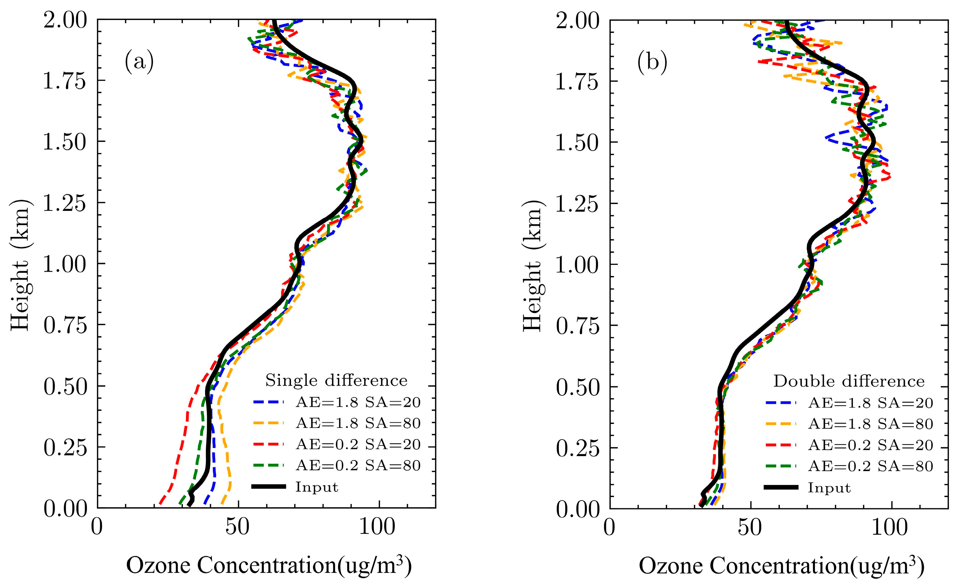
Under the lidar system parameters listed in

Table 1. Simulated Lidar Parameters for Calculation.

System Parameter	Value
Laser wavelength	266 nm, 289 nm, 316 nm
Pulse energy	1 mJ
Pulse number	700
Emitting optical transmittance	0.3
Detection Quantum Efficiency	0.2
Receiver Diameter	300 mm
Field of view	1 mrad
Filter Bandwidth	1 nm
Dark counts	400
Spatial resolution	7.5 m

, by varying the aerosol backscatter ratio and Ångström exponent, ozone concentration profiles were retrieved through both direct correction and Dual-DIAL correction, as shown in Figure 8. Figure 8a presents the results from direct correction, and Figure 8b from the Dual-DIAL correction. The inversion spatial resolution was set at 60 m. In high signal-to-noise ratio (SNR) areas (such as below 1 km), the ozone profiles are essentially consistent with the ideal state (in the absence of noise); as the SNR of the wavelength signal decreases, fluctuations appear in the inverted ozone concentration.

The results depicted in Figure 8 demonstrate the efficacy of employing a Dual-DIAL correction in mitigating aerosol-induced influences; however, it necessitates a higher signal-to-noise ratio, as evident from the findings.

4. Error Caused by Noise

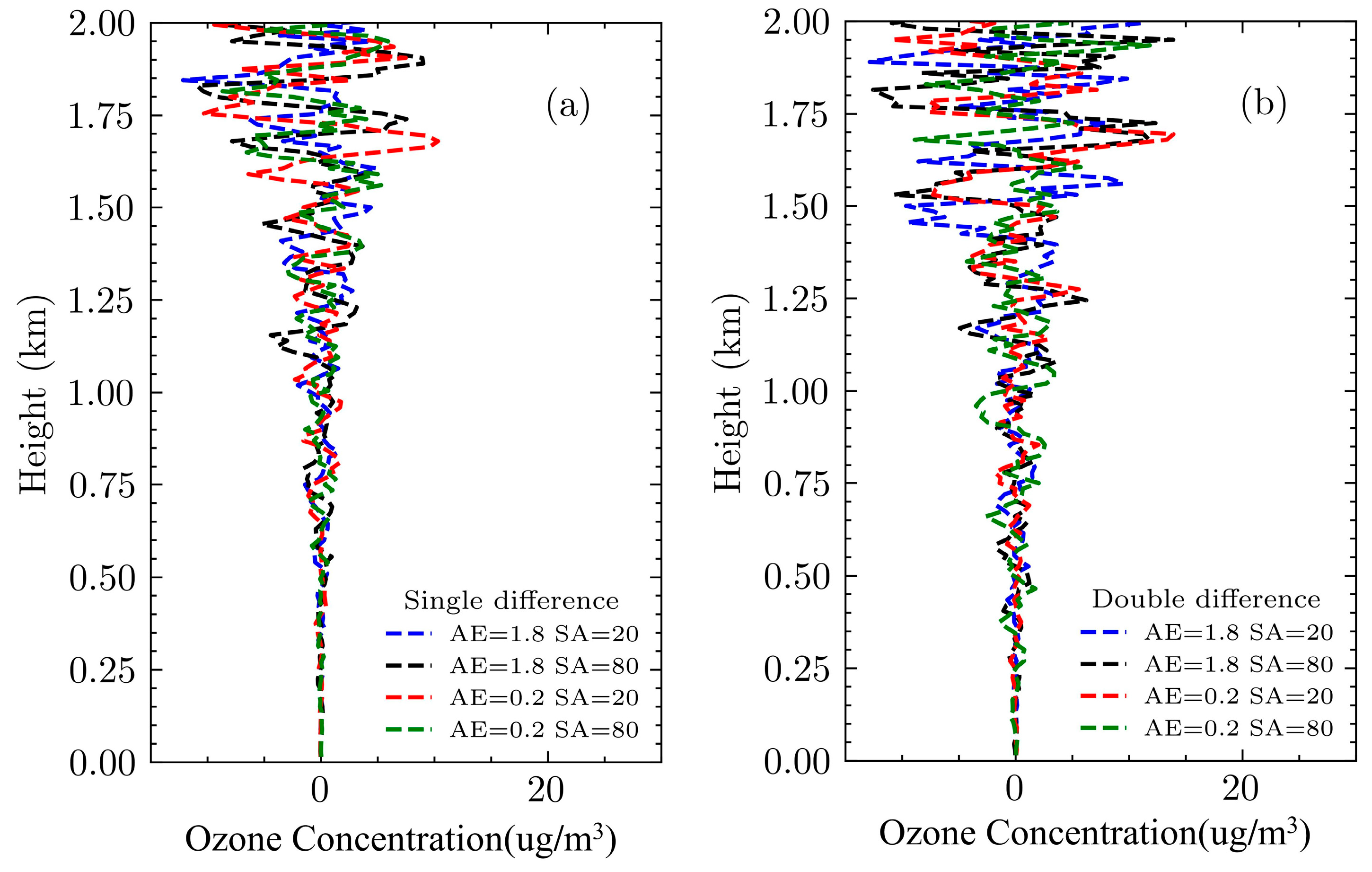
The error in Figure 8 can be divided into two parts: one part is the error caused by the interference of aerosols, and the other part is the error generated by system noise. By comparing with the ozone inversion profile under ideal conditions, the magnitude of errors caused solely by noise for both algorithms can be obtained, as shown in Figure 9.

Figure 9a shows the error caused by noise in direct correction, while Figure 9b shows the error caused by noise in Dual-DIAL correction. It is observed that when the error reaches 5 µg/m³, the inversion heights for direct correction and Dual-DIAL correction are 1.3 km and 0.8 km, respectively. When the inversion height reaches 2 km, the errors caused by noise in direct correction and Dual-DIAL correction are 8 µg/m³ and 15 µg/m³, respectively.

Combining Figure 8 and Figure 9, it can be seen that in the high-concentration aerosol areas near the ground, the Dual-DIAL correction performs better, as it can reduce most of the aerosol interference. As the altitude increases and the lidar signal’s signal-to-noise ratio becomes insufficient, the direct correction method is less affected by noise and yields better inversion results. From this, we can conclude the following strategy for actual detection: use the Dual-DIAL correction in areas of high aerosol concentration and the direct correction method in areas of low aerosol concentration. This inversion strategy can effectively improve the accuracy of ozone inversion and the detection distance of ozone.

5. Discussion

Studying the distribution of atmospheric ozone concentration in the troposphere is of significant importance for understanding atmospheric chemistry, assessing environmental impacts, and studying climate change. Compared to other detection methods, differential absorption lidar (DIAL) exhibits unique advantages in detecting ozone concentration distribution, including high-resolution vertical profiles, high temporal and spatial resolution, multi-parameter measurement capabilities, high sensitivity, and long-range detection. These advantages make lidar a powerful tool for researching and monitoring ozone distribution.

From a theoretical algorithm perspective, the main challenge of using DIAL for detecting ozone concentration distribution lies in the interference from atmospheric aerosols. In traditional inversion algorithms, the wavelength dependence of aerosol extinction on laser radiation is unknown, and it is mistakenly calculated as ozone concentration. Particularly in the region from near the surface to the troposphere, on the one hand, the ozone concentration in the troposphere is relatively low compared to the stratosphere, and on the other hand, anthropogenic activities and industrial production contribute to higher aerosol content in the atmosphere in this region.

In order to mitigate the impact of aerosols on the DIAL algorithm, the current mainstream research directions can be divided into two categories. One approach does not focus on the optical properties of aerosols along the laser path but instead aims to compensate for or reduce atmospheric interference through experimental methods.

For example, McGee utilized the backscattered signal of the receiving laser on nitrogen molecules to obtain ozone concentration profiles under high aerosol concentrations. It is widely recognized that this method effectively eliminates the influence of aerosol backscattering error. However, errors in aerosol extinction still persist [27]. Wang et al. proposed a three-wavelength dual differential absorption lidar technique and used a three-wavelength dual-wavelength lidar system to detect ozone in the stratospheric region after a volcanic eruption [29]. Su et al. conducted monitoring of the lower atmospheric vertical profile in the urban area of Hangzhou using a three-wavelength dual differential absorption algorithm and compared the results with measurements obtained from radiosonde balloons [32]. Yang et al. simulated the production and diffusion process of ozone, evaluated the performance of ozone concentration inversion using a multi-wavelength DIAL system, and conducted verification in the Chengdu region of China [33].

Another approach involves detecting the optical properties of aerosols along the laser path through other means to correct the inverted ozone concentration. For example, Ma et al. analyzed the atmospheric backscattering signals at three wavelengths, 266 nm, 289 nm, and 316 nm, to obtain ozone concentrations. They then used the backscattered signal at 532 nm to correct for the aerosol optical effects [34]. Lei et al. studied the impact of aerosols emitted from wildfires on ozone concentration inversion using Differential Absorption Lidar. They obtained aerosol extinction coefficients at 532 nm and 292 nm through different methods and determined the Ångström exponent of the aerosols to correct for their influence [35]. Kuang et al. utilized a High Spectral Resolution Lidar (HSRL) to retrieve the aerosol extinction coefficients at 532 nm and 340 nm. They combined the backscattered signals from the DIAL to invert the aerosol extinction coefficient profiles and Ångström exponent and subsequently corrected the ozone concentration [36].

These two research directions provide important references for accurately inverting ozone concentrations in the atmosphere. However, they also have some unresolved limitations. Correcting the ozone concentration using experimental methods can theoretically only remove a portion of the aerosol influence and impose higher requirements on the signal-to-noise ratio(SNR) of the lidar signals. On the other hand, the other research direction is evolving towards joint inversion of aerosol and ozone concentrations. However, it faces the challenge that the state of aerosols cannot be precisely determined, leading to uncertainties in correcting the ozone concentration.

Based on the aforementioned background, this study delves into the mechanisms of aerosol impact on ozone concentration inversion. By combining predefined atmospheric conditions and lidar parameters, the inversion effects of different correction methods are simulated and investigated. A novel strategy for differential absorption ozone concentration inversion is proposed. This strategy utilizes a three-wavelength dual differential algorithm for correction under conditions of high aerosol concentrations and high SNR. Conversely, a direct correction method is employed for correction under other conditions. Compared to traditional methods, this strategy offers higher inversion accuracy and longer detection distances.

The work presented in this paper is not specific to any particular lidar system but focuses on analyzing and studying the constraints of the ozone inversion algorithms themselves. The constraints depend on the actual atmospheric conditions and the SNR of the lidar signals. Therefore, it is not necessary to provide specific lidar parameters or quantified boundary conditions.

6. Conclusions

This paper conducts a simulation study on the inversion of ozone concentration using the differential absorption lidar algorithm. Initially, under ideal conditions, the atmospheric interference terms of the differential absorption algorithm are simulated and calculated, analyzing their causes and proportions. Subsequently, a sensitivity analysis of aerosol parameters is performed for both direct correction and triple-wavelength double-differential correction. Finally, considering the inevitable noise issues in actual detection, the inversion accuracy of these two correction methods under different atmospheric conditions is compared. A better inversion strategy is proposed.

The simulation results indicate the following:

For the atmospheric interference terms of the differential absorption algorithm, the error caused by aerosol extinction dominates under conditions of higher aerosol concentration and stable aerosol structural changes. In contrast, the error caused by backscattering dominates under conditions of lower aerosol concentration and changing aerosol structure.

Compared to the aerosol backscatter ratio, the ozone concentration inversion error obtained through direct correction is more sensitive to the aerosol’s Ångström exponent. However, the sensitivity of the ozone concentration inversion error from triple-wavelength double-differential correction to these two parameters does not exhibit a clear pattern. In the absence of noise, triple-wavelength double-differential correction can better reduce the impact of aerosols on ozone concentration inversion.

Considering the inevitable noise issues in actual detection and adjusting aerosol parameters, a simulation analysis of the ozone concentration inversion error for both correction methods was conducted. In areas of high SNR and high aerosol concentration, the inversion accuracy of both correction methods is close to the ideal state, with the triple-wavelength double-differential correction achieving higher ozone concentration inversion accuracy. With increasing height, both SNR and aerosol concentration decrease, leading to dominant errors induced by noise and consequently resulting in improved inversion accuracy when employing the direct correction method.

In summary, the triple-wavelength double-differential correction method can be used in areas with high SNR and high aerosol concentration, while the direct correction method is suitable for areas with low SNR and low aerosol concentration. This strategy for ozone concentration inversion enables enhanced accuracy and an extended range of inversion.