Article

Deep Learning-Enhanced Inverse Modeling of Terahertz Metasurface Based on a Convolutional Neural Network Technique

1
College of Control Science and Engineering, China University of Petroleum, Qingdao 266580, China
2
College of Electronic and Information Engineering, Shandong University of Science and Technology, Qingdao 266590, China
*
Author to whom correspondence should be addressed.
Photonics 2024, 11(5), 424; https://doi.org/10.3390/photonics11050424
Submission received: 30 March 2024 / Revised: 27 April 2024 / Accepted: 28 April 2024 / Published: 3 May 2024
(This article belongs to the Special Issue Fiber Optic Sensors: Science and Applications)

Abstract

:
The traditional design method for terahertz metasurface biosensors is cumbersome and time-consuming, requires expertise, and often leads to significant discrepancies between expected and actual values. This paper presents a novel approach for the fast, efficient, and convenient inverse design of THz metasurface sensors, leveraging convolutional neural network techniques based on deep learning. During the model training process, the magnitude data of the scattering parameters collected from the numerical simulation of the THz metasurface served as features, paired with corresponding surface structure matrices as labels to form the training dataset. During the validation process, the thoroughly trained model precisely predicted the expected surface structure matrix of a THz metasurface. The results demonstrate that the proposed algorithm realizes time-saving, high-efficiency, and high-precision inversion methods without complicated data preprocessing and additional optimization algorithms. Therefore, deep learning algorithms offer a novel approach for swiftly designing and optimizing THz metasurface sensors in biomedical detection, bypassing the complex and specialized design process of electromagnetic devices, and promising extensive prospects for their application in the biomedical field.

1. Introduction

Terahertz (THz) waves, renowned for their non-invasive nature and sensitivity to biomolecules, present promising opportunities for biological detection [1,2]. However, challenges arise from their weak interaction with diluted biological samples. THz metasurfaces, characterized by microscale periodic structures with distinctive electromagnetic properties, offer effective solutions, including high-resolution imaging and rapid detection [3,4,5,6,7]. In the realm of biomedical science, these metasurfaces hold vast potential for advancing diagnostic and therapeutic technologies [8,9].
Researchers have extensively studied THz metasurfaces for their potential applications in biosensing. Traditional methods for designing THz metasurfaces primarily involve equivalent circuit theory, electromagnetic wave theory, and parameter sweeping optimization algorithms. Rishi Mishra et al. proposed an approach based on equivalent circuit models to design frequency-selective graphene-based metamaterial absorbers for the THz band [10]. Xiaofeng Liu et al. designed THz electromagnetically induced transparency metamaterials using electromagnetic theory [11]. Additionally, Rustam R. Gaynutdinov et al. presented a method using artificial bee colony optimization algorithms to determine optimal component parameters for creating electromagnetic shielding layers with specific reflection and transmission coefficients [12]. In summary, traditional THz metasurface design methods are characterized by high specialization, repetition, and time consumption, relying on theoretical frameworks limited to conventional metasurface structures. Consequently, obtaining solutions for unconventional structures using traditional methods can be challenging.
To address traditional electromagnetic device design limitations, scholars have turned to neural networks (NNs). Qiu et al. proposed an automatic microwave metasurface design method using autoencoders. By utilizing preprocessed EM characteristic curves for structure prediction, an average accuracy of 76.5% was achieved [13]. Shi et al. utilized autoencoders and artificial bee colony optimization for microwave metasurface design [14]. Pal et al. applied an NN to optimize the parameters of complementary split-ring resonators [15]. In summary, the NN models employed in these studies are either shallow, requiring complex preprocessing techniques and optimization algorithms for improved predictive performance, or specifically tailored for electromagnetic devices in the microwave band, with investigation into metasurface plasma characteristics in the THz band lacking in these studies. Considering the vast application potential of THz metasurface sensors in bio-detection, the utilization of deep NN algorithms for THz metasurface inverse design holds promising prospects.
Based on the limitations of traditional THz metasurface design methods and the advantages of NNs in the field of electromagnetic device design, this paper proposes a novel method for the inverse design of THz metasurface device surface structures. In this work, we employ a deep one-dimensional convolutional neural network (1D-CNN) combined with an adaptive moment estimation (Adam) for the inverse design of THz metasurface structures. During training, the S-parameter magnitude data of the THz metasurface served as inputs, with its matrices as corresponding outputs, facilitating continuous learning of the mapping relationship between them. In the validation process, the model accurately predicted THz metasurface structures without requiring extra preprocessing or optimization steps. From the final results, it can be observed that the proposed design method for THz metasurface structures in this work not only simplifies the entire design process compared to traditional methods, eliminating the need for additional data preprocessing steps, but also has the advantages of being time-saving and efficient, with significant improvements in design accuracy. Designing THz metasurfaces will no longer be limited by the lack of electromagnetic engineering research experience, as the method proposed in this work lowers the design threshold. The THz metasurfaces designed using the method proposed in this work serve as specialized detection tools in the biosensing field. They offer a convenient approach to designing biosensors tailored to meet specific biosensing requirements, showcasing broad applications in both biological studies and detection technologies.

2. Theory and Methodology

This paper introduces an inverse design methodology for THz metasurface sensors utilizing deep learning (DL) algorithms. Since this technology combines two different areas of research, namely THz metasurface sensors and DL techniques, this section provides a brief overview of the basic theories and methods in these areas to improve the clarity of our technology principles. In addition, this section also describes the method used to generate the dataset.

2.1. THz Metasurface Sensor and Resonant Characteristics

Scattering parameters (S-parameters) are usually employed to describe the EM characteristics of metasurfaces, holding substantial importance in the design and utilization of metasurfaces [16]. The concept of the S-parameter is related to the energy flow. S11 and S21 represent the reflection or transmission characteristics caused by the impedance matching of the network, respectively. The analysis of S-parameter frequency response curves allows a more profound comprehension of the EM response mechanisms within metasurfaces.
Figure 1a shows a metasurface resonator, which is a typical rectangular split-ring resonator (SRR) structure with gaps at symmetric positions along the metallic rings [17,18]. The entire model consists of only two layers: the substrate and the metallic layer. Figure 1b depicts its corresponding S-parameter curve. Given the restricted penetration of THz waves and the thinness of the substrate in the THz band, flexible and highly transparent materials such as polyethylene terephthalate or polyimide are typically chosen as substrate materials. Additionally, owing to the limitations of micro–nano fabrication technology, the SRR structure on the substrate surface is commonly crafted from gold.
When EM waves interact with the SRR structure, the metallic components and gaps induce noticeable oscillations or peaks in the S-parameters at specific frequencies, a phenomenon referred to as the resonance characteristic [19]. Resonance arises due to the SRR’s equivalence to an LC resonance circuit, with a fixed resonance frequency determined by the geometry and material properties of the structure. When the frequency of the electromagnetic wave matches the resonance frequency of the metasurface, resonance occurs. The resonance phenomenon amplifies the electric and magnetic fields within the metasurface, leading to enhanced interaction with electromagnetic waves at specific frequencies. In the process of biomolecular detection and analysis with the SRR, the existence of the substance to be detected will cause the electrical characteristics of the SRR surface to change and then cause the change in the resonant curve. By leveraging the alterations in resonant features exhibited by biological resonant sensors, including shifts in frequency and variations in peak depth, in conjunction with pertinent analytical techniques, it becomes feasible to ascertain various biological properties of the target, spanning from its structural attributes to its compositional makeup [20,21].
THz metasurfaces can be manufactured using techniques akin to nanofabrication [22]. These techniques involve lithography for defining subwavelength patterns, etching for pattern transfer onto substrates, and deposition methods like sputtering or evaporation for material fabrication. Characterization techniques are then used to evaluate the metasurface performance and properties [23]. Overall, the fabrication process emphasizes precision and control at the microscale to achieve the desired electromagnetic properties, aligning with optical device manufacturing principles.

2.2. Deep Learning Algorithms

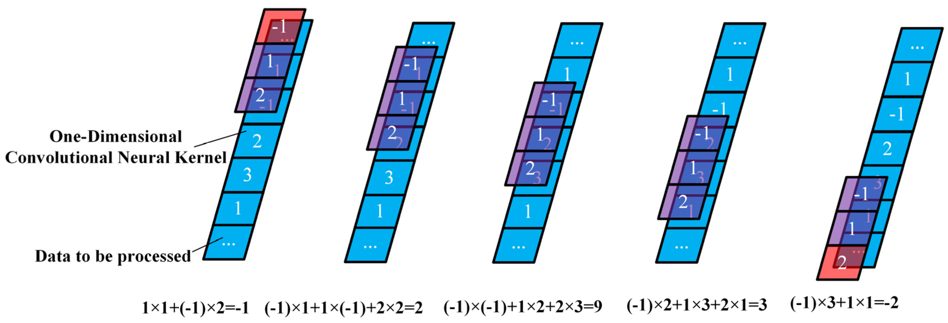
The CNN, as a variant derived from conventional NNs, offers a diverse set of functional NNs [24]. As the name suggests, 1D-CNNs are commonly employed for processing curve data [25,26]. They operate in a single direction, as illustrated in Figure 2. One-dimensional convolution effectively captures local patterns and dependencies in sequential data, making it ideal for time-series or one-dimensional signal tasks. Therefore, this work aims to utilize a 1D-CNN to capture the reflection relationship between the one-dimensional S-parameter curves and metasurface sensor structures.
Each layer of the NN contains numerous neurons, and the output of neurons in the previous layer serves as the input to neurons in the next layer. Through successive layers, specific mapping relationships are formed between pairs of neurons, which can be represented by Equation (1). Here, w, b, and f represent the weight, bias, and activation function, respectively.
y = f ( w x i + b i )
The presence of activation functions introduces non-linearities, enabling NNs to learn complex patterns and relationships in data [27]. When a neuron receives the weighted sum from the neurons in the preceding layer, it undergoes activation functions such as the rectified linear unit (ReLU) and the logistic function (Sigmoid), as shown in Equations (2) and (3). The Sigmoid activation function, which is ideal for binary classification tasks, ensures output normalization between 0 and 1 and provides a smooth gradient across the input domain. However, it encounters challenges such as the vanishing gradient problem, particularly for extreme inputs, and computational inefficiency due to exponentiation. The ReLU activation function is introduced as a solution for training DL networks, addressing the issue of vanishing gradients encountered with Sigmoid functions. While ReLU effectively mitigates vanishing gradient problems, it is prone to the “dying ReLU” phenomenon, where neurons may deactivate for negative inputs, resulting in stagnant gradients and slower learning in specific contexts.
f ( x ) = max ( 0 , x )
f ( x ) = 1 1 + e x
The loss function serves as a measure for evaluating the discrepancy between the actual and expected values in the NN model [28]. The BCEWithLogitsLoss function, short for Binary Cross-Entropy Loss with Logits, combines the Sigmoid activation function with the Binary Cross-Entropy Loss. It is commonly used for multi-label multi-classification problems, where the model’s output logits are first transformed into probabilities using Sigmoid and then compared with the target labels to compute the loss. The formula is given below, where N represents the number of samples, while zn and yn represent the score predicting the nth sample as positive and the label of the nth sample, respectively.
{ l o s s ( z , y ) = m e a n { l 0 , , l N 1 } l n = ( y n l o g ( s i g m o i d ( z n ) ) + ( 1 y n ) l o g ( 1 s i g m o i d ( z n ) ) )
Two key hyperparameters in NN models are the learning rate (lr) and batch size (batch) [29]. lr influences parameter updates, with large values accelerating training but risking instability, while small values may prolong training. Batch determines the number of samples in each training iteration, where a larger batch expedites training but may lead to overfitting, while a smaller batch promotes generalization but requires more time. A balanced choice of batch and lr is vital for optimizing model performance and avoiding overfitting.

3. Data Collection and Model Construction

The previous section briefly introduced the fundamental theories relevant to the research objectives of this paper. In this section, the THz metasurface sensor structure representation method and the process of data generation will be clarified, and then the construction process of the inversion model will be explained.

3.1. THz Metasurface Sensor Structure Representation and Dataset Generation

To simplify and optimize the representation of THz metasurface sensor structures for processing by DL models, this work utilizes a binary matrix, as illustrated in Figure 3. Each metasurface unit in the metallic layer can be viewed as an 8 × 8 grid array marked with “0” or “1”, where “1” represents the presence of metal at the current position, and “0” represents the absence of metal. Therefore, the surface structure of a THz metasurface sensor can be represented by a binary matrix. Each grid has a side length of 20 μm and is made of glossy gold with a thickness of 0.12 μm. The substrate material chosen is polyimide.
If all 64 positions are to be fully encoded, the required computational resources would be immense, being estimated to be approximately 1.85 × 10¹⁹ scenarios. It is not feasible to conduct simulations and collect data for most scenarios within a realistic timeframe, as this would require billions of years using current computational resources. Therefore, this paper intends to represent the entire model using a quarter of the metasurface structure. On this basis, a complete metasurface sensor model is obtained through symmetrical duplication. This simplifies the structural complexity of the THz metasurface biosensor and also allows for the representation of asymmetric scenarios to some extent. Furthermore, it significantly streamlines the data generation process, particularly for the subsequent training and validation of inversion models. This streamlined design process conserves significant computational resources.
During the dataset generation process, a 4 × 4 binary matrix is randomly generated in commercial mathematical software. The CST STUDIO SUITE 2018 models are based on the distribution of elements in the random matrix. Finally, symmetry operations are applied twice in the X and Y directions to obtain a complete metasurface model. In this way, each metasurface unit can be represented by a 4 × 4 random binary matrix. The 16-dimensional elements of the random matrix serve as labels for the dataset. The S-parameters obtained from simulation after modeling are used as features in the dataset. Other settings include using periodic boundary conditions in the X and Y directions and open boundaries in the Z direction. The simulation frequency range is 0.1–1.1 THz. The Frequency Domain Solver is selected.
To assess the generalization ability of the 1D-CNN for the inversion of THz metasurface sensor structures with different substrate thicknesses (20 μm, 50 μm, and 80 μm), three sets of datasets are generated in this study. Each dataset with varying substrate thickness comprises 7000 pairs of data (random matrix and its corresponding S-parameters). Among them, 6000 pairs of data are used for model training, while the remaining 1000 pairs of data are used for testing the model, which the model does not encounter during training.

3.2. One-Dimensional CNN Inversion Model Construction

This subsection will describe the specific process of constructing the inversion model and illustrate how input data are propagated through the model.
To preserve the fundamental characteristics of the S-parameters while reducing input dimensions, this work performs equidistant sampling on the saved S-parameters as inputs to the inversion model. After simulating a THz metasurface structure, the corresponding S-parameters curve data are saved, where each curve contains 1001 points, serving as input for the inversion model. The inversion model produces a 4 × 4 matrix as the output, resulting in a 16-dimensional output. For the model architecture, a five-convolutional-layer model is considered, with the number of channels ranging from (1, 8) to (64, 96) across the layers. Each convolutional kernel size is set to 3 to comprehensively capture the features of the S-parameters curve, with a stride of 1 to prevent information loss. Moreover, max pooling operations are added after convolutional layers to decrease the parameter count and computational complexity, allowing more salient features to be captured. Subsequently, the data pass through three linear layers with input–output pairs of (256, 128), (128, 64), and (64, 16). ReLU activation functions are applied after each convolutional and fully connected layer to mitigate the gradient vanishing problem, enhancing the model’s expressive power and learning capacity. The Adam optimizer was chosen for its simplicity in implementation, efficient computation, and minimal memory requirements.
During the actual training process, S-parameters (using S11 as an example, with S21 following the same process) are input into the model. Following input, data sequentially traverse all convolutional layers within the network model. After the input passes through all convolutional layers and completes feature extraction, the features captured by each channel are reshaped into a one-dimensional vector to facilitate prediction by subsequent linear layers. Following this dimension adjustment, it then progresses through three fully connected layers before reaching the output layer. The model’s output is a 1D vector containing 16 elements, representing the surface structure matrix of a quarter of the THz metasurface sensor. Subsequently, the output is compared to the actual distribution, and a loss function (BCEWithLogitsLoss) is employed to evaluate the magnitude of the error between them. The average loss is calculated by accumulating the loss values for each batch during the training iteration in every epoch and then dividing the total by the overall number of samples. Through backpropagation, the weight and biases between neurons in the network model are adjusted until convergence or the attainment of the desired results. We summarize the entire inversion model in Figure 4.

4. Results and Discussion

In this section, models with different complexities and combinations of hyperparameters are compared and selected to determine the structure. Subsequently, the inversion performance is validated after confirming the structure. Finally, the method proposed in this work is compared with other methods to demonstrate its superiority.

4.1. Confirm the Model Structure

The complexity of the network structure has a crucial impact on the model’s predictive performance. Initially, this work assesses the performance of network models with varying numbers of convolutional layers on training and testing sets across different substrate thicknesses. Once an appropriate network structure is identified, different combinations of lr and batch are tested. Considering that the available computing resources are limited, we need to select a suitable network structure and parameter combination for subsequent analysis.
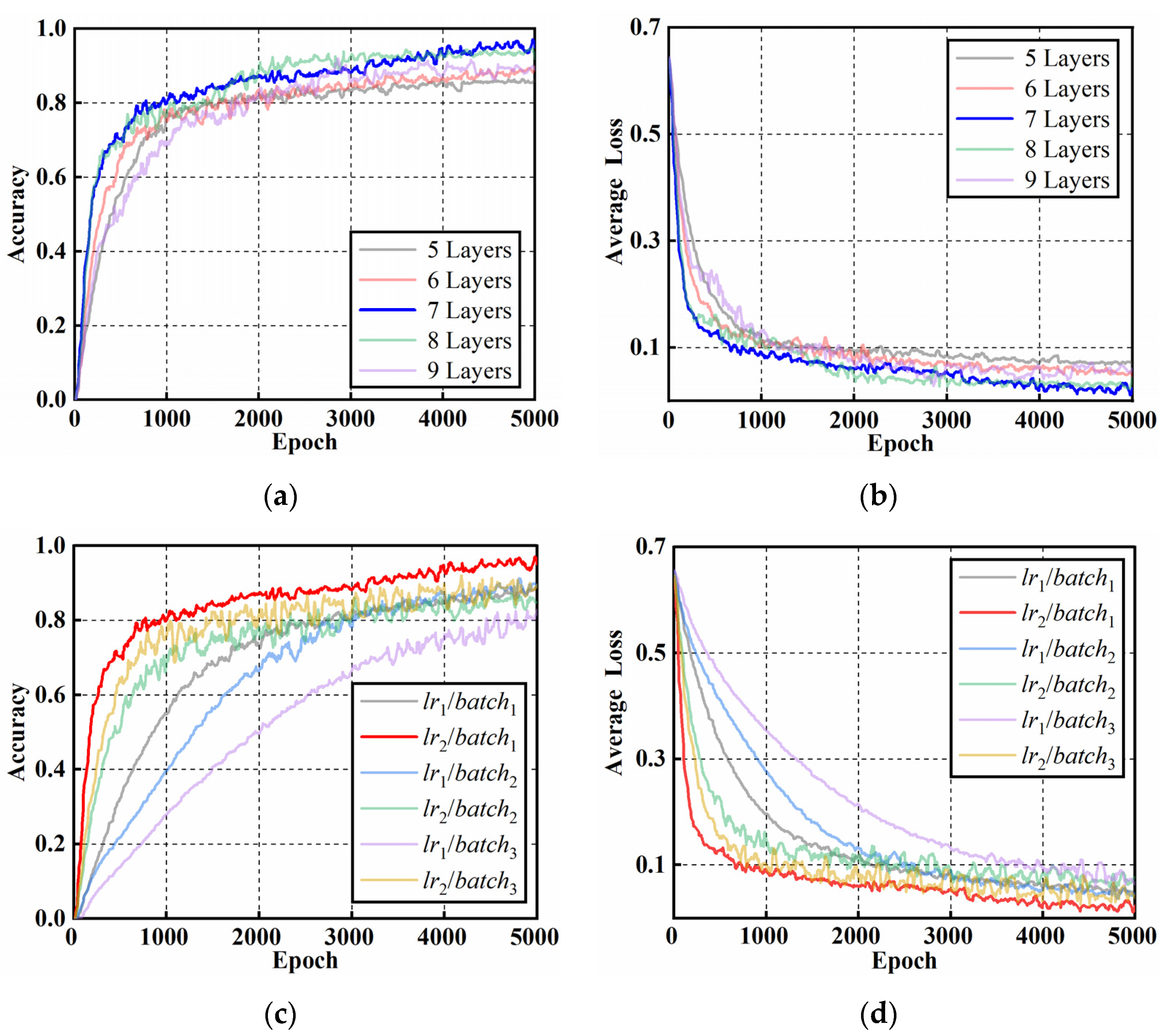
During the data generation process, three sets of data with varying substrate thicknesses have been generated. From the results, it can be observed that the inversion performance of the inversion model is similar for datasets with different substrate thicknesses. Therefore, we only provide an example using the dataset with a substrate thickness of 20 μm. Figure 5a,b illustrate how the accuracy and average loss change during training with the substrate thickness set to 20 μm and the number of convolutional layers varying from 5 to 9, with all other settings held constant. In the Figure 5, we emphasize the best-performing curve during the training process with a darker shade, represented by the solid blue line. From the Figure 5, it can be observed that as the training progresses, the predictive accuracy of the inversion model continuously improves, and the prediction error decreases, indicating that the inversion model is learning the mapping relationship between the scattering curves and the output structure. After 4000 epochs of training, both the accuracy and the average loss fluctuate around a certain level without significant changes, and the accuracy can eventually reach over 90%. This suggests that the inversion model has effectively learned the mapping relationship between the input and output. However, the differences among all solid lines in the graph are not particularly distinct, thus requiring a comprehensive assessment considering the performance of inversion models of different complexities on the test set and the time required to train the models. In Figure 6a, the blue line represents the performance of inversion models of different complexities on the test set, while the red line represents the time required to train models of different complexities. It can be observed from the blue line in the graph that the effectiveness of the model does not exhibit proportional improvement with increased structural complexity. When the model’s structure reaches a certain level, specifically with eight convolutional layers, its performance deteriorates, while the training time increases. The more complex the model, the longer the training time required, but the worse the inversion performance, which does not meet the selection criteria. Therefore, considering factors such as model complexity, performance, and training time, we selected the model with seven convolutional layers for subsequent experiments. Additionally, it is important to note that, in scenarios involving identical surface structures, the S-parameters corresponding to models with different substrate thicknesses show variability since substrate thickness is not a predictive parameter. Therefore, for datasets with different substrate thicknesses, it becomes imperative to train models with seven convolutional layers separately.
Figure 5c,d also illustrate the performance of the model on the training set with different combinations of hyperparameters, using the dataset with a substrate thickness of 20 μm as an example. The lr is set to 0.0001 or 0.0004, while the batch is set to 64, 128, or 256. The model structure remains the same. Similarly, we accentuated the curve representing the best performance during the training process, as indicated by the solid red line. Increasing the lr leads to amplified fluctuations in accuracy or average loss during the training process, consistent with theoretical expectations. Similarly, as the training process progresses, the predictive accuracy of the inversion models with different parameter combinations continues to increase, while the average loss keeps decreasing. After reaching a certain point, both metrics stabilize at a certain level without significant changes. Due to the relatively indistinct differences among the curves, we need to consider Figure 6b. In Figure 6b, similarly, the red and blue lines represent the time required for training and the performance on the test set, respectively. The time required for training is inversely proportional to the lr or batch size. The larger the batch or lr, the less time is needed for training, and vice versa. Based on these results, we prioritized the performance of inversion models on the test set as the primary criterion, followed by consideration of the training time (as the models trained with different parameter combinations show similar training times in the figure). Selecting an inversion model with good performance while requiring minimal additional computational resources is reasonable. In summarizing the existing model performance across different substrate thickness datasets, this work determined the optimal combination of parameters: lr and batch are set to 0.0004 and 64, respectively, for subsequent validation.
Based on the above analysis, whether it is models with different structural complexities or different parameter combinations, the optimal-performing models ultimately achieve a predictive accuracy of over 90%. This represents a significant improvement in accuracy compared to other metasurface design methods. It is worth noting that neither in the training nor testing processes did we perform any additional data preprocessing on the obtained simulation data, which further demonstrates the simplicity and efficiency of the method proposed in this work.

4.2. Inversion Verification

After confirming the appropriate lr and batch for the network architecture, we proceed to validate the inversion performance of the model. The overall process is as follows: for datasets with varying substrate thicknesses, three anticipated design objectives are input individually into the trained model, resulting in predicted 16-dimensional THz metasurface sensor surface structure matrices. Based on the element distribution within these matrices, EM simulation modeling is conducted, resulting in the corresponding S-parameters. Finally, a comparison is made between the expected values and the actual simulation results. The overall process is depicted in Figure 7.
In Figure 8, solid lines represent the expected S-parameter curves, while dashed lines depict the simulated results corresponding to the THz metasurface structures obtained from the inversion model predictions. Each expected S-parameter curve is selected arbitrarily from the test set. As observed from the graph, regardless of the substrate thickness (20 μm, 50 μm, or 80 μm), there is a close agreement between the solid and dashed lines, with significant overlap, indicating minimal error between the expected and actual values. This indirectly demonstrates the high accuracy and efficiency of the proposed inversion model. Furthermore, this process did not undergo any data preprocessing operations. During the data generation process, the substrate thickness has a significant impact on the electromagnetic characteristics of the metasurface model. However, based on the above results, the inversion model shows an excellent performance in predicting the S-parameter curves corresponding to metasurface models with different substrate thicknesses. This demonstrates that the thickness has almost no effect on the predictive performance of the inversion model. This proves the superiority of the inversion model designed in this study in terms of accuracy and provides an efficient design method for subsequent THz metasurface biosensors tailored to specific characteristics.

4.3. Prediction Time and Error

In this section, we quantitatively evaluate the time needed for the inversion method and the prediction error. We also record the time taken for each inversion prediction and the mean squared error (MSE) between predicted and simulated values, as depicted in Table 1. The formula for calculating the MSE is shown in Equation (5).
MSE = 1 n i = 1 n ( X i Y i ) 2
where Xi and Yi represent the expected and actual values, respectively, and n represents the total number of data points.
In the traditional design process of THz metasurface sensors, the influence of substrate thickness on performance is a factor that must be considered. However, as observed in the table, for models with different thicknesses, both the inversion time and the error between expected and simulated values are remarkably low. The method proposed in this work exhibits a nearly identical inversion performance for samples of different thicknesses, thereby demonstrating the efficiency of the proposed approach. Moreover, the method proposed in this work is compared with other methods, as depicted in Table 2. As Table 2 verifies, the proposed method not only proves suitable for THz metasurface sensor design but also exhibits the advantages of fast prediction and high precision without the need for additional optimization algorithms. The “√” in the table means that the heading method is used, and the “×” is not used. In contrast to conventional design methods, it excels in saving working time, conserving computing resources, reducing costs, and enhancing design efficiency, while also catering to a wider range of frequency bands. Therefore, this approach provides an efficient design method for THz metasurface sensors, which holds promising application prospects in the biomedical field.

5. Conclusions

This paper proposes the application of a deep learning model (one-dimensional convolutional neural network) for the rapid and efficient design of THz metasurface sensor surface structures. This method overcomes the drawbacks of traditional design approaches, such as time-consuming processes, high repetition, a strong reliance on specialized knowledge, and complex data preprocessing. Through a series of experimental results, including the performance of the inversion model for datasets with different substrate thicknesses, validation of the inversion model, and comparisons with other methods, it is evident that the proposed approach offers advantages such as high inversion accuracy, time efficiency, a low requirement for specialization, and simplicity of steps. The efficient inversion method is beneficial for the real-time prediction of THz metasurface sensor structures, enabling the real-time design of sensors in the biomedical field and accelerating subsequent biological analysis processes. However, the current work is limited by the simplicity of the inverted structures. In the future, we will represent the structure of THz metasurfaces in a more complex manner to better reflect real-world scenarios and demonstrate more unique electromagnetic properties.

Author Contributions

Conceptualization, D.J. and M.G.; software, D.J.; writing—original draft preparation, D.J.; writing—review and editing, G.Z.; supervision, B.W.; project administration, M.G.; funding acquisition, M.G. All authors have read and agreed to the published version of the manuscript.

Funding

This study was funded by the National Natural Science Foundation of China (62301611, 42174141); Shandong Provincial Natural Science Foundation (ZR2022QD082, ZR2021QF132, ZR2019MEE095); Fundamental Research Funds for the Central Universities (22CX06036A, 20CX05005A); Major Scientific and Technological Projects of CNPC (ZD2019-184-001); Youth Innovation Technology Project of Higher School in Shandong Province (2023KJ069).

Data Availability Statement

The data underlying the results presented in this paper are not publicly available at this time but may be obtained from the authors upon reasonable request.

Acknowledgments

We are deeply grateful to the reviewers and editors for their invaluable and constructive suggestions and comments that greatly improved the version of this article.

Conflicts of Interest

The authors declare no conflicts of interest.

References

  1. Fedorov, V.; Tzortzakis, S. Powerful Terahertz Waves from Long-wavelength Infrared Laser Filaments. Light Sci. Appl. 2020, 9, 186. [Google Scholar] [CrossRef] [PubMed]
  2. Ge, H.; Lv, M.; Lu, X.; Jiang, Y.; Wu, G.; Li, G.; Li, L.; Li, Z.; Zhang, Y. Applications of THz Spectral Imaging in the Detection of Agricultural Products. Photonics 2021, 8, 518. [Google Scholar] [CrossRef]
  3. Ge, Z.; Wang, Y.; Cao, Y.; Chen, H. Multilayer Flexible Metamaterials With Fano Resonances. IEEE Photonics J. 2016, 8, 4600109. [Google Scholar] [CrossRef]
  4. Gong, Y.; Quan, B.; Hu, F.; Zhang, L.; Jiang, M.; Lin, S. Intervalley Scattering Induced Terahertz Field Enhancement in Graphene Metasurface. Nano Lett. 2023, 23, 11051–11056. [Google Scholar] [CrossRef] [PubMed]
  5. Guan, M.; Sun, X.; Wei, J.; Jia, X.; Cheng, X.; Cheng, R. High-Sensitivity Terahertz Biosensor Based on Plasmon-Induced Transparency Metamaterials. Photonics 2023, 10, 1258. [Google Scholar] [CrossRef]
  6. Özer, Z.; Akdoğan, V.; Wang, L.; Karaaslan, M. Graphene-Based Tunable Metamaterial Absorber for Terahertz Sensing Applications. Plasmonics 2024. [Google Scholar] [CrossRef]
  7. Lu, Y.; Hale, L.L.; Zaman, A.M.; Addamane, S.J.; Brener, I.; Oleg, M.; Degl’Innocenti, R. Near-Field Spectroscopy of Individual Asymmetric Split-Ring Terahertz Resonators. ACS Photonics 2023, 10, 2832–2838. [Google Scholar] [CrossRef]
  8. Gupta, J.; Das, P.; Bhattacharjee, R.; Sikdar, D. Enhancing Signal-to-noise Ratio of Clinical 1.5T MRI Using Metasurface-inspired Flexible Wraps. Appl. Phys. 2023, 129, 725. [Google Scholar] [CrossRef]
  9. Cusano, A.M.; Quero, G.; Vaiano, P.; Cicatiello, P.; Principe, M.; Micco, A.; Ruvo, M.; Consales, M.; Cusano, A. Metasurface-assisted Lab-on-fiber Optrode for Highly Sensitive Detection of Vitamin D. Biosens. Bioelectron. 2023, 242, 115717. [Google Scholar] [CrossRef]
  10. Mishra, R.; Panwar, R.; Singh, D. Equivalent Circuit Model for the Design of Frequency-Selective, Terahertz-Band, Graphene-Based Metamaterial Absorbers. IEEE Magn. Lett. 2018, 9, 3707205. [Google Scholar] [CrossRef]
  11. Liu, X.; Sun, J.; Shi, Z.; Xiu, S.; Cui, Y.; Hou, Y.; Li, R.; Wang, N.; Zhang, L.; Li, X.; et al. Electric Field Dropping Effect Enhanced Extraordinary Sensitivity of THz Electromagnetically Induced Transparency Metamaterial. IEEE Sens. J. 2024, 24, 7807–7815. [Google Scholar] [CrossRef]
  12. Gaynutdinov, R.R.; Chermoshentsev, S.F. Metaelement Parameters Optimization for Creation Metamaterial with Given Electromagnetic Properties. In Proceedings of the 2021 International Russian Automation Conference (RusAutoCon), Sochi, Russia, 5 September 2021. [Google Scholar] [CrossRef]
  13. Qiu, T.; Shi, X.; Wang, J.; Li, Y.; Qu, S.; Cheng, Q.; Cui, T.; Sui, S. Deep Learning: A Rapid and Efficient Route to Automatic Metasurface Design. Adv. Sci. 2019, 6, 1900128. [Google Scholar] [CrossRef] [PubMed]
  14. Shi, X.; Qiu, T.; Wang, J.; Zhao, X.; Qu, S. Metasurface Inverse Design Using Machine Learning Approaches. J. Phys. D 2020, 53, 275105. [Google Scholar] [CrossRef]
  15. Pal, D.; Singhal, R.; Bandyopadhyay, A.K. Parametric Optimization of Complementary Split-Ring Resonator Dimensions for Planar Antenna Size Miniaturization. Wirel. Pers. Commun. 2022, 123, 1897–1911. [Google Scholar] [CrossRef]
  16. Haffa, S.; Hollmann, D.; Wiesbeck, W. The Finite Difference Method for S-Parameter Calculation of Arbitrary Three-Dimensional Structures. IEEE Trans. Microw. Theory Technol. 1992, 40, 1602–1610. [Google Scholar] [CrossRef]
  17. Yue, T.; Jiang, Z.; Panaretos, A.H.; Werner, D.H. A Compact Dual-Band Antenna Enabled by a Complementary Split-Ring Resonator-Loaded Metasurface. IEEE Trans. Antennas Propag. 2017, 65, 6878–6888. [Google Scholar] [CrossRef]
  18. Huang, X. Design of Miniaturized SIW Filter Loaded with Improved CSRR Structures. Electronics 2023, 12, 3789. [Google Scholar] [CrossRef]
  19. Xiong, J.; Ying, Z.; He, S. A Broadband Low Profile Patch Antenna of Compact Size with Three Resonances. IEEE Trans. Antennas Propag. 2009, 57, 1838–1843. [Google Scholar] [CrossRef]
  20. Carr, A.R.; Chan, Y.J.; Reuel, N.F. Contact-Free, Passive, Electromagnetic Resonant Sensors for Enclosed Biomedical Applications: A Perspective on Opportunities and Challenges. ACS Sens. 2023, 8, 943–955. [Google Scholar] [CrossRef]
  21. Zhang, M.; Guo, G.; Xu, Y.; Yao, Z.; Zhang, S.; Yan, Y.; Tian, Z. Exploring the Application of Multi-Resonant Bands Terahertz Metamaterials in the Field of Carbohydrate Films Sensing. Biosensors 2023, 13, 606. [Google Scholar] [CrossRef]
  22. Zaitsev, A.D.; Demchenko, P.S.; Kablukova, N.S.; Vozianova, A.V.; Khodzitsky, M.K. Frequency-Selective Surface Based on Negative-Group-Delay Bismuth–Mica Medium. Photonics 2023, 10, 501. [Google Scholar] [CrossRef]
  23. Barzegar-Parizi, S.; Vafapour, Z. Dynamically Switchable Sub-THz Absorber Using VO2 Metamaterial Suitable in Optoelectronic Applications. IEEE Trans. Plasma Sci. 2022, 50, 5038–5045. [Google Scholar] [CrossRef]
  24. Zhang, N.; Wu, W.; Zheng, G. Convergence of Gradient Method With Momentum for Two-Layer Feedforward Neural Networks. IEEE Trans. Neural Netw. 2006, 17, 522–525. [Google Scholar] [CrossRef] [PubMed]
  25. Ren, N.; Fu, Z.; Zhou, D.; Kong, D.; Liu, H.; Tian, S. Jitter Decomposition Meets Machine Learning: 1D-Convolutional Neural Network Approach. IEEE Commun. Lett. 2021, 25, 1911–1915. [Google Scholar] [CrossRef]
  26. Rawal, V.; Prajapati, P.; Darji, A. Hardware Implementation of 1D-CNN Architecture for ECG Arrhythmia Classification. Biomed. Signal Proces. 2023, 85, 104865. [Google Scholar] [CrossRef]
  27. Parhi, R.; Nowak, R.D. The Role of Neural Network Activation Functions. IEEE Signal Process. Lett. 2020, 27, 1779–1783. [Google Scholar] [CrossRef]
  28. Fu, S.; Wang, X.; Tang, J.; Lan, S.; Tian, Y. Generalized Robust Loss Functions for Machine Learning. Neural Netw. 2024, 171, 200–214. [Google Scholar] [CrossRef]
  29. Li, Y.; Ren, X.; Zhao, F.; Yang, S. A Zeroth-Order Adaptive Learning Rate Method to Reduce Cost of Hyperparameter Tuning for Deep Learning. Appl. Sci. 2021, 11, 10184. [Google Scholar] [CrossRef]
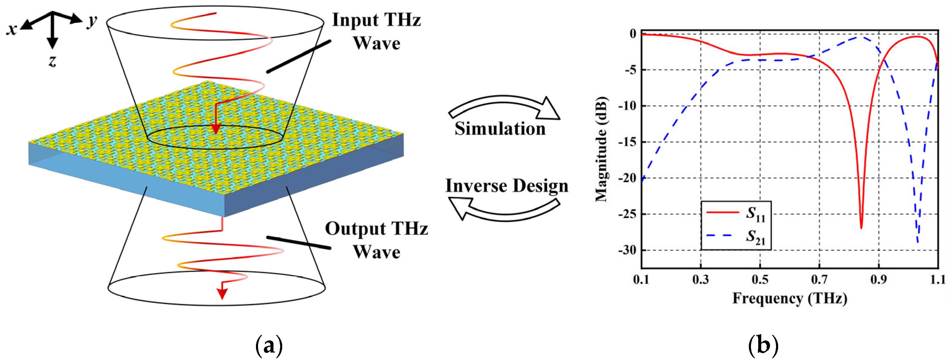
Figure 1. Schematic diagram of the THz metasurface sensor. (a) Interaction with THz waves; (b) S-parameter corresponding to metasurface sensors.
Photonics 11 00424 g001
Figure 2. One-dimensional convolution operation diagram.
Photonics 11 00424 g002
Figure 3. Binary-encoded unit structure diagram of THz metasurface sensor.
Photonics 11 00424 g003
Figure 4. Diagram of 1D CNN structure.
Photonics 11 00424 g004
Figure 5. Model training performance varies with different model complexities and different hyperparameter combinations, with a substrate thickness of 20 μm. (a,b) Different convolution layers; (c,d) different combinations of lr and batch. lr1 and lr2 are 0.001 and 0.0004, respectively; batch1, batch2, and batch3 are 64, 128, and 256, respectively.
Photonics 11 00424 g005
Figure 6. Model performance varies across datasets with different model complexities and hyperparameter combinations. (a) Different convolution layers; (b) different combinations of lr and batch.
Photonics 11 00424 g006
Figure 7. Diagram of the prediction process.
Photonics 11 00424 g007
Figure 8. Comparison between prediction (Pred.) and simulation (Sim.) S-parameters of metasurface structures with different substrate thicknesses: (a) h = 20 μm; (b) h = 50 μm; (c) h = 80 μm.
Photonics 11 00424 g008
Table 1. The time required for predicting inversion and the mean squared error.
Number of Example123
Prediction timeh = 20 μm0.014s0.014s0.014s
h = 50 μm0.065s0.060s0.013s
h = 80 μm0.014s0.057s0.015s
Prediction Error (MSE)h = 20 μm0.0090.0010.002
h = 50 μm0.4380.4530.086
h = 80 μm0.3010.0170.001
Table 2. Comparison of the proposed method with other methods.
Method NamePrediction AccuracyData PreprocessingEncoding and Decoding MeansApplication Band
This method93.3%××0.1–1.1 THz
AMID81.6%3–20 GHz
REACTIVE76.5%2–20 GHz
Disclaimer/Publisher’s Note: The statements, opinions and data contained in all publications are solely those of the individual author(s) and contributor(s) and not of MDPI and/or the editor(s). MDPI and/or the editor(s) disclaim responsibility for any injury to people or property resulting from any ideas, methods, instructions or products referred to in the content.