Intermodal Fiber Interferometer with Spectral Interrogation and Fourier Analysis of Output Signals for Sensor Application

Abstract

Interferometric fiber-optic sensors provide very high measurement accuracy and come with many other benefits. As such, the study of signal processing techniques for fiber-optic interferometers in order to extract information about external perturbation is an important area of research. In this work, the method of Fourier analysis was applied to extract information from the output signals of an intermodal fiber interferometer with spectral interrogation. It is shown that the external perturbation can be measured by obtaining the phase spectrum of the spectral transfer function of an intermodal fiber interferometer and determining the phase difference of a certain pair of mode groups. A mathematical model of this approach was developed, taking into account the parameters of the laser and the optical fiber, the number of excited mode groups, and the parameters of external perturbation. The theoretically considered method of Fourier analysis was experimentally verified, and it was proved to provide a linear response to external perturbation in a wide dynamic range.

1. Introduction

Interferometric fiber-optic sensors of physical quantities have been actively used in science and technology over the past few decades [1,2,3,4,5,6,7,8,9,10]. The reason for this is the combination of very high achievable measurement accuracy and a number of other advantages—electromagnetic neutrality, biological compatibility, and small size and weight. All this stimulates the increased interest in the study of this type of sensors.

One of the types of such sensors is based on an intermodal fiber interferometer (IFI). Simplicity and relatively low cost, which are the main advantages of IFIs, support the interest in the investigation of IFI-based sensors for medical applications, temperature, pressure, strain, vibration sensing, and other applications [11,12,13,14,15,16,17,18,19,20,21,22]. Such applications of IFIs as the implementation of IFI-based sensors with polymer optical fiber [23,24,25,26,27] and the use of IFI-based sensors for multiparametric measurements [28,29,30] are also actively being investigated.

The basic principle of IFI operation is as follows. A multimode fiber (MMF) acts as the sensitive element, in which a coherent light source excites a certain number of modes. If an external perturbation affects the MMF, the relative phase differences of the modes change, and this, in turn, leads to a change in the configuration of the interference pattern (speckle pattern) at the output end of the MMF. Insofar as the output signal is being diaphragmed, changes in the output light intensity are observed, which are actually the IFI signal. Due to the fact that the IFI signal contains information about the magnitude of the perturbation on the IFI, it can be used to measure this perturbation.

There are two problems that seriously complicate the feasibility of using IFIs to implement sensors, namely the nonlinearity of the IFI signal and its susceptibility to signal fading, that is, unpredictable variations in the IFI signal amplitude and its contrast with changes in environmental conditions. There are several ways to eliminate these obstacles: these are methods of adaptive registration of IFI signals [31], methods of averaging its signals [32,33,34,35,36], and correlation analysis methods for speckle patterns at the MMF output [37,38,39,40,41,42,43]. These methods can significantly reduce the signal fading, but they do not solve the problem of its nonlinearity.

Recently, methods related to spectral interrogation of fiber-optic sensors have been actively developed [44,45,46,47,48,49,50]. These approaches are actively used in the implementation of sensors based on single-mode–multimode–single-mode (SMS) structures [30,51,52,53,54,55].

The spectral interrogation approach can also be used for an IFI. In this article, we refer to this IFI implementation as an intermodal fiber interferometer with spectral interrogation (IFISI).

The authors of this paper previously considered the approach of correlation analysis of IFISI signals [56,57] and proved that this approach really provides a linear and stable response to external perturbation. Nevertheless, its main disadvantage was revealed, namely its relatively small dynamic range, within which a linear response to external perturbation can be obtained.

In this paper, an approach based on Fourier analysis of IFISI signals is considered. This approach is based on obtaining the phase spectrum of the IFISI spectral transfer function and determining the phase difference of a certain pair of mode groups. The determined phase difference of a pair of mode groups linearly depends on the external perturbation on the MMF, which makes it possible to use this approach in the implementation of sensors of physical quantities.

It is important to note that this approach is actively used in the implementation of sensors based on SMS structures [30,51,52,53]. However, these SMS structures utilize a relatively short step-index MMF segment. In our work, we applied this method to the IFISI with long graded-index MMF. Moreover, most of the published works on SMS sensors treat spectral interrogation rather empirically, omitting proper theoretical analysis of mode propagation.

As a result of our research, a mathematical model of the IFISI with Fourier analysis of its signals was developed. This model takes into account all the main parameters of the IFISI—the parameters of the MMF, the number of excited mode groups, and the performance characteristics of the laser. Using this model, numerical simulation of an IFISI with Fourier analysis of its signals was carried out. The Fourier analysis of the IFISI signal approach was implemented and investigated experimentally. The experimental results are consistent with the results of calculations based on the developed mathematical model.

Our research demonstrates that the Fourier analysis of IFISI signals provides a linear response to external perturbation. Thus, this approach can be used in the implementation of a physical quantity sensor based on an IFISI with a long MMF.

2. Theory

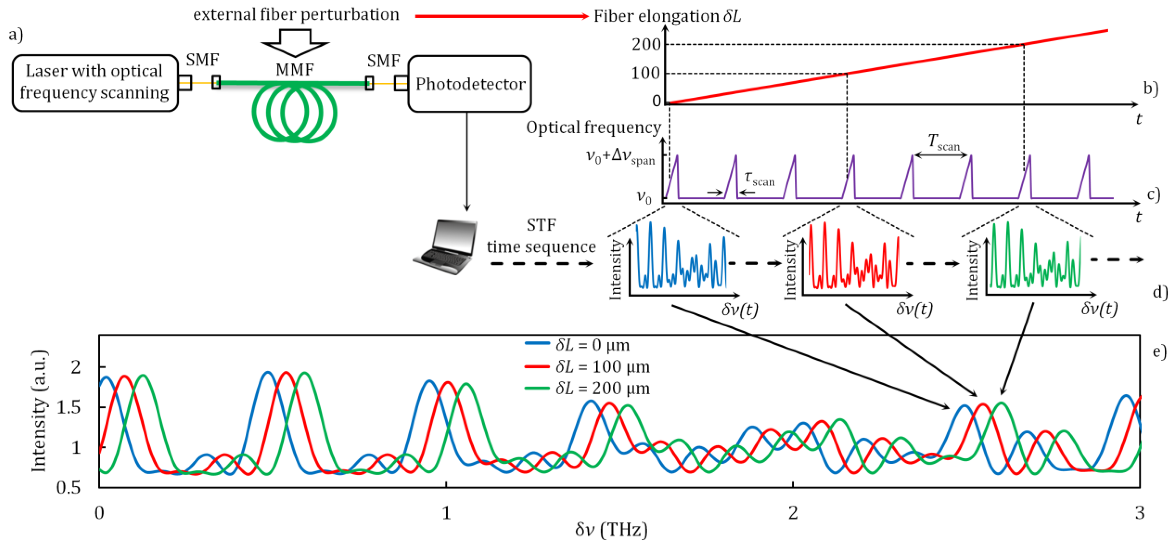
2.1. Principal Scheme and Basic Principles of Operation

Figure 1 illustrates the basic operating principles of the IFISI. The schematic design of such an IFISI is shown in Figure 1a. The laser emits light, the optical frequency of which is scanned in a certain range [v₀; v₀ + Δν_span]. The duration of one scan is τ_scan; the period of the scans is T_scan.

The light is launched into the MMF, which acts as a sensitive element to external perturbation. After passing through the MMF, the light is spatially filtered (for example, by connecting the output end of the MMF with the single-mode fiber (SMF), whose core diameter is smaller) and then received by a photodetector.

The external fiber perturbation (EFP) leading to a change in the MMF length is considered. In Figure 1, an EFP is presented, leading to a linear elongation of the MMF δL (Figure 1b).

As a result of each optical frequency scan, the dependence of the IFISI signal on the optical frequency is formed on the photodetector. This dependence appears to be the spectral transfer function (STF). Figure 1c shows a sequence of optical frequency scans, and Figure 1d shows three STFs at an enlarged scale on a time axis.

As EFP affects the IFISI, the STF is modified; namely, it is shifted along the optical frequency scale. This is clearly seen in Figure 1e, where the three STFs obtained at different magnitudes of the MMF elongation δL are shown in one plot.

Thus, it is obvious that the EFP can be measured by analyzing the STF change. In the following sections, it will be shown that Fourier analysis of the STF approach can be used to reach this goal.

It is important to note that in order to apply this approach to measuring the EFP, several conditions must be met, as follows:

• The duration of one optical frequency scan τ_scan should be small enough that, over the time interval of the τ_scan, the value of MMF elongation δL can be considered constant;
• The period of the scan sequence T_scan should be significantly shorter than the characteristic period of EFP (in accordance with the Nyquist criterion).

Within the framework of our analysis, we knowingly assume that these conditions are met.

2.2. Basic Expressions and Physical Interpretation of STF

Before starting a theoretical analysis, it is necessary to make a number of important assumptions. We assume that the laser output intensity does not depend on the optical frequency. The number of excited mode groups and their amplitudes also do not depend on the optical frequency. It should be noted that, strictly speaking, the number of mode groups increases with increasing optical frequency. However, in the scanning range under consideration, the difference in the number of mode groups does not exceed one, so this effect can be neglected. The MMF itself is isotropic and lossless. We confine our consideration to external perturbations that do not give rise to mode coupling in the MMF, so this effect can also be neglected. All these assumptions make it possible to significantly simplify analytical expressions without significantly reducing their accuracy.

The input data for the calculations (MMF parameters and laser parameters), the results of which are given in this section, were chosen to be the same as they were when carrying out the experiments. These parameters are shown in

Table 1. Laser and MMF parameters used in calculations.

Optical frequency ν0 (THz)	193.41
Laser linewidth Δνa (GHz)	0.5
Fiber core radius a (µm)	25
Refractive index at the core axis n	1.48
Relative difference of refractive indices Δ	0.01
Profile parameter α	2.065
Material dispersion parameter δ	0.001
MMF length L (m)	40

.

It is notable that the refractive index profile parameter α was not given by the manufacturer of the optical fiber used in the experiments. However, insofar as the α parameter controls the delay time between different mode groups [58], its value can be deduced from the preliminary measurements of the delay times between the mode groups in the MMF used. An explanation of this method of α parameter estimation is given at the end of this section. Thus, obtained value of α is also shown in Table 1.

The parameter variables in the calculations (the number of excited mode groups, and the scanning range of the optical frequency Δν_span) are not presented in Table 1.

An expression describing the IFISI signal at some point on the MMF output end, depending on the magnitude of the EFP (MMF elongation δL) and the optical frequency ν, is written as follows [33].

$$I(\nu )=\frac{1}{M}{\displaystyle \sum _{k=1}^M{\left(a_k\right)}^2+}\frac{2}{M^2-M}{\displaystyle \sum _{i=2}^M{\displaystyle \sum _{k=1}^{i-1}{a}_k{a}_i\cos \left[\Delta {\beta }_{\mathrm{ki}}(\nu )(L+\mathsf{\delta }L)+\left({\phi }_k-{\phi }_i\right)\right]}}$$

(1)

where the first term is the constant component of the light intensity, the second term is the interference component, M is the number of excited mode groups, L is the MMF length, δL is the magnitude of MMF elongation as a result of EFP, ν is the optical frequency of the light source, Δβ_ki is the difference between the propagation constants of the k-th and i-th mode groups at the frequency ν [58], a_i is the amplitude of the i-th mode group, and φ_i is a random phase shift of the i-th mode group occurring on local inhomogeneities of the MMF.

By expanding Δβ_ki into a Taylor series in the vicinity of the optical frequency ν₀ and introducing a multiplier characterizing the effect of the laser linewidth, Equation (1) can be written [57]:

$$\begin{array}{l}I(\mathsf{\delta }\nu )=\frac{1}{M}{\displaystyle \sum _{k=1}^M{\left(a_k\right)}^2+}\frac{2}{M^2-M}{\displaystyle \sum _{i=2}^M{\displaystyle \sum _{k=1}^{i-1}{a}_k{a}_i\frac{\sin (\pi \cdot \Delta t_{\mathrm{ki}}\cdot \Delta {\nu }_a)}{\pi \cdot \Delta t_{\mathrm{ki}}\cdot \Delta {\nu }_a}\cdot }}\cos \left[\Delta {\beta }_{\mathrm{ki}}({\nu }_0)(L+\mathsf{\delta }L)+2\pi \Delta t_{\mathrm{ki}}\mathsf{\delta }\nu +\left({\phi }_k-{\phi }_i\right)\right]\end{array}$$

(2)

where ν₀ is the optical frequency of the light source, δν is the value of the optical frequency detuning from ν₀, Δν_a is the laser linewidth, and Δt_ki is the difference in propagation times of the k-th and i-th mode groups (delay time between the mode groups), determined [58] in accordance with Equation (3).

$$t_k=\frac{nL}{c}\left[1+\frac{\alpha -2-4\delta }{\alpha +2}\Delta {\left(\frac{k}{N}\right)}^{\frac{2\alpha }{\alpha +2}}+\frac{3\alpha -2-8\delta }{\alpha +2}\frac{{\Delta }^2}{2}{\left(\frac{k}{N}\right)}^{\frac{4\alpha }{\alpha +2}} \right]$$

(3)

where k is the mode group index, n is the refractive index at the core axis, c is the speed of light, α is the refractive index profile parameter, Δ is the relative difference in refractive indices, N is the maximum number of mode groups for a given MMF, and δ is the material dispersion parameter [58].

In fact, the STF is expressed by Equation (2). Figure 2a–c show three STFs calculated for a different number of mode groups M.

The STF obtained by scanning the optical frequency for the case of two excited mode groups (Figure 2c) has a harmonic shape. The physical interpretation of this is quite simple: Two mode groups can be considered as two interfering beams passing through different optical paths. With a linear change in the optical frequency, the phase difference of these mode groups changes linearly, so the corresponding IFISI signal is harmonic. At the same time, as noted earlier, the EFP on the MMF also causes a change in the phase difference of the mode groups excited in the MMF. Consequently, the EFP on the MMF leads to a shift of the STF along the frequency scale (the red dotted line in Figure 2c).

The STFs shown in Figure 2a,b have more complex shapes. This is explained by the fact that these STFs are a superposition of harmonic signals, each of which characterizes the interference of a pair of mode groups with certain amplitudes and phases.

Since the STF is generally a superposition of harmonic signals, the Fourier transform can be applied to the STF. The result of this transform is a set of complex spectral components, each of which corresponds to a separate pair of mode groups.

In this case, the modulus of a certain spectral component is associated with the corresponding mode groups’ amplitudes and the argument with the mode groups’ phase difference. Since the EFP (MMF elongation δL) leads to a change in the phase difference of the mode groups, it is obvious that the EFP can be measured by determining the phase difference of a pair of mode groups, which is uniquely related to the argument of the corresponding spectral component of the Fourier image.

By applying the complex Fourier transform to Equation (2), using well-known mathematical relations [59], it is possible to obtain the expression for the Fourier image of the STF:

$$S(\Delta t)=\frac{2}{M^2-M}{\displaystyle \sum _{i=2}^M{\displaystyle \sum _{k=1}^{i-1}{a}_k{a}_i}}\cdot \frac{\sin (\pi \cdot \Delta t_{\mathrm{ki}}\cdot \Delta {\nu }_a)}{\pi \cdot \Delta t_{\mathrm{ki}}\cdot \Delta {\nu }_a}\cdot \frac{\sin \left[\pi \cdot \Delta {\nu }_{span}\cdot \left(\Delta t_{\mathrm{ki}}-\Delta t\right)\right]}{\pi \cdot \Delta {\nu }_{span}\cdot \left(\Delta t_{\mathrm{ki}}-\Delta t\right)}\cdot \exp \left[i\left(\Delta {\beta }_{\mathrm{ki}}({\nu }_0)\left(L+\mathsf{\delta }L\right)+\Delta {\phi }_{ki}\right)\right]$$

(4)

where Δt is the time parameter characterizing the delay between the mode groups, and Δν_span is the optical frequency scanning range.

Figure 2d–f show the results of calculating the moduli of the Fourier images of the STF, presented in Figure 2a–c.

It can be seen from Figure 2d–f that the presented spectral characteristics correspond to the actual composition of the mode groups excited in the MMF. The variable Δt, traced along the abscissa axis, actually characterizes the delay time between the mode groups. The delay time between the mode groups Δt_ki and, consequently, the type of the corresponding spectrogram depend on the MMF parameters, such as the MMF length, the refractive index profile parameter α, the numerical aperture, etc.

Summarizing the above consideration, the EFP can be measured through the following steps:

• Register the sequence of STF changes produced by the EFP;
• Perform the Fourier transform of each STF; select the spectral component Δt_ki corresponding to some pair of mode groups, and for this spectral component find the value of the argument;
• Determine the magnitude of the EFP by observing the change in the argument of the corresponding spectral component.

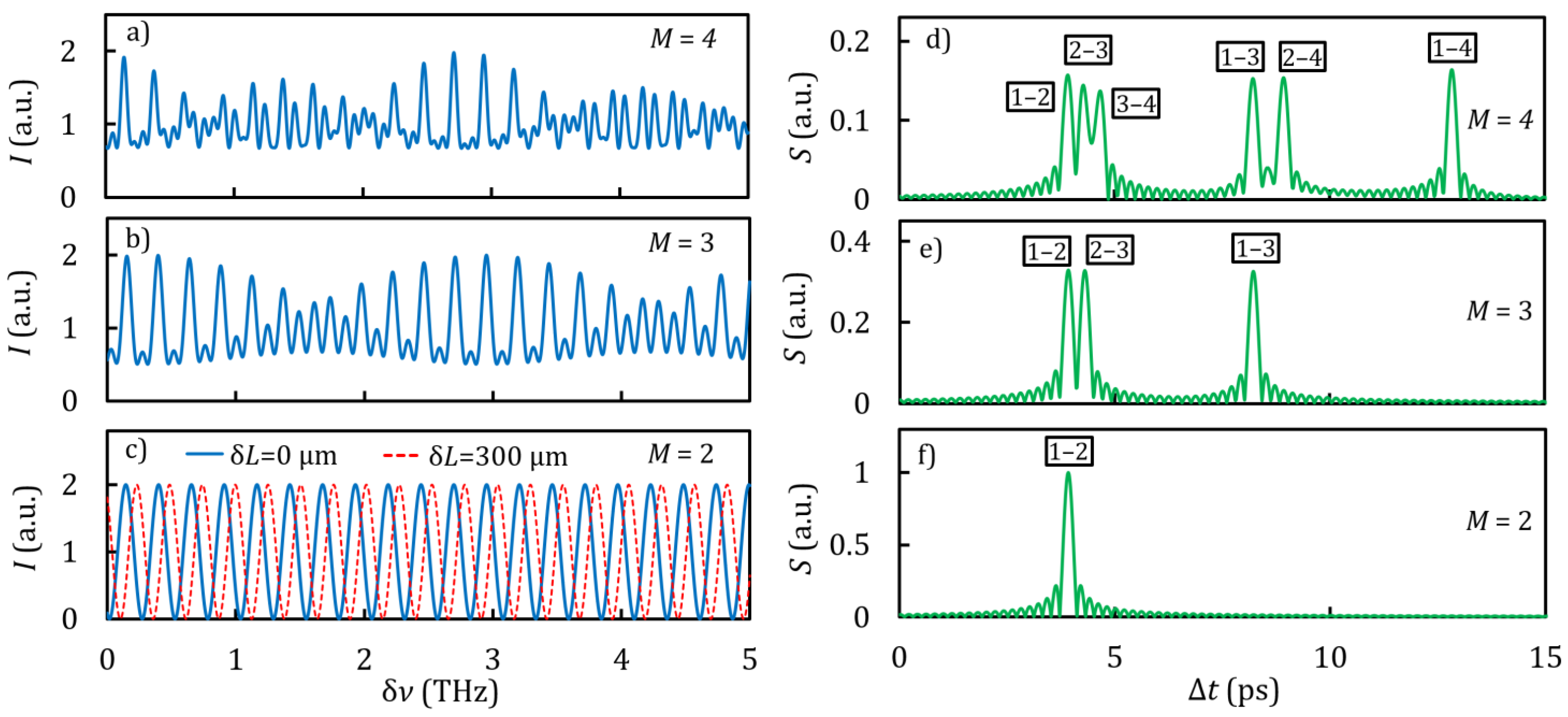
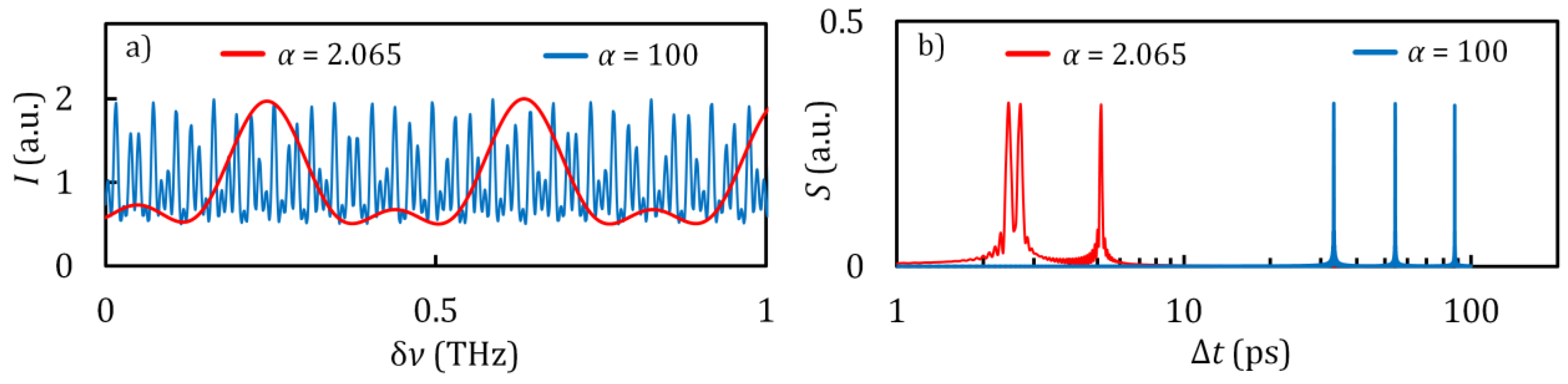
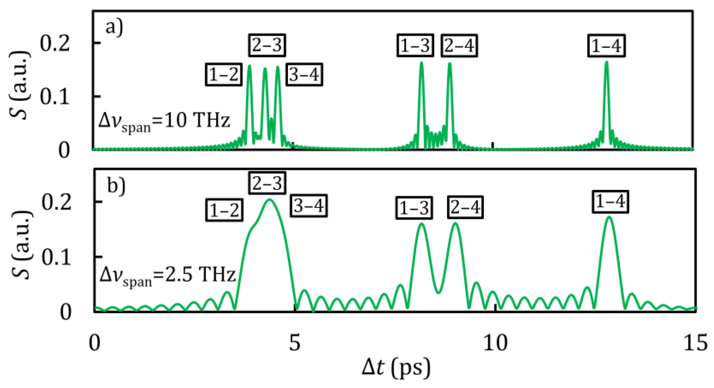
2.3. Numerical Simulation of the IFI with Spectral Interrogation and Fourier Analysis of Its Signals

As can be seen from Equation (4), the Fourier image of the STF and, consequently, the IFISI response to EFP depend on all the main IFISI parameters. Meanwhile, different parameters have different influences on the IFISI operation. This section discusses the impact of the most important of these parameters.

One of the most important parameters is the delay time between the mode groups Δt_ki. As can be seen from Equation (3), Δt_ki depends on the most important IFISI parameters, in particular on the MMF length L and the profile of the refractive index taken into account in Equation (3) through the parameter α.

Figure 3 shows the STFs and the moduli of their Fourier images calculated in accordance with Equations (2) and (4) for step-index and graded-index MMF.

It can be seen from Figure 3a that in the case of step-index MMF, the STF contains significantly more periods than the STF for the case of graded-index MMF. This is due to the fact that the delay time between mode groups in step-index MMF is significantly longer than in graded-index MMF.

To implement the approach of Fourier analysis of IFISI signals, it is necessary to select the refractive index profile, the MMF length, and the optical frequency scanning range Δν_span in such a way that the STF contains several periods, since this is a condition for obtaining a Fourier image corresponding to the composition of excited mode groups.

Another important parameter is the laser linewidth Δν_a. Calculations using Equation (4) showed that the amplitudes of the spectral components in the Fourier image of the STF depend on the value of Δν_a (Figure 4).

Figure 4 shows that the amplitude of the spectral component depends on Δν_a as a function of |sin(x)/x|, and the position of the zeros is determined by the ratio Δν_a = m/Δt_ki, where m = 1, 2, …. This is explained by the fact that each point of the STF, in fact, is the result of integrating the light intensity in the frequency range Δν_a. Thus, when this ratio is fulfilled, the integration interval is equal to or an integer number of times greater than the period of the harmonic component of the STF corresponding to this pair of mode groups, which leads to the disappearance of this harmonic component from the spectrum.

It is important to note that there is another physical interpretation of the results presented in Figure 4. A decrease in the spectral component magnitude with an increase in the laser linewidth Δν_a is associated with a decrease in the coherence of the IFISI’s operating mode. Indeed, for constructive interference of two beams, it is necessary that the coherence length of the laser is much greater than the path difference between these beams. As noted earlier, mode groups act as interfering beams in the IFISI. An increase in the laser linewidth Δν_a could be interpreted as a decrease in coherence length. Thus, when the coherence length of the laser approaches the path difference of a pair of mode groups, the magnitude of the corresponding spectral component starts to decrease. The first zero occurs when the coherence length equals the path difference of that pair of mode groups.

Another important parameter is the optical frequency scanning range Δν_span. Obviously, its value conditions the number of periods of the STF and thus the resolution of the delay time Δt between the mode groups in the Fourier image.

Figure 5 shows the moduli of the Fourier images of the STF calculated at different values of Δν_span. It can be seen that with an insufficient value of Δν_span, the resolution deteriorates, which leads to the failure in resolution of close spectral components.

However, choosing a too large optical frequency scanning range Δν_span also has some disadvantages.

First, in our analysis, we deliberately assume that the output intensity of the laser, as well as the number of mode groups and their amplitudes, do not depend on the optical frequency. If the optical frequency scanning range is too large, these conditions may be violated. This situation has the following effect on the STF and the corresponding Fourier image. As noted earlier, the STF is a superposition of harmonic signals, each of which corresponds to a specific pair of mode groups. Obviously, the dependence of the laser output intensity and the number of mode groups and their amplitudes on the optical frequency leads to the fact that harmonic signals corresponding to pairs of mode groups are amplitude-modulated. This, in turn, leads to the appearance of additional spectral components in the Fourier image of the STF.

Secondly, in our theoretical analysis, we expand the propagation constants in the vicinity of a central frequency and confine ourselves to the linear term only. However, due to the presence of material dispersion in the MMF, the nonlinear terms may contribute markedly to the propagation constants. This leads to the fact that harmonic signals corresponding to pairs of mode groups are frequency-modulated. This also leads to the appearance of additional spectral components in the Fourier image.

The presence of additional spectral components in the Fourier image of the STF entails the following difficulties. Firstly, it complicates the interpretation of the Fourier image in terms of determining the correspondence between spectral components and corresponding pairs of modes. Secondly, a situation may occur where additional spectral components are superimposed on a spectral component corresponding to a pair of mode groups. This situation can lead to a nonlinearity of the IFISI response.

Thus, the choice of the optimal value of the optical frequency scanning range should be made taking into account all the above factors.

As mentioned above, the principle of the approach of Fourier analysis of IFISI signals is based on determining the argument of the spectral component corresponding to a certain pair of mode groups. It can be seen from Equation (4) that the Fourier image of the STF is the sum of complex terms in exponential form; therefore, finding the argument explicitly is a non-trivial task.

However, since Equation (4) contains the multipliers sin[π∙Δν_span∙(Δt_ki − Δt)]/[π∙Δν_span∙(Δt_ki − Δt)], it is obvious that for cases Δt = Δt_ki (that is, for spectral components corresponding to pairs of mode groups) Equation (4) can be brought to the form

$$S({\left.\Delta t\right|}_{\Delta t=\Delta t_{\mathrm{ki}}})=\frac{2}{M^2-M}\cdot a_k{a}_i\cdot \exp \left[i\left(\Delta {\beta }_{\mathrm{ki}}({\nu }_0)\left(L+\mathsf{\delta }L\right)+\Delta {\phi }_{\mathrm{ki}}\right)\right]$$

(5)

From Equation (5), the argument can be easily expressed as

$$\Phi ({\left.\Delta t\right|}_{\Delta t=\Delta t_{\mathrm{ki}}})=\Delta {\beta }_{\mathrm{ki}}({\nu }_0)\mathsf{\delta }L+\Delta {\beta }_{\mathrm{ki}}({\nu }_0)L+\Delta {\phi }_{\mathrm{ki}}$$

(6)

where the first term corresponds to a change in the phase difference between the k-th and i-th mode groups as a result of EFP, the second term corresponds to a constant phase shift over the MMF length, and the third term is a random phase shift occurring on local inhomogeneities of the MMF.

It can be seen from Equation (6) that the argument linearly depends on the EFP magnitude. In this case, the steepness of the dependence is determined by the difference in the propagation constants Δβ_ki of the selected pair of mode groups. Figure 6 shows the dependence of the value of the Fourier image argument of the STF on the EFP magnitude for six pairs of mode groups.

It can be seen from Figure 6 that with an increase in the index difference in a pair of mode groups, the steepness of the characteristic increases. Accordingly, the steepness of the IFISI response to EFP depends on the selected pair of mode groups.

At the same time, for pairs of mode groups whose index differences are the same, the steepness is almost identical. This is due to the fact that in graded-index MMF, the dependence of the propagation constant value of the mode group on its index is close to linear [58].

It is important to note that the developed mathematical model makes it possible to determine such parameters of an IFISI as the number of excited mode groups, their relative amplitudes, and the delay times between the mode groups. This can be performed by comparing the experimentally obtained STF with the STF calculated in accordance with Equation (4). It was this approach that was applied to estimate the value of the refractive index profile parameter α of MMF used in the experiment.

Finally, this section presents a mathematical model describing the IFISI with Fourier analysis of its signals. It is shown that the proposed mathematical model makes it possible to analyze the IFISI, taking into account all its main parameters, such as the MMF parameters, optical frequency scanning parameters, and number of excited mode groups.

As a result of the calculations performed, it is shown that the mode group phase differences linearly depend on the EFP magnitude δL. Thus, based on this, it can be concluded that it is possible to obtain a linear response to EFP by applying the approach of determining the Fourier image argument of the STF of the IFISI.

3. Experimental Procedure

A measuring circuit based on the IFISI with Fourier analysis of its signals was implemented experimentally. This section presents the experimental results and their comparison with the results of calculations based on the mathematical model presented in the previous section.

3.1. Experimental Setup

The scheme of the experimental setup is shown in Figure 7.

A four-channel FBG NI PXIe 4844 interrogator (1) was used as a scanning light source and photodetector. The optical frequency was scanned according to the sawtooth law, and the scanning parameters are as follows: the scanning wavelength range is 20 nm (1550–1570 nm), which corresponds to the optical frequency band 2.5 THz, the scanning wavelength step is δλ = 4 pm (0.5 GHz), the scanning frequency is 10 cycles per second, the duration of one scan is τ_scan = 2.5 ms, and the optical power is 0.06 mW.

The choice of the optical frequency scanning range Δν_span is based on the considerations set out in Section 2.3. On the one hand, the value of Δν_span should be sufficient so that the STF contains a sufficient number of periods, which is a condition for obtaining a correct Fourier image. On the other hand, the choice of an excessive value of Δν_span may lead to the appearance of additional spectral components in the Fourier image (the reasons for the appearance of additional spectral components are discussed in detail in Section 2.3). As a result of our measurements, we found the compromise value for the optical frequency scanning range in our experimental setup to be Δν_span = 2.5 THz.

To isolate the input and output optical radiation, an optical circulator was installed in the circuit (2). Light was introduced into the MMF (Graded Index Corning 50/125 MMF with NA = 0.2 and length L = 40 m) (3) through an FC/PC connector (2). After passing the MMF, the light was spatially filtered by connecting the output end of the MMF and SMF using the FC/PC connector (5).

The main part of the MMF was wound on a cylindrical piezoceramic modulator with a diameter of 5 cm, used in the experimental scheme to implement an EFP on the MMF (MMF elongation according to the harmonic law with a frequency of 0.5 Hz and a magnitude from 0.1 to 220 μm). The EFP was obtained by applying a harmonic voltage with a specified amplitude to the modulator. In order to determine the dependence of the EFP magnitude on the voltage applied to the modulator, we calibrated the modulator using a Mach–Zehnder interferometer.

The choice of the frequency of EFP was made based on the following considerations. As mentioned earlier, the frequency of EFP should be less than the scanning frequency in accordance with the Nyquist criterion. Since the sampling frequency of the interrogator is 10 scans per second, we chose an EFP frequency of 0.5 Hz, which provides 20 scans for one period of EFP.

3.2. Experimental Results and Discussion

Figure 8 plots the experimental STF and the corresponding modulus of the Fourier image. Figure 8b also plots the modulus of the Fourier image calculated using Equation (4). The number of mode groups M and their amplitudes a_k were selected based on the number of spectral components in the experimental Fourier image and their amplitudes, respectively. The remaining calculation parameters are known for the MMF used and are listed in Table 1.

The experimentally obtained modulus of the Fourier image is consistent with the modulus of the Fourier image calculated by Equation (4). It is seen that 4 mode groups are excited in the MMF.

It can be seen from Figure 8b that the scanning range Δν_span = 2.5 THz is insufficient to resolve the spectral components corresponding to the pairs of mode groups 1–2, 2–3, and 3–4; therefore, one spectral component with Δt = 4 ps corresponds to these pairs of mode groups.

Figure 9 shows the dependence of the magnitude of the spectral components on the laser linewidth Δν_a. It can be seen that the results of the experiment are consistent with the results of the calculation using Equation (4).

The following are the results of measuring the EFP by Fourier analysis of IFISI signals. The sequence of steps was as follows:

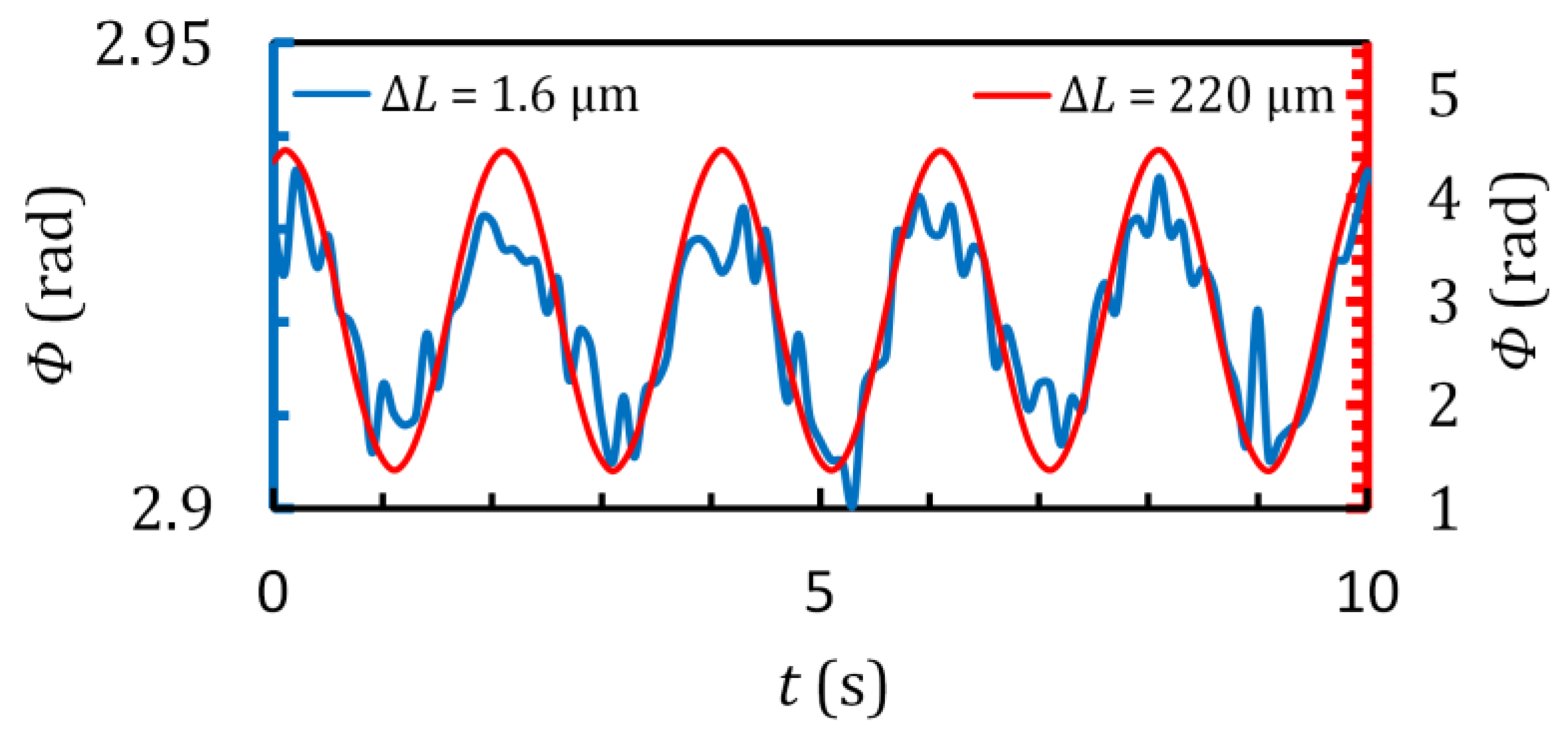
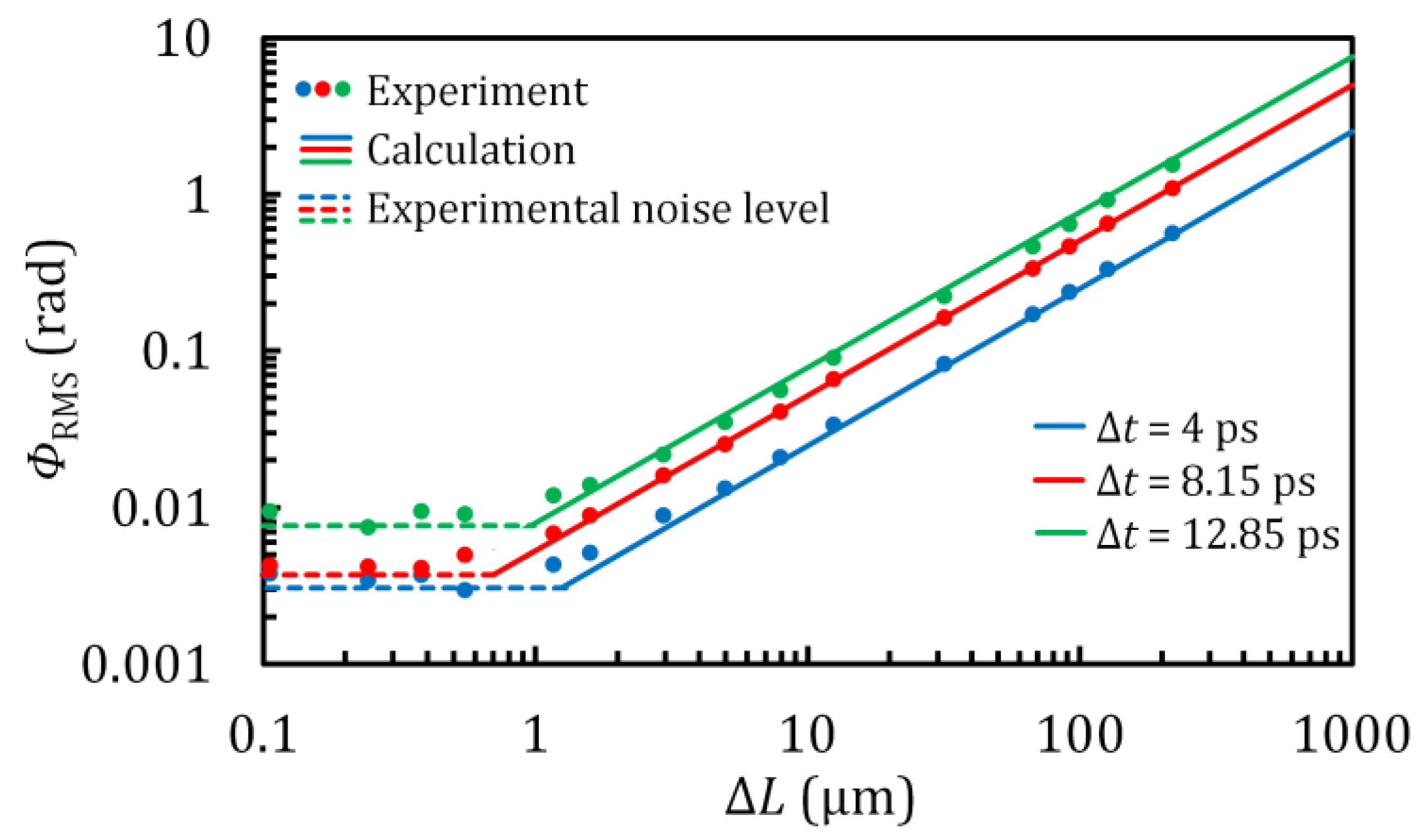
• Using a piezoceramic modulator, the MMF length was modulated according to the harmonic law (modulation frequency 0.5 Hz, magnitude from 0.1 to 220 μm).
• Sets of 10 STFs per second were recorded using the interrogator. A fast Fourier transform (FFT) was performed on each STF in real time, the result of which was the Fourier image of the STF.
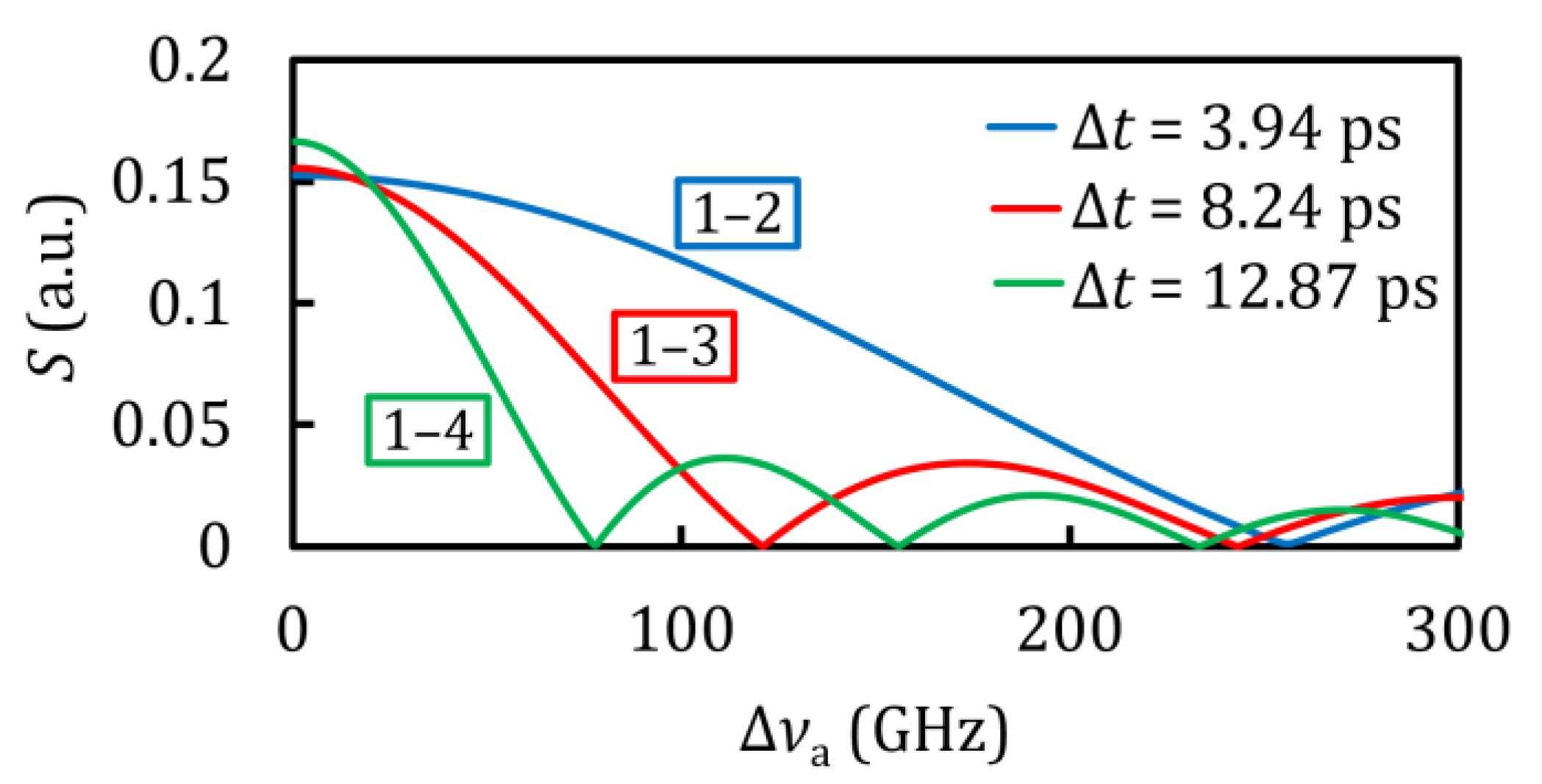
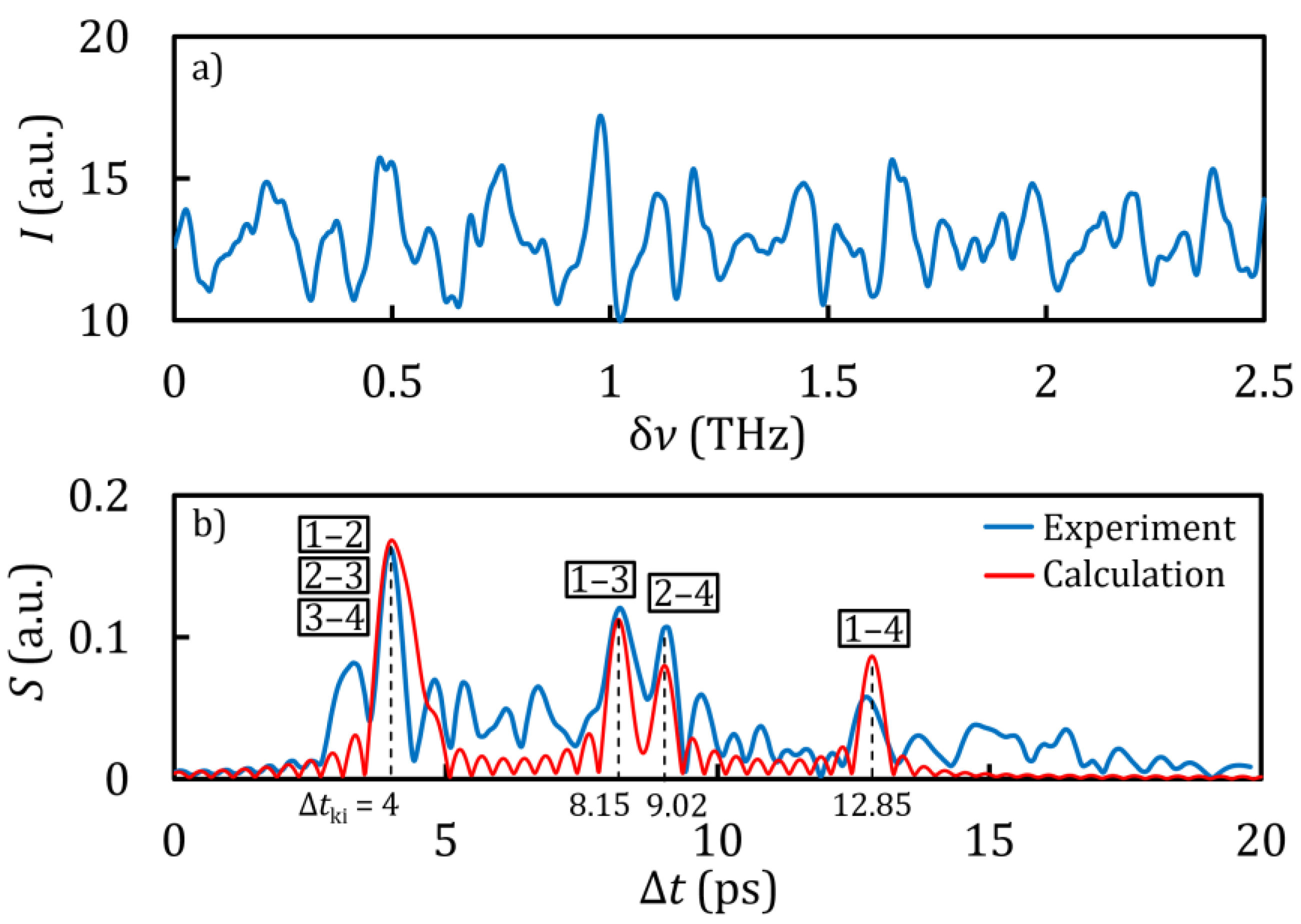
• The phase change of the selected spectral component was determined (one of the 4 spectral components shown in Figure 8b). The value of the Fourier image argument for the selected spectral component was treated as the phase of the spectral component.
• A phase unwrap algorithm was used to obtain the continuous phase dependence on the magnitude of the EFP.
• The magnitude of the EFP was related to the magnitude of the phase change, so the phase change being the effect of the EFP can be considered as an IFI response.

Figure 10 shows the IFISI response obtained on the spectral component with Δt = 8.15 ps (a pair of mode groups with indices 1–3). It can be seen that the shape of the response at a large magnitude of the EFP corresponds to the shape of the EFP. In the case of an EFP with small magnitude, the shape of the response is noticeably distorted as a result of the influence of noise.

Figure 11 shows the experimentally obtained dependence of the Root Mean Square (RMS) value of the IFISI response on the EFP magnitude. It can be seen that the experimentally obtained dependence is in good agreement with the dependence obtained as a result of calculation by Equation (4).

It can be seen from Figure 11 that the approach of obtaining the IFISI response to EFP, based on Fourier analysis of IFISI signals, provides determination of EFP in a large dynamic range. In fact, the dynamic range is limited only by the intrinsic noise of the interrogator and inevitable optical noise.

To confirm this conclusion, these noises were estimated for all three spectral components (the RMS value of the phase change amplitude of the corresponding spectral component in the absence of EFP was adopted as the noise level). It can be seen that the magnitude of the IFISI response in the case of small EFP magnitude (at δL < 1 µm) corresponds to the noise level.

Thus, it can be seen that the method of determining the phase of the spectral component of the Fourier image of the STF allows us to obtain a linear response to EFP in a wide dynamic range.

We will now discuss the limitations of the dynamic range of the IFISI with Fourier analysis of its signals.

In the case of small EFP magnitudes, the linearity of the IFISI response is limited mainly by noise resulting from the influence of intrinsic noise of the interrogator and optical noise (mode noise, noise associated with the occurrence of a parasitic Fabry–Perot interferometer in FC/PC connectors, etc.).

Also, a necessary procedure for achieving a linear response in a wide dynamic range consists in the use of a phase unwrapping algorithm. Firstly, large-amplitude EFP can lead to a situation where the magnitude of the change in phase difference of the selected pair of mode groups caused by EFP exceeds 2π. This leads to phase discontinuities in the IFISI’s response, which need to be eliminated using a phase unwrapping algorithm. Secondly, if the initial phase difference of the selected pair of mode groups is close to π or −π, phase discontinuities can occur even if the magnitude of the phase difference change caused by EFP is less than 2π. To obtain a linear response in this case, it is necessary to apply a phase unwrapping algorithm as well.

Thus, in this section, we experimentally validated the results obtained in the theoretical section. We demonstrated that the IFISI’s STF contains information about the composition of the excited mode groups in the MMF. Therefore, the experimental measurement of the STF and the application of the developed mathematical model allow us to determine the number of mode groups, their relative amplitudes, and the delay times between the mode groups. We also measured the IFISI’s response to EFP (the MMF length modulation according to the harmonic law with a frequency of 0.5 Hz and a magnitude ranging from 0.1 to 220 µm) and compared the results with the calculations based on the developed mathematical model. As a result, our research has confirmed that the IFISI with Fourier analysis of its signals provides a linear response to EFP in a wide dynamic range.

4. Conclusions

This article presents the results of a theoretical and experimental study of the approach of applying Fourier analysis to IFISI signals to measure EFP. A mathematical model was developed that takes into account the main parameters of the IFISI (MMF parameters, optical frequency scanning parameters, and number of excited mode groups). Calculations of STFs and Fourier images for various parameters of the IFISI were carried out in order to identify the values of these parameters that ensure the optimal operation of the measuring circuit. It is also shown that the developed mathematical model makes it possible to determine such parameters of an intermodal fiber interferometer as the number of excited mode groups, their relative amplitudes, and the delay times between the mode groups.

The considered approach was implemented experimentally. It has been shown that this approach makes it possible to obtain a linear response to EFP in a wide dynamic range.

The results of the experiment were also compared with the results of calculations based on the developed mathematical model. The calculation results are consistent with the experimental results, which allows us to conclude that the proposed mathematical model is physically correct.

In this article, a method for implementing spectral interrogation of IFIs using a laser with optical frequency scanning is considered. However, spectral interrogation using a broadband light source and an optical spectrum analyzer can also be used to implement the approach of Fourier analysis of IFISI signals discussed in this article. It is notable that for this method of spectral interrogation, the mathematical model presented in this article is also applicable. It is important to note that for this variant of spectral interrogation, instead of the parameter characterizing the laser linewidth, it is necessary to use the parameter characterizing the width of the instrumental function of the optical spectrum analyzer. The remaining statements of the mathematical model are identical for both spectral interrogation methods.

The results of the present work incontestably prove that the IFISI-based EFP sensors enable a linear response over a wide dynamic range of external fiber perturbations.

References

1. Pevec, S.; Donlagić, D. Multiparameter Fiber-Optic Sensors: A Review. Opt. Eng. 2019, 58, 072009. [Google Scholar] [CrossRef]
2. Zhu, Z.; Ba, D.; Liu, L.; Qiu, L.; Yang, S.; Dong, Y. Multiplexing of Fabry-Pérot Sensor by Frequency Modulated Continuous Wave Interferometry for Quais-Distributed Sensing Application. J. Light. Technol. 2021, 39, 4529–4534. [Google Scholar] [CrossRef]
3. Hartog, A.H. An Introduction to Distributed Optical Fibre Sensors; CRC Press: Boca Raton, FL, USA, 2017; ISBN 9781315119014. [Google Scholar]
4. Reyes-Vera, E.; Cordeiro, C.M.B.; Torres, P. Highly Sensitive Temperature Sensor Using a Sagnac Loop Interferometer Based on a Side-Hole Photonic Crystal Fiber Filled with Metal. Appl. Opt. 2017, 56, 156. [Google Scholar] [CrossRef] [PubMed]
5. Zhao, Y.; Chen, M.; Xia, F.; Lv, R. Small In-Fiber Fabry-Perot Low-Frequency Acoustic Pressure Sensor with PDMS Diaphragm Embedded in Hollow-Core Fiber. Sens. Actuators A. Phys. 2018, 270, 162–169. [Google Scholar] [CrossRef]
6. Wang, K.; Dong, X.; Kohler, M.H.; Kienle, P.; Bian, Q.; Jakobi, M.; Koch, A.W. Advances in Optical Fiber Sensors Based on Multimode Interference (MMI): A Review. IEEE Sens. J. 2021, 21, 132–142. [Google Scholar] [CrossRef]
7. Leal-Junior, A.G.; Theodosiou, A.; Diaz, C.R.; Marques, C.; Pontes, M.J.; Kalli, K.; Frizera, A. Simultaneous Measurement of Axial Strain, Bending and Torsion With a Single Fiber Bragg Grating in CYTOP Fiber. J. Light. Technol. 2019, 37, 971–980. [Google Scholar] [CrossRef]
8. Mizuno, Y.; Theodosiou, A.; Kalli, K.; Liehr, S.; Lee, H.; Nakamura, K. Distributed Polymer Optical Fiber Sensors: A Review and Outlook. Photonics Res. 2021, 9, 1719. [Google Scholar] [CrossRef]
9. Newaz, A.; Faruque, M.O.; Al Mahmud, R.; Sagor, R.H.; Khan, M.Z.M. Machine-Learning-Enabled Multimode Fiber Specklegram Sensors: A Review. IEEE Sens. J. 2023, 23, 20937–20950. [Google Scholar] [CrossRef]
10. Pang, Y.-N.; Liu, B.; Liu, J.; Wan, S.-P.; Wu, T.; Yuan, J.; Xin, X.; He, X.-D.; Wu, Q. Singlemode-Multimode-Singlemode Optical Fiber Sensor for Accurate Blood Pressure Monitoring. J. Light. Technol. 2022, 40, 4443–4450. [Google Scholar] [CrossRef]
11. Li, G.; Liu, Y.; Qin, Q.; Pang, L.; Ren, W.; Wei, J.; Wang, M. Fiber Specklegram Torsion Sensor Based on Residual Network. Opt. Fiber Technol. 2023, 80, 103446. [Google Scholar] [CrossRef]
12. Lomer, M.; Rodriguez-Cobo, L.; Revilla, P.; Herrero, G.; Madruga, F.; Lopez-Higuera, J.M. Speckle POF Sensor for Detecting Vital Signs of Patients. In Proceedings of the SPIE—The International Society for Optical Engineering, Santander, Spain, 2 June 2014. [Google Scholar] [CrossRef]
13. Chen, W.; Feng, F.; Chen, D.; Lin, W.; Chen, S.-C. Precision Non-Contact Displacement Sensor Based on the near-Field Characteristics of Fiber Specklegrams. Sens. Actuators A. Phys. 2019, 296, 1–6. [Google Scholar] [CrossRef]
14. Varyshchuk, V.; Bobitski, Y.; Poisel, H. Deformation Sensing with a Multimode POF Using Speckle Correlation Processing Method. Opto-Electron. Rev. 2017, 25, 19–23. [Google Scholar] [CrossRef]
15. Feng, F.; Chen, W.; Chen, D.; Lin, W.; Chen, S.-C. In-Situ Ultrasensitive Label-Free DNA Hybridization Detection Using Optical Fiber Specklegram. Sens. Actuators B. Chem. 2018, 272, 160–165. [Google Scholar] [CrossRef]
16. Chapalo, I.; Stylianou, A.; Mégret, P.; Theodosiou, A. Advances in Optical Fiber Speckle Sensing: A Comprehensive Review. Photonics 2024, 11, 299. [Google Scholar] [CrossRef]
17. Efendioglu, H.S. A Review of Fiber-Optic Modal Modulated Sensors: Specklegram and Modal Power Distribution Sensing. IEEE Sens. J. 2017, 17, 2055–2064. [Google Scholar] [CrossRef]
18. Wang, K.; Mizuno, Y.; Dong, X.; Kurz, W.; Köhler, M.; Kienle, P.; Lee, H.; Jakobi, M.; Koch, A.W. Multimode Optical Fiber Sensors: From Conventional to Machine Learning-Assisted. Meas. Sci. Technol. 2024, 35, 022002. [Google Scholar] [CrossRef]
19. Guzmán-Sepúlveda, J.R.; Guzmán-Cabrera, R.; Castillo-Guzmán, A.A. Optical Sensing Using Fiber-Optic Multimode Interference Devices: A Review of Nonconventional Sensing Schemes. Sensors 2021, 21, 1862. [Google Scholar] [CrossRef] [PubMed]
20. Li, G.; Liu, Y.; Qin, Q.; Zou, X.; Wang, M.; Ren, W. Feature Extraction Enabled Deep Learning From Specklegram for Optical Fiber Curvature Sensing. IEEE Sens. J. 2022, 22, 15974–15984. [Google Scholar] [CrossRef]
21. Wang, X.; Song, L.; Wang, X.; Lu, S.; Li, J.; Zhang, P.; Fang, F. An Ultrasensitive Fiber-End Tactile Sensor With Large Sensing Angle Based on Specklegram Analysis. IEEE Sens. J. 2023, 23, 30394–30402. [Google Scholar] [CrossRef]
22. Wang, X.; Yang, Y.; Li, S.; Wang, X.; Zhang, P.; Lu, S.; Yu, D.; Zheng, Y.; Song, L.; Fang, F. A Reflective Multimode Fiber Vector Bending Sensor Based on Specklegram. Opt. Laser Technol. 2024, 170, 110235. [Google Scholar] [CrossRef]
23. Mizuno, Y.; Numata, G.; Kawa, T.; Lee, H.; Hayashi, N.; Nakamura, K. Multimodal Interference in Perfluorinated Polymer Optical Fibers: Application to Ultrasensitive Strain and Temperature Sensing. IEICE Trans. Electron. 2018, 101, 602–610. [Google Scholar] [CrossRef]
24. Chapalo, I.; Theodosiou, A.; Kalli, K.; Kotov, O. Multimode Fiber Interferometer Based on Graded-Index Polymer CYTOP Fiber. J. Light. Technol. 2020, 38, 1439–1445. [Google Scholar] [CrossRef]
25. Fan, X.; Jiang, J.; Zhang, X.; Liu, K.; Wang, S.; Liu, T. Multimode Interferometer-Based Torsion Sensor Employing Perfluorinated Polymer Optical Fiber. Opt. Express 2019, 27, 28123. [Google Scholar] [CrossRef] [PubMed]
26. Fujiwara, E.; Evaristo da Silva, L.; Marques, T.H.R.; Cordeiro, C.M.B. Polymer Optical Fiber Specklegram Strain Sensor with Extended Dynamic Range. Opt. Eng. 2018, 57, 116107. [Google Scholar] [CrossRef]
27. Theodosiou, A. Adaptive Refractive Index Measurements via Polymer Optical Fiber Speckle Pattern Analysis. IEEE Sens. J. 2024, 24, 287–291. [Google Scholar] [CrossRef]
28. Silva, S.; Frazão, O.; Viegas, J.; Ferreira, L.A.; Araújo, F.M.; Malcata, F.X.; Santos, J.L. Temperature and Strain-Independent Curvature Sensor Based on a Singlemode/Multimode Fiber Optic Structure. Meas. Sci. Technol. 2011, 22, 085201. [Google Scholar] [CrossRef]
29. Lu, C.; Su, J.; Dong, X.; Sun, T.; Grattan, K.T.V. Simultaneous Measurement of Strain and Temperature With a Few-Mode Fiber-Based Sensor. J. Light. Technol. 2018, 36, 2796–2802. [Google Scholar] [CrossRef]
30. Markvart, A.A.; Liokumovich, L.B.; Ushakov, N.A. Fiber Optic SMS Sensor for Simultaneous Measurement of Strain and Curvature. Tech. Phys. Lett. 2022, 48, 30. [Google Scholar] [CrossRef]
31. Kotov, O.I.; Kosareva, L.I.; Liokumovich, L.B.; Markov, S.I.; Medvedev, A.V.; Nikolaev, V.M. Multichannel Signal Detection in a Multimode Optical-Fiber Interferometer: Ways to Reduce the Effect of Amplitude Fading. Tech. Phys. Lett. 2000, 26, 844–848. [Google Scholar] [CrossRef]
32. Kotov, O.I.; Bisyarin, M.A.; Chapalo, I.E.; Petrov, A.V. Simulation of a Multimode Fiber Interferometer Using Averaged Characteristics Approach. J. Opt. Soc. Am. B 2018, 35, 1990. [Google Scholar] [CrossRef]
33. Chapalo, I.; Petrov, A.; Bozhko, D.; Bisyarin, M.; Kotov, O. Averaging Methods for a Multimode Fiber Interferometer: Experimental and Interpretation. J. Light. Technol. 2020, 38, 5809–5816. [Google Scholar] [CrossRef]
34. Rodríguez-Cuevas, A.; Peña, E.R.; Rodríguez-Cobo, L.; Lomer, M.; Higuera, J.M.L. Low-Cost Fiber Specklegram Sensor for Noncontact Continuous Patient Monitoring. J. Biomed. Opt. 2017, 22, 037001. [Google Scholar] [CrossRef] [PubMed]
35. Rodriguez-Cobo, L.; Lomer, M.; Lopez-Higuera, J.-M. Fiber Specklegram-Multiplexed Sensor. J. Light. Technol. 2015, 33, 2591–2597. [Google Scholar] [CrossRef]
36. Fujiwara, E.; Ri, Y.; Wu, Y.T.; Fujimoto, H.; Suzuki, C.K. Evaluation of Image Matching Techniques for Optical Fiber Specklegram Sensor Analysis. Appl. Opt. 2018, 57, 9845. [Google Scholar] [CrossRef]
37. Liu, Y.; Qin, Q.; Liu, H.; Tan, Z.; Wang, M. Investigation of an Image Processing Method of Step-Index Multimode Fiber Specklegram and Its Application on Lateral Displacement Sensing. Opt. Fiber Technol. 2018, 46, 48–53. [Google Scholar] [CrossRef]
38. Fujiwara, E.; Marques dos Santos, M.F.; Suzuki, C.K. Optical Fiber Specklegram Sensor Analysis by Speckle Pattern Division. Appl. Opt. 2017, 56, 1585. [Google Scholar] [CrossRef] [PubMed]
39. Osório, J.H.; Cabral, T.D.; Fujiwara, E.; Franco, M.A.R.; Amrani, F.; Delahaye, F.; Gérôme, F.; Benabid, F.; Cordeiro, C.M.B. Displacement Sensor Based on a Large-Core Hollow Fiber and Specklegram Analysis. Opt. Fiber Technol. 2023, 78, 103335. [Google Scholar] [CrossRef]
40. Zhao, F.; Lin, W.; Guo, P.; Hu, J.; Liu, S.; Yu, F.; Zuo, G.; Wang, G.; Liu, H.; Chen, J.; et al. Demodulation of DBR Fiber Laser Sensors With Speckle Patterns. IEEE Sens. J. 2023, 23, 26022–26030. [Google Scholar] [CrossRef]
41. Zain, M.A.; Karimi-Alavijeh, H.; Moallem, P.; Khorsandi, A.; Ahmadi, K. A High-Sensitive Fiber Specklegram Refractive Index Sensor With Microfiber Adjustable Sensing Area. IEEE Sens. J. 2023, 23, 15570–15577. [Google Scholar] [CrossRef]
42. Liu, Y.; Lin, W.; Zhao, F.; Liu, Y.; Sun, J.; Hu, J.; Li, J.; Chen, J.; Zhang, X.; Vai, M.I.; et al. A Multimode Microfiber Specklegram Biosensor for Measurement of CEACAM5 through AI Diagnosis. Biosens. 2024, 14, 57. [Google Scholar] [CrossRef]
43. Inalegwu, O.C.; II, R.E.G.; Huang, J. A Machine Learning Specklegram Wavemeter (MaSWave) Based on a Short Section of Multimode Fiber as the Dispersive Element. Sensors 2023, 23, 4574. [Google Scholar] [CrossRef] [PubMed]
44. Jiang, Y.; Ding, W. Recent Developments in Fiber Optic Spectral White-Light Interferometry. Photonic Sens. 2011, 1, 62–71. [Google Scholar] [CrossRef]
45. Liu, W.; Ren, Q.; Jia, P.; Hong, Y.; Liang, T.; Liu, J.; Xiong, J. Least Square Fitting Demodulation Technique for the Interrogation of an Optical Fiber Fabry–Perot Sensor with Arbitrary Reflectivity. Appl. Opt. 2020, 59, 1301. [Google Scholar] [CrossRef]
46. Rota-Rodrigo, S.; Lopez-Aldaba, A.; Perez-Herrera, R.A.; del Carmen Lopez Bautista, M.; Esteban, O.; Lopez-Amo, M. Simultaneous Measurement of Humidity and Vibration Based on a Microwire Sensor System Using Fast Fourier Transform Technique. J. Light. Technol. 2016, 34, 4525–4530. [Google Scholar] [CrossRef]
47. Yu, Z.; Wang, A. Fast White Light Interferometry Demodulation Algorithm for Low-Finesse Fabry–Pérot Sensors. IEEE Photonics Technol. Lett. 2015, 27, 817–820. [Google Scholar] [CrossRef]
48. Yu, Z.; Wang, A. Fast Demodulation Algorithm for Multiplexed Low-Finesse Fabry–Pérot Interferometers. J. Light. Technol. 2016, 34, 1015–1019. [Google Scholar] [CrossRef]
49. Wong, K.P.; Kim, H.-T.; Rajasekaran, K.; Yazdkhasti, A.; Sai Sudhakar, B.; Wang, A.; Lee, S.E.; Kiger, K.; Duncan, J.H.; Yu, M. High-Speed, Large Dynamic Range Spectral Domain Interrogation of Fiber-Optic Fabry–Perot Interferometric Sensors. Appl. Opt. 2022, 61, 4670. [Google Scholar] [CrossRef] [PubMed]
50. Jassam, G.M.; Ahmed, S.S. Tapered PCF Mach–Zehnder Interferometer Based on Surface Plasmon Resonance (SPR) for Estimating Concentration Toxic Metal Ions (Lead). J. Opt. 2024, 53, 163–168. [Google Scholar] [CrossRef]
51. Cardona-Maya, Y.; Del Villar, I.; Socorro, A.B.; Corres, J.M.; Matias, I.R.; Botero-Cadavid, J.F. Wavelength and Phase Detection Based SMS Fiber Sensors Optimized With Etching and Nanodeposition. J. Light. Technol. 2017, 35, 3743–3749. [Google Scholar] [CrossRef]
52. Ushakov, N.; Markvart, A.; Liokumovich, L. Singlemode-Multimode-Singlemode Fiber-Optic Interferometer Signal Demodulation Using MUSIC Algorithm and Machine Learning. Photonics 2022, 9, 879. [Google Scholar] [CrossRef]
53. Galarza, M.; Perez-Herrera, R.A.; Leandro, D.; Judez, A.; López-Amo, M. Spatial-Frequency Multiplexing of High-Sensitivity Liquid Level Sensors Based on Multimode Interference Micro-Fibers. Sens. Actuators A Phys. 2020, 307, 111985. [Google Scholar] [CrossRef]
54. Álvarez-Tamayo, R.; Durán-Sánchez, M.; Prieto-Cortés, P.; Salceda-Delgado, G.; Castillo-Guzmán, A.; Selvas-Aguilar, R.; Ibarra-Escamilla, B.; Kuzin, E. All-Fiber Laser Curvature Sensor Using an In-Fiber Modal Interferometer Based on a Double Clad Fiber and a Multimode Fiber Structure. Sensors 2017, 17, 2744. [Google Scholar] [CrossRef] [PubMed]
55. Wu, Q.; Qu, Y.; Liu, J.; Yuan, J.; Wan, S.-P.; Wu, T.; He, X.-D.; Liu, B.; Liu, D.; Ma, Y.; et al. Singlemode-Multimode-Singlemode Fiber Structures for Sensing Applications—A Review. IEEE Sens. J. 2021, 21, 12734–12751. [Google Scholar] [CrossRef]
56. Petrov, A.V.; Chapalo, I.E.; Bisyarin, M.A.; Kotov, O.I. Intermodal Fiber Interferometer with Frequency Scanning Laser for Sensor Application. Appl. Opt. 2020, 59, 10422. [Google Scholar] [CrossRef] [PubMed]
57. Petrov, A.V.; Bisyarin, M.A.; Kotov, O.I. Broadband Intermodal Fiber Interferometer for Sensor Application: Fundamentals and Simulator. Appl. Opt. 2022, 61, 6544. [Google Scholar] [CrossRef]
58. Gowar, J. Optical Communication Systems; Prentice-Hall, Inc.: Englewood Cliffs, NJ, USA, 1993. [Google Scholar]
59. Korn, G.A.; Korn, T.M. Mathematical Handbook for Scientists and Engineers: Definitions, Theorems, and Formulas for Reference and Review; Courier Corporation: North Chelmsford, MA, USA, 2000. [Google Scholar]
Figure 1. Illustration of the IFISI operating principle. (a) Schematic of an IFISI; (b) dependence of the MMF elongation value δL on time (EFP); (c) time sequence of optical frequency scans; (d) STFs obtained at δL = 0 µm, δL = 100 µm, and δL = 200 µm on an enlarged time scale; (e) the STFs obtained at δL = 0 µm, δL = 100 µm, and δL = 200 µm plotted on a single graph. The detuning of the optical frequency δν from the optical frequency ν0 is postponed along the abscissa axis.
Photonics 11 00423 g001
Figure 2. (ac) STFs calculated using Equation (2) for a different number of excited mode groups M. In graph (c), the STF shift as a result of EFP δL = 300 µm is additionally plotted. (df) The moduli of the Fourier images of the STF calculated using Equation (4) for a different number of excited mode groups M. For each spectral component, it is indicated which pair of mode groups it corresponds to. Calculation parameters: optical frequency scanning range Δνspan = 5 THz, other parameters according to Table 1.
Photonics 11 00423 g002
Figure 3. STF obtained by scanning the optical frequency in the range Δνspan = 1 THz (a) and the moduli of the Fourier images of the STF obtained for the optical frequency scanning range Δνspan = 10 THz (b) for different refractive index profiles. Calculation parameters: MMF length L = 25 m, number of mode groups M = 3, other parameters according to Table 1.
Photonics 11 00423 g003
Figure 4. The dependences of the magnitudes of the three spectral components of the modulus of the Fourier image on the laser linewidth Δνa. Above each curve, it is indicated which pair of mode groups it corresponds to. Calculation parameters: optical frequency scanning range Δνspan = 10 THz, number of mode groups M = 4, other parameters according to Table 1.
Photonics 11 00423 g004
Figure 5. The moduli of the Fourier images of the STF calculated using Equation (4) for different optical frequency scanning ranges Δνspan, (a) Δνspan = 10 THz and (b) Δνspan = 2.5 THz. For each spectral component, it is indicated which pair of mode groups it corresponds to. Calculation parameters: the number of mode groups M = 4, the remaining parameters according to Table 1.
Photonics 11 00423 g005
Figure 6. The dependence of the argument of the spectral component of the Fourier image on the magnitude of the EFP. For each line, it is indicated which pair of mode groups it corresponds to. Calculation parameters: optical frequency scanning range Δνspan = 10 THz, other parameters according to Table 1.
Photonics 11 00423 g006
Figure 7. The scheme of the experimental setup: (1)—Interrogator NI PXIe 4844; (2)—Optical circulator; (3) and (5)—FC/PC connector; (4)—Piezoceramic modulator.
Photonics 11 00423 g007
Figure 8. (a) The experimental STF obtained by scanning the optical frequency in the range Δνspan = 2.5 THz; (b) the modulus of Fourier images of the experimentally obtained STF and the modulus of Fourier images calculated by Equation (4). For each spectral component, it is indicated which pair of mode groups it corresponds to. Calculation parameters: optical frequency scanning range Δνspan = 2.5 THz, number of mode groups M = 4, other parameters according to Table 1.
Photonics 11 00423 g008
Figure 9. Experimentally obtained (solid lines) and simulated (dotted lines) dependences of the magnitudes of the three spectral components of the Fourier image on the laser linewidth Δνa. Calculation parameters: optical frequency scanning range Δνspan = 2.5 THz, number of mode groups M = 4, other parameters according to Table 1.
Photonics 11 00423 g009
Figure 10. The IFISI response (phase change of the spectral component with Δt = 8.15 ps) obtained for two different EFP magnitudes.
Photonics 11 00423 g010
Figure 11. The experimentally obtained dependence of the RMS value of the IFISI response on the EFP magnitude (dots) and the dependence obtained as a result of calculation using Equation (4) (solid lines). The dotted lines indicate the noise level, which was defined as the RMS value of the phase change amplitude of the corresponding spectral component in the absence of EFP. Calculation parameters: optical frequency scanning range Δνspan = 2.5 THz, number of mode groups M = 4, other parameters according to Table 1.
Photonics 11 00423 g011