Effects of Squeezing on the Power Broadening and Shifts of Micromaser Lineshapes

Abstract

AC Stark shifts have an impact on the dynamics of atoms interacting with a near-resonant quantized single-mode cavity field, which is relevant to a single atom micromaser. In this study, we demonstrate that, when the field is in a squeezed coherent state, atomic lineshapes are highly sensitive to the squeezing parameter. Furthermore, we show that, when considering a superposition of squeezed coherent states with equal amplitude, the displacement of the transition lines depends significantly, not only on the squeezing parameter, but also on its sign.

1. Introduction

Major steps towards the generation of nonclassical states of the quantized electromagnetic field have been taken over the years. Nonclassical states usually exhibit less fluctuations or noise than coherent states [1,2] for certain observables; for this reason, noise associated with coherent states is referred to as the standard quantum limit. Among the nonclassical states that have attracted much interest over the years are squeezed states, states that are known to produce notable effects in the atomic inversion and in the resonance fluorescence spectrum of a two-level atom, because the shape of the photon distribution (which may be very different from that of a coherent state) is directly reflected in both the atomic inversion and the atomic spectrum. Such a photon distribution imprints its signature in the atomic inversion, producing the so-called “ringing revivals” [3,4]. Squeezed states are also of great importance in cases where the detection of light needs to be extremely efficient, such as in gravitational wave detectors; in fact, gravitational wave interferometers obtain their great sensitivity by combining suspended masses and squeezed states of light [5,6,7].

On the other hand, in experimental studies of micromasers [8], asymmetries and Stark shifts in lineshapes have been observed and attributed to the effects of nearby off-resonant levels [9]. In fact, there have been attempts to explain the lineshapes of conventional lasers with frequency fluctuations or external noises [10], and practical laser linewidth broadening phenomenon in lasers have been presented [11]. Such lineshapes may be affected by the photon distribution of the quantized field; in particular, for a number state, the AC Stark shift moves the power-broadened resonance away from its unperturbed value; however, for a field with many contributions to the photon number, the distinct distribution of shifts contributes to a mean shift and to an effective broadening of the resonance [12]. Micromaser lineshapes are very sensitive to the temperature at which the micromaser is operated, and at lower temperatures thermal asymmetries become much less significant [13,14].

The effects of nearby levels can also be observed in the resonance fluorescence spectrum, where the Stark shift created by such levels produces displacements of the resonance fluorescence peaks, because of an induced effective detuning [15,16]. In fact, it has been shown that the AC Stark effect can influence the transfer of quantum entangled information [17]. In addition, a Doppler-free absorptive lineshape has been formulated for coherently prepared drive–probe systems, where the individual contributions of the drive and probe fields to AC Stark splitting can be demonstrated by the broadening of lineshapes [18]. Comparison between the AC Stark effects and the effects produced by nonlinear interactions, namely, the Kerr interaction, has been carried out [19]. Brune et al. [20] showed that intensity-dependent Stark shifts may be employed in quantum non-demolition measurements of the cavity photon numbers in micromasers.

The primary aim and motivation of this work is to study how the squeezing parameter affects atomic lineshapes, within the framework of the Jaynes–Cummings model with the AC Stark term, while considering nearby non-resonant levels. The structure of the article is as follows: In Section 2, we solve the Schrödinger equation and examine specific cases in which the atom is initially in either its first excited state or its ground state. Using a squeezed coherent state as the initial condition for the field, in Section 3, we analyze the effects of nearby non-resonant levels on atomic inversion and demonstrate how the lineshapes are distorted and broadened as the squeezing parameter r varies. In Section 4, we extend the analysis to a superposition of squeezed coherent states with the same atomic conditions as in Section 3. We show that the changes in the lineshapes are highly sensitive, not only to the amplitude of the squeezing parameter, but also to its sign. In Section 5, we briefly discuss our results and finally, in Section 6, we present our conclusions.

2. AC Stark Shift Hamiltonian

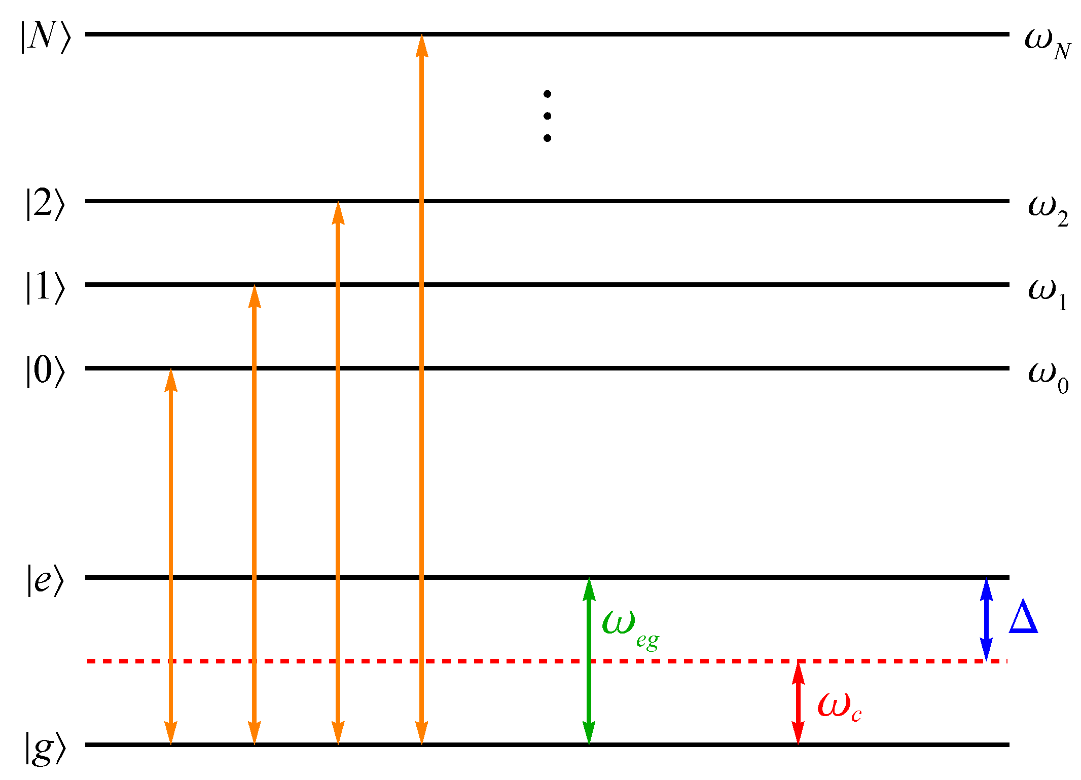
Let us consider an atom with a ground state $|g⟩$, an excited state $|e⟩$, and higher states denoted by $|j⟩$, with $j=0,1,2,\dots N$. The atom interacts with a single-mode field, as shown in Figure 1. We consider that the field is approximately tuned to the transition frequency between the levels $|g⟩$ and $|e⟩$ of the atom, but detuned from the nearby levels $|j⟩$ (AC Stark effect). The Hamiltonian that describes this system is [9,12,15,21]

$$\widehat{H}=\frac{{\omega }_{eg}}{2}{\widehat{\sigma }}_z+{\omega }_c{\widehat{a}}^{†}\widehat{a}+\chi {\widehat{a}}^{†}\widehat{a}{\widehat{\sigma }}_z+g\left({\widehat{\sigma }}_{+}\widehat{a}+{\widehat{\sigma }}_{-}{\widehat{a}}^{†}\right),$$

(1)

where g is the coupling constant between the two-level system and the field (in the dipole approximation and in the rotating wave approximation), while $\chi$ is the parameter that quantifies the intensity of the interaction in the AC Stark effect, due to the presence of nearby non-resonant virtual levels. Creation and annihilation operators, ${\widehat{a}}^{†}$ and $\widehat{a}$, are used, which satisfy the commutation relation $\left[\widehat{a},{\widehat{a}}^{†}\right]=1$. Additionally, to describe the atomic part of the system, we use the operators ${\widehat{\sigma }}_{+}=|e⟩⟨g|$, ${\widehat{\sigma }}_{-}=|g⟩⟨e|$, and ${\widehat{\sigma }}_z=|e⟩⟨e|-|g⟩⟨g|$, which satisfy the commutation relations $[{\widehat{\sigma }}_{+},{\widehat{\sigma }}_{-}]={\widehat{\sigma }}_z$ and $[{\widehat{\sigma }}_z,{\widehat{\sigma }}_{\pm }]=\pm 2{\widehat{\sigma }}_{\pm }$.

Figure 1. Energy level diagram showing the pair of nearly resonant excited atomic states with transition frequency ${\omega }_{eg}$, the field frequency ${\omega }_c$, and a set of non-resonant levels that only participate virtually in the excitation and are responsible for the AC Stark shifts at the transition frequency ${\omega }_{eg}$.

We proceed to an interaction picture moving to a frame that rotates at frequency ${\omega }_c$; i.e., by means of the time-dependent unitary transformation $\widehat{\mathcal{R}}=exp\left[\mathrm{i}{\omega }_{c}t(\widehat{n}+{\widehat{\sigma }}_z/2)\right]$, to produce the Schrödinger equation

$$\mathrm{i}\frac{d|\mathrm{\Psi }\left(t\right)⟩}{dt}=\widehat{\mathcal{H}}|\mathrm{\Psi }\left(t\right)⟩,$$

(2)

with the interaction Hamiltonian

$$\begin{array}{cc}\hfill \widehat{\mathcal{H}}& =\widehat{\mathcal{R}}\widehat{H}{\widehat{\mathcal{R}}}^{†}-\mathrm{i}\widehat{\mathcal{R}}{\partial }_t{\widehat{\mathcal{R}}}^{†},\hfill \\ \hfill & =\left(\frac{\Delta }{2}+\chi \widehat{n}\right){\widehat{\sigma }}_z+g\left({\widehat{\sigma }}_{+}\widehat{a}+{\widehat{\sigma }}_{-}{\widehat{a}}^{†}\right),\hfill \end{array}$$

(3)

being $\Delta ={\omega }_{eg}-{\omega }_c$ the detuning between the field frequency and the atomic transition frequency, and $\widehat{n}={\widehat{a}}^{†}\widehat{a}$ the usual number operator [22,23,24,25,26,27,28,29] of the field.

From the Hamiltonian $\widehat{\mathcal{H}}$, the dynamics of any initial condition can be obtained by solving the Schrödinger Equation (2) by one of the known methods [23,24,25,26,27,28,29]. In this work, we use the traditional method that proposes that at time t the atom-field state vector is a superposition of Fock states $\left\{|n⟩\right\}$. Given that only two (composed) levels are coupled by the above Hamiltonian, namely $|n⟩|e⟩$ and $|n+1⟩|g⟩$, we may write the solution as

$$|\mathrm{\Psi }\left(t\right)⟩=\sum _{n=0}^{\infty }\left[C_n\left(t\right)|n⟩|e⟩+D_n\left(t\right)|n+1⟩|g⟩\right],$$

(4)

where the coefficients $C_n\left(t\right)$ and $D_n\left(t\right)$ are to be determined; in order to do so, we insert this proposal into the Schrödinger Equation (2), and the problem is reduced to solving the system of coupled differential equations

$$\mathrm{i}\frac{d}{dt}\left(\begin{array}{c}{C}_n\left(t\right)\\ D_n\left(t\right)\end{array}\right)=\left(\begin{array}{cc}\chi n+\frac{\Delta }{2}& g\sqrt{n+1}\\ g\sqrt{n+1}& -\chi (n+1)-\frac{\Delta }{2}\end{array}\right)\left(\begin{array}{c}{C}_n\left(t\right)\\ D_n\left(t\right)\end{array}\right),n=0,1,2,\dots .$$

(5)

The general solution of these differential equations is

$$\left(\begin{array}{c}{C}_n\left(t\right)\\ D_n\left(t\right)\end{array}\right)=exp\left(\mathrm{i}\frac{\chi t}{2}\right)\left(\begin{array}{cc}{M}_{11}\left(t\right)& M_{12}\left(t\right)\\ M_{21}\left(t\right)& M_{22}\left(t\right)\end{array}\right)\left(\begin{array}{c}{C}_n\left(0\right)\\ D_n\left(0\right)\end{array}\right),n=0,1,2,\dots ,$$

(6)

where

$$\begin{array}{cc}\hfill M_{11}\left(t\right)& =cos\left(\frac{{\beta }_{n}t}{2}\right)-\mathrm{i}\frac{\Delta +\chi (2n+1)}{{\beta }_n}sin\left(\frac{{\beta }_{n}t}{2}\right),\hfill \\ \hfill M_{12}\left(t\right)& =-\mathrm{i}\frac{2g\sqrt{n+1}}{{\beta }_n}sin\left(\frac{{\beta }_{n}t}{2}\right),\hfill \\ \hfill M_{22}\left(t\right)& =M_{11}^{\ast }\left(t\right),M_{21}\left(t\right)=M_{12}\left(t\right),n=0,1,2,\dots .\hfill \end{array}$$

(7)

The quantities $|C_n{\left(0\right)|}^2$ and $|D_n{\left(0\right)|}^2$ determine the initial distribution of photons in the excited and ground states of the atom, respectively. Meanwhile, ${\beta }_n$ is the generalized Rabi frequency caused by AC Stark shifts; these shifts correspond to variations in the energy of an atom resulting from the presence of a non-resonant electric field. The expression for ${\beta }_n$ is

$${\beta }_n=\sqrt{{\left[\Delta +\chi (2n+1)\right]}^2+4g^2(n+1)},n=0,1,2,\dots .$$

(8)

Once the initial atom-field condition $|\mathrm{\Psi }\left(0\right)⟩$ is given, it is possible to obtain the temporal evolution of any observable of the system. In this case, we focus on atomic inversion, $W\left(t\right)=⟨\mathrm{\Psi }\left(t\right)|{\widehat{\sigma }}_z|\mathrm{\Psi }\left(t\right)⟩$, which determines the atomic population changes and contains the statistical signature of the field. Thus, the probability of the atom being in its excited state minus the probability of it being in the ground state is determined by the expression

$$W\left(t\right)=\sum _{n=0}^{\infty }\left(|C_n{\left(t\right)|}^2-{\left|D_n\left(t\right)\right|}^2\right).$$

(9)

Using the solution given in (6) and substituting the values of the coefficients given in (7), we obtain

$$\begin{array}{cc}\hfill W\left(t\right)=& \sum _{n=0}^{\infty }\frac{1}{{\beta }_n^2}\left\{{\left[\Delta +\left(2n+1\right)\chi \right]}^2+4g^2(n+1)cos\left({\beta }_{n}t\right)\right\}\left({\left|C_n\left(0\right)\right|}^2-{\left|D_n\left(0\right)\right|}^2\right)\hfill \\ \hfill & -\sum _{n=0}^{\infty }\frac{4g\sqrt{n+1}}{{\beta }_n^2}\left[\Delta +\left(2n+1\right)\chi \right]\left[cos\left({\beta }_{n}t\right)-1\right]C_n\left(0\right)D_n\left(0\right).\hfill \end{array}$$

(10)

If we suppose that the atom is initially in its excited state, that is $|\mathrm{\Psi }\left(0\right)⟩={\sum }_{n=0}^{\infty }$$C_n\left(0\right)|n⟩|e⟩$, ($D_n\left(0\right)=0$ for $n=0,1,2,\dots$), we can obtain the atomic inversion as

$$W_{\mathrm{e}}\left(t\right)=\sum _{n=0}^{\infty }\frac{P_n}{{\beta }_n^2}\left\{{\left[\Delta +(2n+1)\chi \right]}^2+4g^2(n+1)cos\left({\beta }_{n}t\right)\right\},$$

(11)

where we identify ${\left|C_n\left(0\right)\right|}^2=P_n$ for $n=0,1,2,\dots$, and $P_n$ is the photon probability distribution.

If we now consider that the atom is initially in its ground state, that is

$$|\mathrm{\Psi }\left(0\right)⟩=\sum _{n=0}^{\infty }{D}_n\left(0\right)|n+1⟩|g⟩,$$

(12)

($C_n\left(0\right)=0$ for $n=0,1,2,\dots$), then the atomic inversion is given by

$$W_{\mathrm{g}}\left(t\right)=-\sum _{n=0}^{\infty }\frac{P_{n+1}}{{\beta }_n^2}\left\{{\left[\Delta +(2n+1)\chi \right]}^2+4g^2(n+1)cos\left({\beta }_{n}t\right)\right\},$$

(13)

where we now identify ${\left|D_n\right(0\left)\right|}^2=P_{n+1}$ for $n=0,1,2,\dots$. This identification makes physical sense: if we analyze the expression (4), which gives us the wavefunction of the complete system, we realize that from the beginning we have assumed that there is one quantum of energy, and therefore if the atom is in the ground state, the probability of having zero photons in the field is null.

One way to analyze the possible variations in the transition probabilities between the ground state and the first excited state, as a function of detuning, is using the lineshapes, which do not depend on the interaction time duration t. We focus on the average atomic inversion $\overline{W}(\Delta )$ [12],

$$\overline{W}(\Delta )=\underset{T\to \infty }{lim}\frac{1}{T}{\int }_0^{T}W\left(t\right)dt.$$

(14)

Since

$$\underset{T\to \infty }{lim}\frac{1}{T}{\int }_0^{T}cos\left({\beta }_{n}t\right)dt=0,$$

(15)

using (10), we have

$$\begin{array}{cc}\hfill \overline{W}(\Delta )=& \sum _{n=0}^{\infty }\left\{{\left[\frac{\Delta +\left(2n+1\right)\chi }{{\beta }_n}\right]}^2\left({\left|C_n\left(0\right)\right|}^2-{\left|D_n\left(0\right)\right|}^2\right)\right.\hfill \\ & \left.+4g\sqrt{n+1}\left[\frac{\Delta +\left(2n+1\right)\chi }{{\beta }_n^2}\right]C_n\left(0\right)D_n\left(0\right)\right\}.\hfill \end{array}$$

(16)

When the atom is initially in the excited state, we use (11) to obtain

$${\overline{W}}_{\mathrm{e}}(\Delta )=\sum _{n=0}^{\infty }{P}_n{\left[\frac{\Delta +(2n+1)\chi }{{\beta }_n}\right]}^2,$$

(17)

while when the atom is initially in the ground state, we use (13) and arrive at the expression

$${\overline{W}}_{\mathrm{g}}(\Delta )=-\sum _{n=0}^{\infty }{P}_{n+1}{\left[\frac{\Delta +(2n+1)\chi }{{\beta }_n}\right]}^2.$$

(18)

3. Squeezed Coherent States

We are interested in studying the case of a compressed coherent field, defined as [25] (p. 155)

$$|\alpha ,\xi ⟩=\widehat{D}\left(\alpha \right)\widehat{S}\left(\xi \right)|0⟩,$$

(19)

where $\widehat{D}\left(\alpha \right)=exp(\alpha {\widehat{a}}^{†}-{\alpha }^{\ast }\widehat{a})$ is the displacement operator, with $\alpha$ a complex number, $\widehat{S}\left(\xi \right)=exp\left[\frac{1}{2}({\xi }^{\ast }{\widehat{a}}^2-\xi {\widehat{a}}^{†2})\right]$ is the squeeze operator with $\xi =r{e}^{i\theta }$, and $|0⟩$ is the vacuum state. If we consider $\xi$ real (i.e., $\theta =0,\xi =r$), the squeezed coherent field given by (19) can be expressed as [25] (p. 163)

$$|\alpha ,r⟩=\frac{1}{\sqrt{cosh\left(r\right)}}exp\left[-\frac{1}{2}{\left|\alpha \right|}^2-\frac{tanh\left(r\right)}{2}{\alpha }^{\ast 2}\right]\sum _{n=0}^{\infty }\frac{{tanh}^{n/2}\left(r\right)}{2^{n/2}\sqrt{n!}}{H}_n\left(\alpha \frac{1+tanh\left(r\right)}{\sqrt{2tanh\left(r\right)}}\right)|n⟩,$$

(20)

where $H_n\left(x\right)$ are the Hermite polynomials.

The probability of finding n photons in the squeezed coherent field is given by [25] (p. 163, Equation (7.81))

$$P_n=\frac{{|tanh\left(r\right)|}^n}{2^{n}n!cosh\left(r\right)}exp\left[-{\left|\alpha \right|}^2-\frac{tanh\left(r\right)}{2}\left({\alpha }^{\ast 2}+{\alpha }^2\right)\right]{\left|H_n\left(\alpha \frac{1+tanh\left(r\right)}{\sqrt{2tanh\left(r\right)}}\right)\right|}^2.$$

(21)

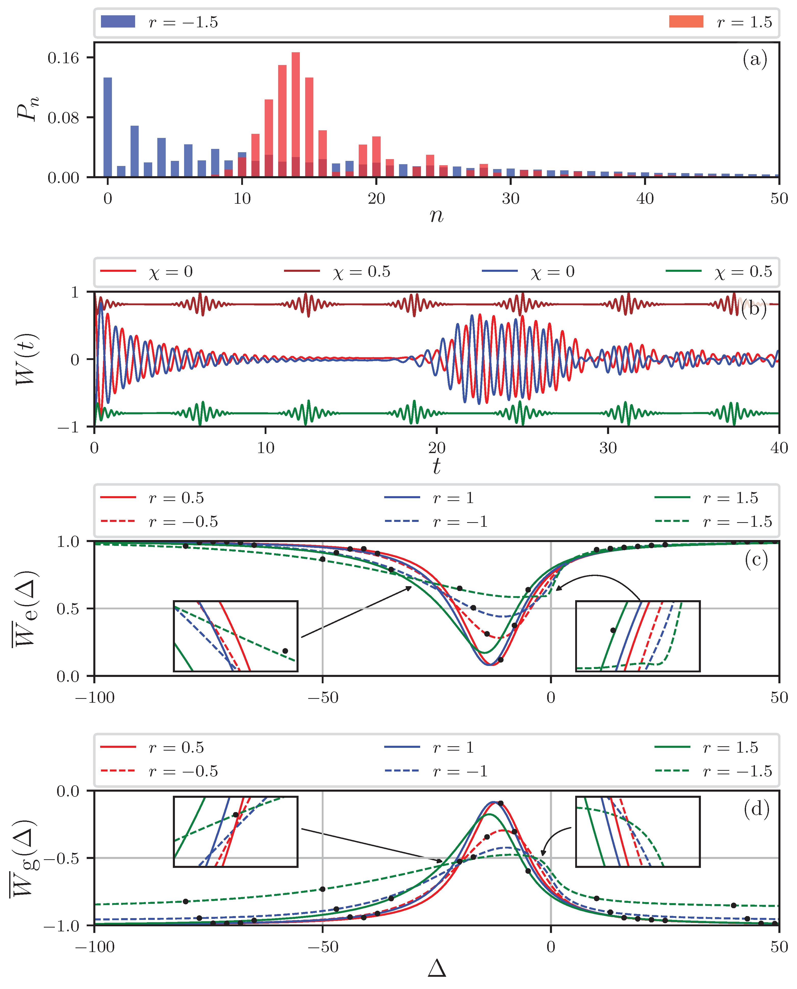
In Figure 2a, we show the photon number distribution of the initial squeezed coherent field for two different squeezing parameters, and $\alpha =3.5$. For $r=-1.5$, we obtain a wider distribution of photons, and we can also observe the difference between even and odd contributions. When $r=1.5$, additional smaller contributions can be observed accompanying the main contribution; these additional peaks will be responsible for the resonant revivals in atomic inversion [3].

Figure 2. (a) Photon number distribution for a squeezed coherent state with $\alpha =3.5$, and two values of r, −1.5 and 1.5. (b) Atomic inversion for $\chi =0.0$ (red line for the atom initially in the excited state and blue line for the atom initially in the ground states), and $\chi =0.5$ (brown line for the atom initially in the excited state and green line for the atom initially in the ground states), with $\alpha =3.5$, $r=1.5$, $\Delta =1$, and $g=1$. (c) Average atomic inversion as function of $\Delta$ for $\chi =0.5$, with the atom initially in the excited state and the field in a squeezed coherent state with $\alpha =3.5$ and six different values of r; again $g=1$. (d) In this case, the situation is the same as in (c), but preparing the atom in the ground state. In (c,d), the solid and dashed lines correspond to the analytical results, while the dots correspond to the numerical solution of the Schrödinger equation using QuTiP [30] and applied to (14). All the sums were evaluated with two hundred terms, which is more than enough given the behavior of the terms in the sums.

In Figure 2b, we present the atomic inversion $W\left(t\right)$, given by Equation (11), for an atom with $\Delta =g=1$, initially in the excited or ground state, and a field initially in a squeezed state. When $\chi =0$ (represented by red and blue lines for the excited and ground states, respectively), we observe an increase in the collapse time and the appearance of resonant revivals in the atomic inversion. However, considering the non-resonant nearby levels with $\chi =0.5$ (represented by brown and green lines for the excited and ground states, respectively), the atomic inversion approaches its initial value on average in the same manner as a coherent state; this is because levels outside of resonance affect the effectiveness of the field in driving transitions out of the initial state [4]. Furthermore, we note that the time for the first resurgence to appear shortens with increasing values of $\chi$, and the oscillations become more pronounced with increasing values of r, for both initial states of the atom. It is worth noting that for negative values of r, the atomic inversion exhibits irregular behavior with poorly defined rebirths; this behavior resembles the response of a thermal state to the field [22].

In Figure 2c, we plot the lineshapes when initially the atom is in its excited state and the field is in a squeezed coherent state, for different values of the squeezing parameter r; we use $\chi =0.5$, a value that falls within the validity range of the assumed approximation for the Hamiltonian (1) [15], and we set $g=1$. We can observe that for values of $\Delta >0$, i.e., when the frequency of the atom is higher than that of the field, the lineshapes rapidly decay towards the initial state of the atom, i.e., there are no transitions between the two levels, regardless of the value of the parameter r. On the other hand, for values of $\Delta <0$, we notice that as we increase the negative values of r in ascending order, the lineshapes become distorted and approach the initial state of the atom more rapidly, due to the widening of the probability distribution as the values of r decrease, as shown in Figure 2a. When we increase positive values of r, we observe that for small values of r, the lineshapes increase in depth until they reach a minimum point at $r=0.758$, corresponding to a depth of $0.9304$ (obtained numerically), and then begin to decrease in depth, maintaining an almost symmetrical shape with respect to their lowest point. However, as we further increase the value of r, the lineshapes become increasingly distorted and lose their symmetry.

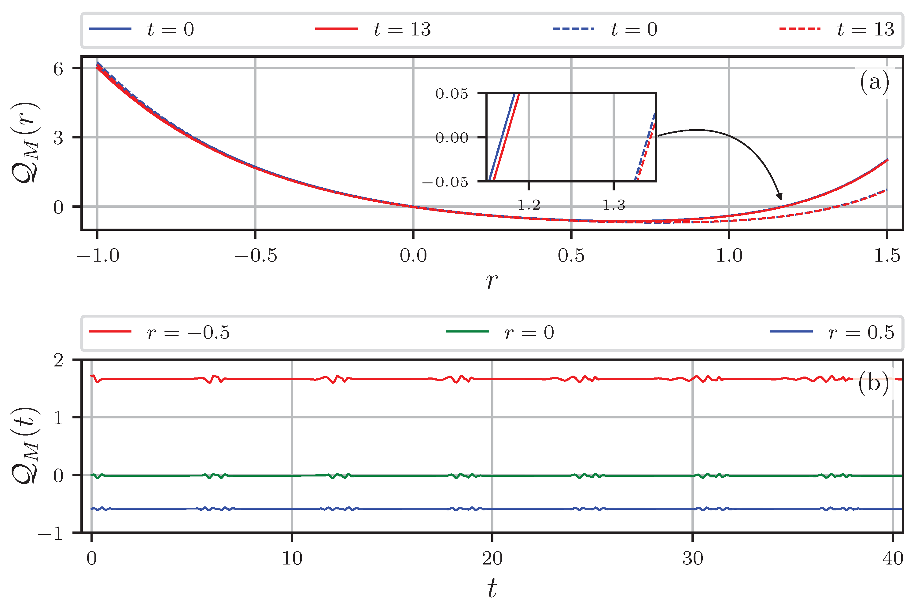
In order to achieve a deeper understanding of this behavior, we have plot the Mandel parameter ${\mathcal{Q}}_M$ in Figure 3. This parameter (not to be confused with the Husimi function Q) provides information about whether the photon distribution in the light state is sub-Poissonian (${\mathcal{Q}}_M<0$), Poissonian (${\mathcal{Q}}_M=0$), or super-Poissonian (${\mathcal{Q}}_M>0$). In Figure 3a, the continuous lines illustrate how the field undergoes a transition from super-Poissonian statistics ($r<0$) to sub-Poissonian statistics ($0<r<1.17$), and a return to super-Poissonian statistics ($r>1.17$), with parameter values $\alpha =3.5$, $\Delta =g=1$, and $\chi =0.5$. Furthermore, using dashed lines, we present the Mandel parameter ${\mathcal{Q}}_M$ for values of $\alpha =5$, $\Delta =0$, and $g=1$, as analyzed in [4]. This analysis exclusively considers the Jaynes–Cummings model in resonance, which exhibits transitions from super-Poissonian statistics ($r<0$) to sub-Poissonian statistics ($0<r<1.34$), followed by a return to super-Poissonian statistics ($r>1.34$). In Figure 3b, we also depict the behavior of the Mandel parameter ${\mathcal{Q}}_M$ as a function of time t for different values of r. This conduct is very different from the case of an initial field in a coherent state, where an increase in the average number of photons causes the lineshapes to widen and shift, while maintaining their symmetry with respect to the lowest point, as shown in [12].

Figure 3. The Mandel parameter ${\mathcal{Q}}_M$ is plotted as a function of (a) ${\mathcal{Q}}_M\left(r\right)$ for $t=0$ and $t=13$, and (b) ${\mathcal{Q}}_M\left(t\right)$ for various values of r. The parameter values employed are $\alpha =3.5$, $\Delta =g=1$, and $\chi =0.5$.

On the other hand, in Figure 2d, corresponding to the initial condition of the atom in the ground state, and for the same parameter values as in the previous case, it is important to note that the lineshapes are not a mirror image of the case where the atom is in the excited state, due to the presence of an additional excitation between the ground and excited states, as assumed in (4). All the graphics of (11), (13), (17), and (18) shown in Figure 2 (and subsequently, in Figures 6 and 7) were calculated with two hundred terms in the sums, which is more than enough given the structure of the terms and the behavior of $P_n$ with n. The numerical results were obtained by solving the Schrödinger equation using Python QuTiP 5.0.0 [30] tool and a Hilbert space dimension of two hundred.

4. Superposition of Squeezed Coherent States

In the previous section, it was shown that the lineshapes are very sensitive to the sign of the squeezing parameter r. In this section, we look at the lineshapes produced by a superposition of squeezed coherent states of the form

$$|{\psi }_{\pm }⟩=\frac{1}{{\mathcal{N}}_{\pm }}(|\alpha ,r⟩\pm |\alpha ,-r⟩),$$

(22)

where ${\mathcal{N}}_{\pm }=\sqrt{2[1\pm 1/\sqrt{cosh\left(2r\right)}]}$ is the normalization constant.

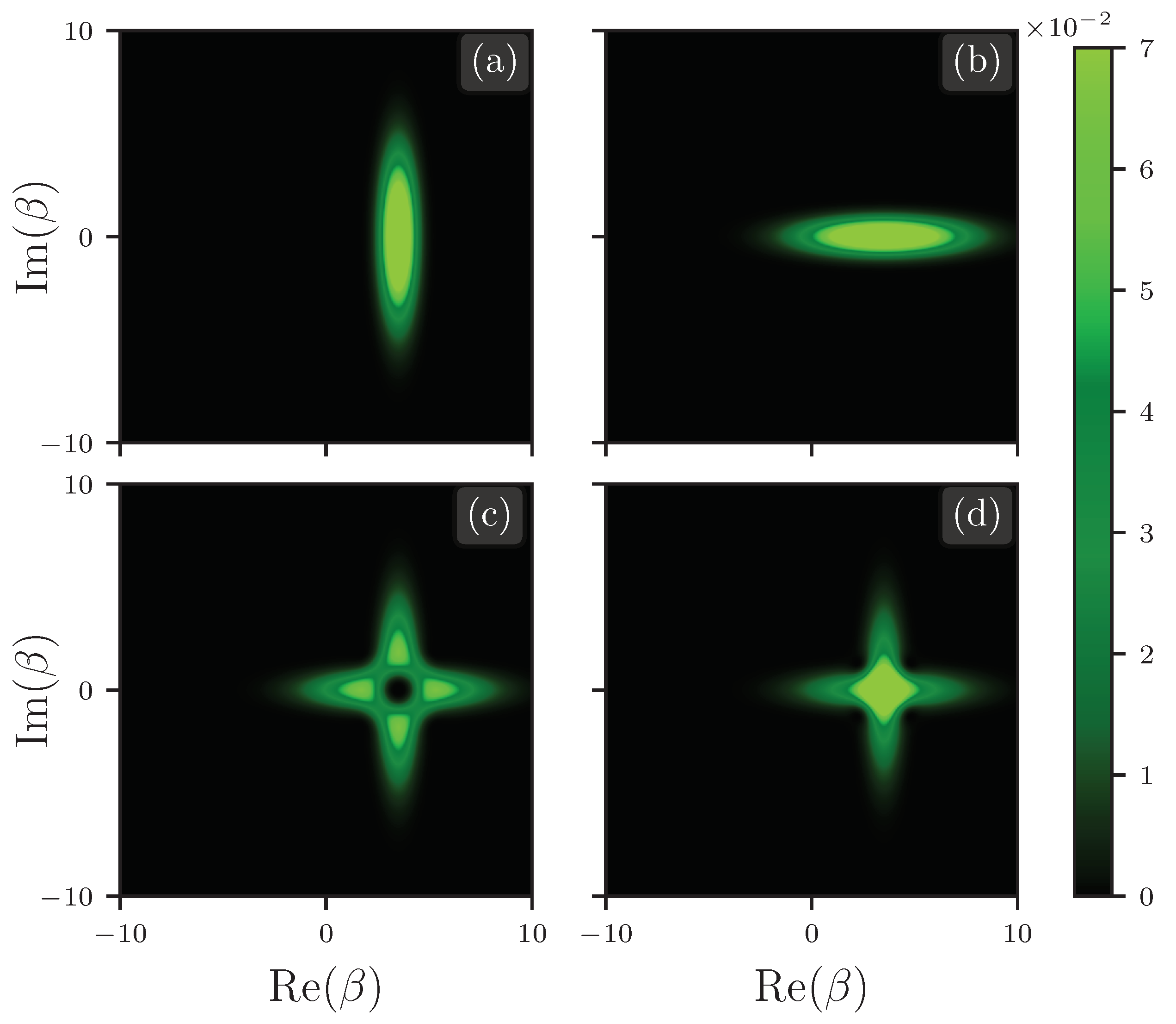
One way to visualize the behavior of quantum systems in phase space is through the Husimi Q-function. This function, also known as the quasiprobability distribution, was introduced by Kôdi Husimi in 1940 [31] and is commonly expressed as the expected value of the density operator [23],

$$Q\left(\beta \right)=\frac{1}{\pi }⟨\beta |\widehat{\rho }|\beta ⟩.$$

(23)

Based on the results obtained in Appendix A, we plot the Husimi Q-function for the squeezed coherent states (19) and for a superposition of the form (22) with $\alpha =3.5$. In Figure 4a, we can observe that, for positive values of r, the squeezing occurs in the real part of $\beta$, i.e., the uncertainty increases in the real part of $\beta$ and decreases in the imaginary part. On the other hand, for a negative squeezing parameter $r=-1.5$, in Figure 4b, the squeezing occurs in the imaginary part of $\beta$, which implies that the uncertainty increases in the imaginary part and decreases in the real part. In Figure 4c, corresponding to a negative superposition, we can observe that there is squeezing in both directions, except in the center. Finally, in Figure 4d, corresponding to a positive superposition, we can observe from the heat map that there is a maximum squeezing only at the center.

Figure 4. Husimi Q-function for the squeezed coherent states, with (a) $r=1.5$ and (b) $r=-1.5$. In addition, the Husimi Q function is presented for a superposition of squeezed coherent states of the form (22) with $r=1.5$. Figure (c) shows a negative superposition, and Figure (d) represents a positive superposition. In all cases, the amplitude used is $\alpha =3.5$.

Furthermore, the probability of finding n photons in a field defined by the state vector (22) is

$$P_n^{(\pm )}=\frac{1}{{\mathcal{N}}_{\pm }^2}{\left|⟨n|\alpha ,r⟩\pm ⟨n|\alpha ,-r⟩\right|}^2.$$

(24)

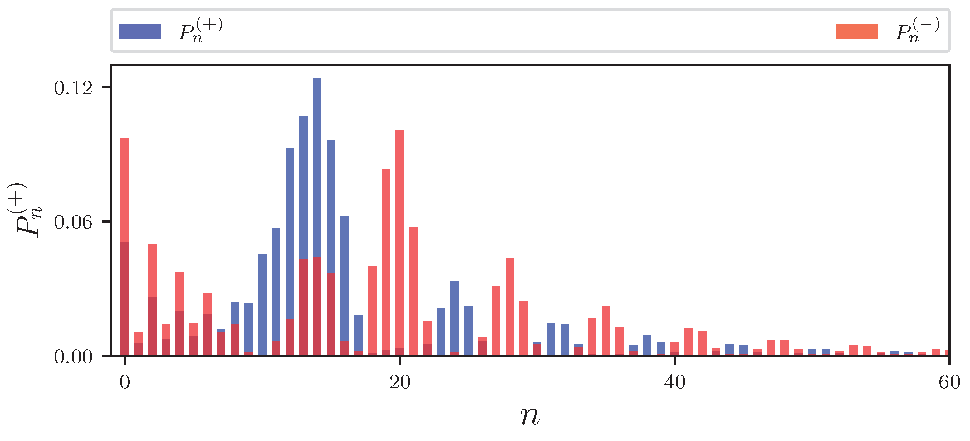
In Figure 5, we show the photon number distribution for a squeezed coherent state superposition, (22), with $r=1.5$ and $\alpha =3.5$. In the superposition $|{\psi }_{+}⟩$, we observe a photon number distribution $P_n^{(+)}$ that resembles that of a squeezed coherent state, with small contributions accompanying the main distribution; however, now $P_n^{(+)}$ also presents contributions before the main contribution. On the other hand, the photon number distribution $P_n^{(-)}$ for the superposition $|{\psi }_{-}⟩$ is notably different from that of $|{\psi }_{+}⟩$, since $P_n^{(-)}$ presents more than one main contribution, as well as a broader distribution.

Figure 5. The probability distribution of photons for a superposition of squeezed coherent states $P_n^{(\pm )}$, for $\alpha =3.5$ and $r=1.5$.

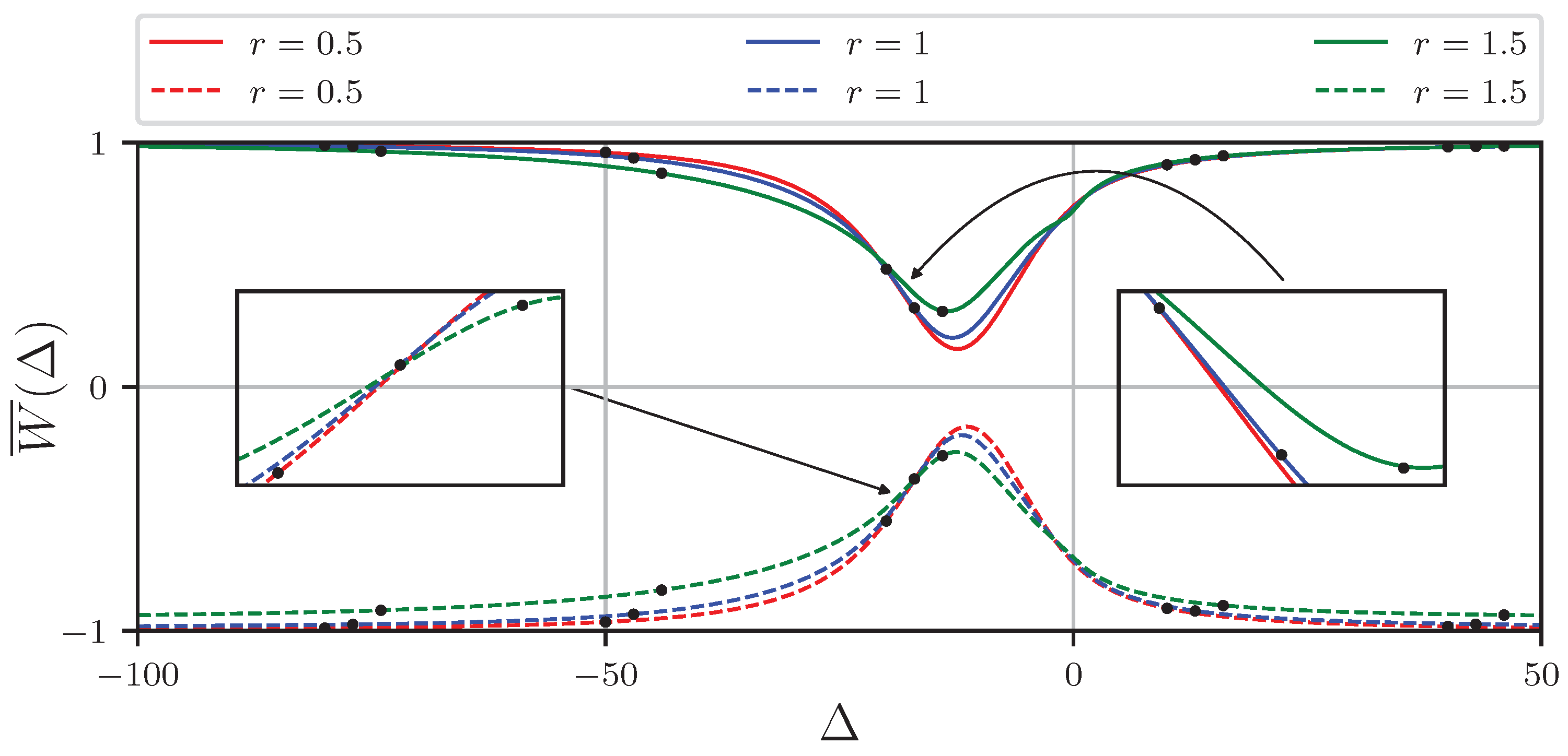
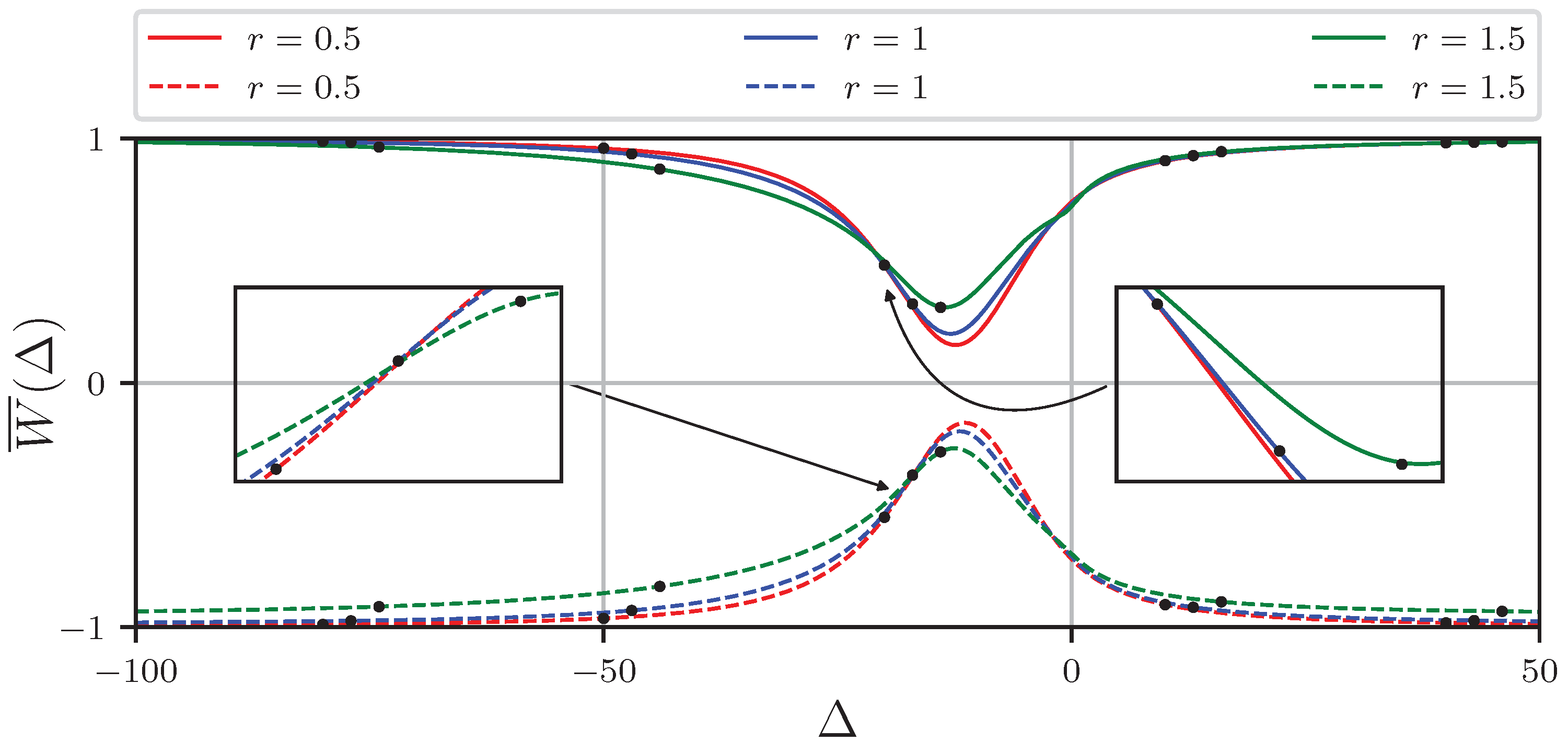
5. Results and Discussion

Figure 6 illustrates the lineshapes associated with a superposition of squeezed coherent states, denoted as $|{\psi }_{+}⟩$, under various initial conditions for the atom and different values of the squeezing parameter, r. These results are depicted with the following parameter settings: $\chi =0.5$, $g=1$, and $\alpha =3.5$. When the atom is initially in the excited state (solid lines), the lineshapes decay rapidly towards the atom’s initial state for positive detunings ($\Delta >0$), indicating negligible transitions between the two atomic levels, irrespective of the value of r. Conversely, for negative detunings ($\Delta <0$), the lineshapes for the superposition state $|{\psi }_{+}⟩$ exhibit behavior akin to a squeezed coherent state with $r>0$, owing to similarities in their photon distributions (see Figure 2c). Specifically, the lineshapes deepen until reaching a minimum at $r=0.308$, corresponding to a depth of $0.8478$ (numerically determined), after which they begin to shallow. However, these lineshapes exhibit less depth and distort more rapidly with increasing r compared to a squeezed coherent state. Furthermore, the symmetry around the minimum point is less pronounced compared to the case of a single squeezed coherent state.

Figure 6. Average atomic inversion $\overline{W}(\Delta )$ for the atom initially in the excited state (solid lines) and in the ground state (dashed lines), and the field in a superposition of squeezed coherent states $P_n^{(+)}$, for $\chi =0.5$, $g=1$, $\alpha =3.5$, and different values of r. The solid and dashed lines correspond to the analytical result, while the dots correspond to the numerical results.

Similarly, when the atom is initially in the ground state (dashed lines), the lineshapes resemble those of a squeezed coherent state with $r>0$ (see Figure 2d). However, it is crucial to note that the lineshapes are not mirror images of the case where the atom is initially in the excited state. This distinction becomes more apparent for sufficiently large values of r.

We now turn our attention to the average atomic inversion corresponding to a superposition of squeezed coherent states denoted as $|{\psi }_{-}⟩$, under the same atomic conditions as in the previous scenario (Figure 6) and with identical parameter values. As depicted in Figure 7, when the atom is initially in the excited state (solid lines) and $\Delta >0$, the curves decay rapidly, similarly to $|{\psi }_{+}⟩$. However, for $\Delta <0$, they exhibit a distinct behavior characterized by a slower decay and rapid distortion with increasing r, accompanied by the emergence of multiple minima, which proliferate with higher values of $\chi$. It is noteworthy that the Hamiltonian (1) restricts $\chi$ to values not exceeding 1. Importantly, the symmetry around the minimum point is lost in this scenario.

Figure 7. Average atomic inversion $\overline{W}(\Delta )$ for the atom initially in the excited state (solid lines) and in the ground state (dashed lines), and the field in a superposition of squeezed coherent states $P_n^{(-)}$, for $\chi =0.5$, $g=1$, $\alpha =3.5$, and different values of r. The solid and dashed lines correspond to the analytical result, while the dots correspond to the numerical results.

Finally, when the atom is initially in the ground state (dashed lines), the curves display a more pronounced disparity compared to all previous cases. This discrepancy arises from the super-Poissonian shape of its probability distribution and the presence of an additional excitation between the ground and excited states, as previously discussed.

Now, we analyze the average atomic inversion corresponding to a superposition of squeezed coherent states $|{\psi }_{-}⟩$, with the same atomic conditions as in the previous case (Figure 6) and for the same parameter values. We observe in Figure 7 that when the atom is initially in the excited state (solid lines) for values of $\Delta >0$, the curves decay rapidly in a similar manner to $|{\psi }_{+}⟩$; however, for values of $\Delta <0$, they exhibit a very different behavior. In this case, the curves decay more slowly but distort rapidly as the values of r increase, and they also display multiple minima. In fact, the number of minima increases as the parameter $\chi$ value increases. However, as mentioned before, the Hamiltonian (1) is restricted to values of $\chi$ that do not exceed 1. It is important to note that, in this case, the symmetry with respect to the minimum point no longer exists. Finally, when the atom is initially in the ground state (dashed lines), the curves exhibit a much more noticeable difference than in all previous cases. This is due to the super-Poissonian shape of its probability distribution (see Figure 5) and the presence of an additional excitation between the ground and excited states, as mentioned before.

6. Conclusions

In summary, our investigation has shed light on the remarkable sensitivity of micromaser lineshapes to the squeezing parameter r. For small positive values of r, characterized by a sub-Poissonian photon distribution, the lineshapes of squeezed coherent states exhibit almost symmetric profiles around their minimum points. However, as r takes on negative values, leading to a super-Poissonian photon distribution, the lineshapes undergo rapid distortion, resulting in broadened and asymmetric profiles. This behavior stems from the presence of two distinct photon distribution types in squeezed states with negative r: an oscillatory distribution and a coherent-like distribution, which imprint on opposite sides of the lineshape.

Furthermore, our exploration extends to the behavior of superpositions of squeezed coherent states with equal amplitude. When the superposition’s sign is positive, the lineshapes resemble those of a squeezed coherent state with $r>0$, albeit with a more rapid distortion. Conversely, when the sign of the superposition is negative, the lineshapes distort even more rapidly with increasing r, exhibiting multiple minima. These findings underscore the critical importance of considering the sign of the squeezing parameter in the analysis of micromaser lineshape dynamics.

Our study contributes to a deeper understanding of the intricate interplay between squeezing parameters and micromaser lineshapes, offering valuable insights for the design and optimization of micromaser systems. Future investigations could delve into exploring the effects of additional parameters or extend the analysis to more complex quantum systems, paving the way for enhanced control and manipulation of quantum states in various applications.