Article

Spatial Fluctuations of Optical Turbulence Strength in a Laboratory Turbulence Simulator

1
Key Laboratory of Atmospheric Optics, Anhui Institute of Optics and Fine Mechanics, Hefei Institutes of Physical Science, Chinese Academy of Sciences, Hefei 230031, China
2
Science Island Branch, University of Science and Technology of China, Hefei 230026, China
*
Author to whom correspondence should be addressed.
Photonics 2024, 11(3), 229; https://doi.org/10.3390/photonics11030229
Submission received: 27 January 2024 / Revised: 28 February 2024 / Accepted: 28 February 2024 / Published: 1 March 2024

Abstract

:
Controlled turbulence simulators in the laboratory have been extensively employed to investigate turbulence effects on light propagation in the atmosphere, driven by some advanced optical engineering such as remote sensing, energy-delivery systems, and free-space optical communication systems. Many studies have achieved rich results on the optical turbulence intensity, scintillation index, and power spectral density characteristics of the light propagation path in the center of a turbulence simulator, but a comprehensive analysis of the optical turbulence characteristics for different spatial locations is still lacking. We simulate turbulence with air as the medium in a classical convective Rayleigh–Bénard turbulence simulator through high-resolution computational fluid dynamics methods, the three-dimensional refractive index distribution is obtained, and the optical properties are analyzed comprehensively. It is found that the hot and cold plumes and the large-scale circulation strongly influence the inhomogeneity of C n 2 in the turbulence tank, making it weak in the middle and strong near the boundary. The refractive index power spectral density at different heights is centrally symmetric, with the slope gradually deviating from the −5/3 scaling power with increasing distance from the central region. Under the log-log plot, the variation of the refractive index variance with height exhibits a three-segmented feature, showing in order: a stable region, a logarithmic profile, and a power-law profile, in the region close to the boundary. These results will contribute to the construction of a suitable turbulence simulator for optical engineering applications.

1. Introduction

Optical turbulence arises predominantly from the spatial and temporal fluctuations of density within the Earth’s atmosphere; these fluctuations give rise to an inhomogeneous refractive index distribution, resulting in intensity fluctuation, and phase distortion [1,2]. Consequently, the propagation of optical signals is significantly affected [3]. This presents substantial challenges across multiple domains of optical engineering such as remote sensing, energy-delivery systems [4], and free-space optical communication systems [5]. Understanding and mitigating the impact of optical turbulence are essential for advancing and optimizing optical technologies. A laboratory turbulence simulation facility for optical turbulence provides a controlled and reproducible environment for a detailed study of turbulence phenomena.
Since temperature is the main factor affecting the air refractive index [6], laboratory turbulence simulation devices are often designed to adjust the turbulence strength by controlling the temperature. Rayleigh–Bénard (RB) convection is a widely investigated nonlinear system used to design laboratory turbulence simulation devices [6,7,8,9,10,11,12,13]. These simulators use air or water in an enclosed space to generate a buoyancy-driven flow by heating the bottom and cooling the top, establishing a thermal gradient where the heated fluid rises, and the cooled fluid sinks, forming convective cells, enabling controlled generation, observation, and measurement of turbulence under well-defined experimental conditions. The strength of turbulence can be changed by adjusting the temperature difference between the bottom and top [6,12,14,15,16,17].
The characterization of RB convection provides essential insights to mitigate the effects of optical turbulence on laser beams in random media [18]. This is why convective RB turbulence simulators have received significant attention [10,11,17,18,19,20]. Many experiments have focused on analyzing the light intensity and phase fluctuations of convective RB turbulence simulators with water and air as media through the path-integrated received light fields [14,18,20]. Many other simulation works have provided a wealthy study of RB convection with water as media through a combination of computational fluid dynamics (CFD) and wave-optical simulations [6,12,15]. Although the RB turbulence with water as the medium can easily achieve large turbulence strengths, it is more difficult to obtain turbulence with a homogeneous and wide inertia region because the thermal conductivity of water is much larger than that of air. However, there is no comprehensive analysis of simulations using air as a medium to study the three-dimensional turbulence strength inside a turbulence simulator and the scaling power analysis of non-Kolmogorov turbulence at different heights. Therefore, it is necessary to simulate and analyze the RB turbulence simulator with air as the medium and verify whether the simulated turbulence conforms to the characteristics of atmospheric turbulence.
In previous turbulence simulators, the turbulence is usually assumed to satisfy the local homogeneity and isotropy assumptions. However, based on the characteristics of the large-scale circulation of RB turbulence, it is known that the spatial distribution of this turbulence simulator is inhomogeneous. It is highly necessary to study the turbulence characteristics at different spatial locations within the turbulence simulator, and it is essential to clarify the influence of the upper and lower boundaries on the turbulence power spectrum density, the variation of the scaling power of the non-Kolmogorov turbulence as well as the profile of the turbulence strength as a function of height.
This study focuses on the structural characteristics of optical turbulence in a laboratory turbulence simulation facility. We conducted high-resolution, fluid dynamics simulations of the flow field within the turbulence simulator using large-eddy simulation (LES). By utilizing the obtained information on the temperature field, pressure field, and density field, we calculated a three-dimensional refractive index field. Subsequently, an analysis of the optical turbulence structure was conducted based on the three-dimensional refractive index field. Furthermore, we analyzed the second-order statistical properties related to the anisotropic fluctuation of the refractive index.

2. Theoretical Foundation of RB Convection and Simulation

2.1. Governing Parameters of RB Convection

The incompressible Navier–Stokes equation with Boussinesq approximation to account for RB convection is a buoyancy-driven turbulence system. The dimensionless governing equations of RB convection are as follows [21,22,23]
u t + u u = p + Pr Ra 2 u + T e y
T t + u T = 1 Ra Pr 2 T
u = 0
where u = ( u , v , w ) is the velocity field, and T = T i T 0 is the fluctuations of temperature field and p is the pressure field, T i is the temperature at a point in space, T 0 is the average temperature and p is the pressure field. e y represents the gravity vector in the vertical direction, with x r e f = H , u r e f = g α Δ T H as the velocity scale, T r e f = Δ T = T h T c , T h is the temperature of the heating plate, T c is the temperature of the cooling plate.
The governing parameters of RB convection are the Rayleigh number Ra, which is the dimensionless temperature difference between the bottom and top plates, Prandtl number Pr, which is the ratio between kinematic viscosity ν and thermal diffusivity κ , and the aspect ratio Γ , which represents the geometry of the convective system [23,24].
For which
R a = g α Δ T H 3 / ( ν κ )
Pr = v / κ
Γ = W / H
where the g stands for the acceleration due to gravity, α is the thermal expansion coefficient, and H is the height between the top and bottom plates, W, is the horizontal width of the convective system.
The geometry of the turbulence simulator is generally constant so the aspect ratio is fixed. And the Pr is 0.7 for atmospheric flows [21,25,26]. Therefore, the convective turbulence strength within the RB turbulence tank can be changed by controlling the temperature difference between the top and bottom plates. As the temperature difference increases, the flow field will enter a turbulent state, and the critical Ra is generally considered to be around 1.9 × 10 8 [27,28]. For air, the maximum temperature under the Oberbeck–Boussinesq (OB) approximation is 28.6 K [27]. In our study, Ra ranges from 4.7 × 10 8 to 1.9 × 10 9 , corresponding to Δ T running from 5 K to 20 K. The total heat transfer is expressed by the Nusselt number Nu, which is defined as
N u = Q H κ Δ T
where Q is heat flux. Nu indicates the convective heat transfer efficiency of the system.

2.2. LES of the RB Turbulence Simulator

Numerical simulation is an important tool for the study of turbulent thermal convection. Direct numerical simulation (DNS) is an effective tool for analyzing RB turbulence tank. It is used by directly solving the Navier–Stokes equations without modeling and simplifying the turbulence. However, it requires significant computational resources at the same resolution [29]. Reynolds-averaged Navier–Stokes (RANS) models, while useful in predicting turbulence parameters, cannot resolve the details of the smaller flow features and associated eddies [6]. In LES, the flow explicitly resolves the large-scale eddies, while the smaller scales below the grid-size are modeled [30]. LES can obtain a more detailed structure of the flow field than RANS, and uses less computational resources than DNS, since DNS requires a large amount of computation at large Ra numbers, and since we need to compute for several temperature differences. On balance, LES is the preferred simulation method for high Ra conditions, and in our analysis we focus on the structural properties of the optical turbulence.
Geometry and meshes: In our study, LES was performed in a closed turbulence tank using air as the working fluid with dimensions of 1   m × 1   m × 1.2   m , heating at the bottom, cooling at the top. In order to facilitate the conversion to optical parameters and statistical analysis, quadrilateral grid cells were chosen for meshing. We conducted the numerical simulations on high-performance computers with a grid resolution of 5 mm, which corresponds to 9.6 million grid points in a 1   m × 1   m × 1.2   m domain. The grid resolution of 5 mm was chosen based on the typical inner l 0 scale of optical turbulence, as discussed in Matt et. al. [6], to keep computational demands manageable.
Boundary conditions: All boundaries are designed with no-slip boundaries, with a constant temperature difference Δ T = T h T c between the top and bottom plates, and the side walls are thermally insulated [25].
u = 0 , T n = 0
Subgrid-scale (SGS) mode: In LES, spatial filtering allows small-scale motions to be modeled and large-scale motions associated with boundary conditions to be resolved directly. LES filtered equations can be expressed as
u j ¯ t + u j ¯ u j ¯ x j = p ¯ x i + Pr Ra u i ¯ x j 2 + T ¯ δ i 2 τ i j x j
T ¯ t + u j ¯ T ¯ = 1 Ra Pr 2 T ¯ x j 2 σ j x j
where u j ¯ is the filtered velocity, p ¯ is the filtered pressure, T ¯ is the filtered temperature. τ i j is the subgrid-scale (SGS) stress tensor, σ j is the SGS heat flux vector. And we approximate the effect of the under-resolved scales as
τ i j = u i u j ¯ u i ¯ u j ¯
σ j = u j T ¯ u j ¯ T ¯
The Smagorinsky–Lilly model was chosen as the subgrid-scale (SGS) model which uses an eddy viscosity formulation [6,29,31]
τ i j = 2 v T S i j ¯ + 1 3 τ k k δ i j
σ j = v T Pr T ¯ x j
where τ k k is the isotropic part of the SGS stresses, which is added to the filtered static pressure term. S i j ¯ can be expressed as
S i j ¯ = 1 2 u i ¯ x j + u j ¯ x i
where v T is the eddy viscosity, the Smagorinsky–Lilly model in ANSYS Fluent defines turbulent eddy viscosity as follows:
v t = ρ L s 2 S ¯
where S ¯ = 2 S i j ¯ S i j ¯ , and L s = min ( K d , C s Δ ) is the mixing length for subgrid scales, K = 0.41 is the von Karman constant, d is the distance to the closest wall, C s is the Smagorinsky constant, C s = 0.1 has been found to yield the best results for a wide range of flows, and Δ = V 1 / 3 is the local grid scale.
As in reference [6], considering that the frequency of most optical devices is mostly 100 fps, we choose a time step of Δ t = 0.01 s. We set the initial environment of the air with a temperature of 293.15 K. The detailed parameters are shown in Table 1.
We conducted parallel computing on high performance computers using multiple nodes, each with 128 cores, powered by two AMD 7702 processors per node, which took a few days to reach a steady state in turbulence at each temperature difference, and we simulated five temperature conditions, which took about 5 × 10 6 core hours. Figure 1a shows a schematic of an application setup for an optical turbulence simulator, Figure 1b shows the variation of Nusselt number with time for different temperature differences, and it can be seen that the Nusselt number is almost stabilized after 300 s, and the larger the temperature difference (Ra) the larger the Nusselt number. The Nusselt number is approximately proportional to the Rayleigh number to the 0.3 power. This is consistent with the power law of RB convection and proves that the simulation is performed correctly [32,33].

3. Characterization of the Flow Field in the RB Turbulence Simulator

The numerical simulations provide three-dimensional fields of temperature, density, and velocity, providing an overview of the overall circulation within the simulator. Figure 2 shows the instantaneous temperature field on the longitudinal section parallel to the z-axis of the turbulence tank at different moments under a temperature difference of 15 K. As can be seen from the Figure 2, the bottom heating surface forms a typical thermal plume, which continues to spread upwards as turbulence develops over time, causing the temperature inside the RB turbulence tank to rise. The buoyancy force causes the thermal plume to rise along one side of the wall and fall from the other side, forming a large-scale circulation. The size and quantity of the convective cells formed in the tank depend on the tank’s dimensions, particularly its height. In our specific case, with a tank of depth L y = 1   m and length L z = 1.2   m and the aspect ratio Γ = L z / L y = 1.2 , a large convection cell is formed in the fluid region as shown by the red dashed line in Figure 2d.
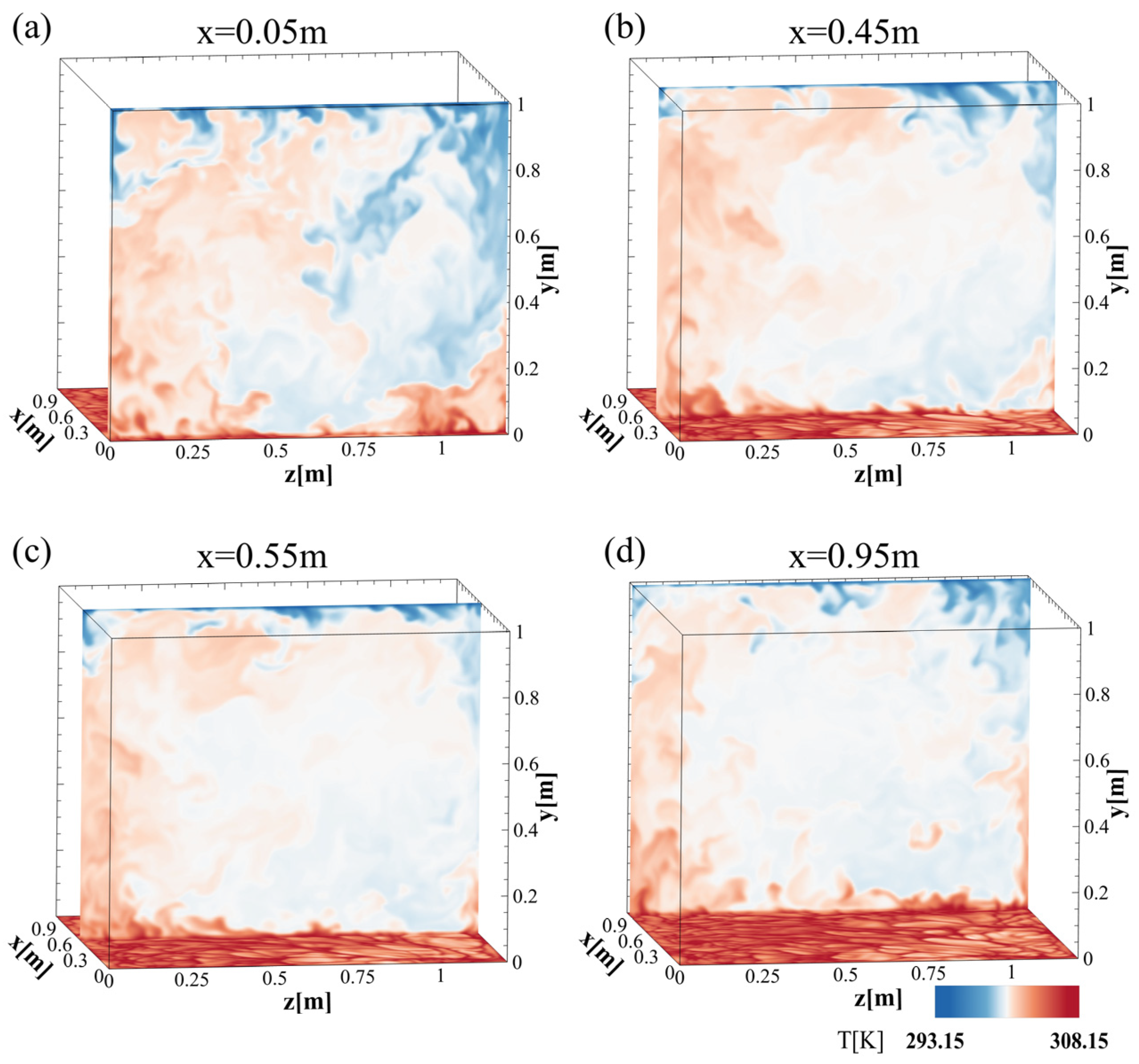
Figure 3 shows the instantaneous temperature field at Δ T = 15   K , t = 455 s, for different yz-planes. Figure 3a,d show longitudinal sections near the side walls, while Figure 3b,c show longitudinal sections on both sides of the center. At various positions in the longitudinal sections, classical cold and hot plumes near the boundaries, along with large-scale circulation, are observed. Figure 4 shows the instantaneous temperature field distribution on a cross-section of the xy-plane, perpendicular to the z-axis. Figure 4a,d illustrate the temperature distribution near the boundaries, showing cross-sections of hot plumes carrying heat upward and cold plumes moving downward under buoyancy within the large-scale circulation. Figure 4b,c represent steady regions within the large-scale circulation field.
Figure 5 shows the transient temperature field in the x-z plane at different locations for a temperature difference of 15 K. From the temperature field, it is clear that there is a temperature gradient in the perpendicular direction. In the turbulence tank, cold and hot plumes originate at the temperature boundaries of the top and bottom plates, separate, and enter the central region under the influence of buoyancy and the plume motion leads to the formation of a large-scale convective cell. The roll-like structure of the convective cell means that a central region exists along the center of the tank.

4. The Refractive Index Structure Constant C n 2

The key parameter for the conversion of hydrodynamic turbulence into optical turbulence is the refractive index. For dry air the refractive index of visible wavelengths is a function of temperature T (K), and atmospheric pressure P (kPa) [1],
n = 1 + 7.86 × 10 4   P / T
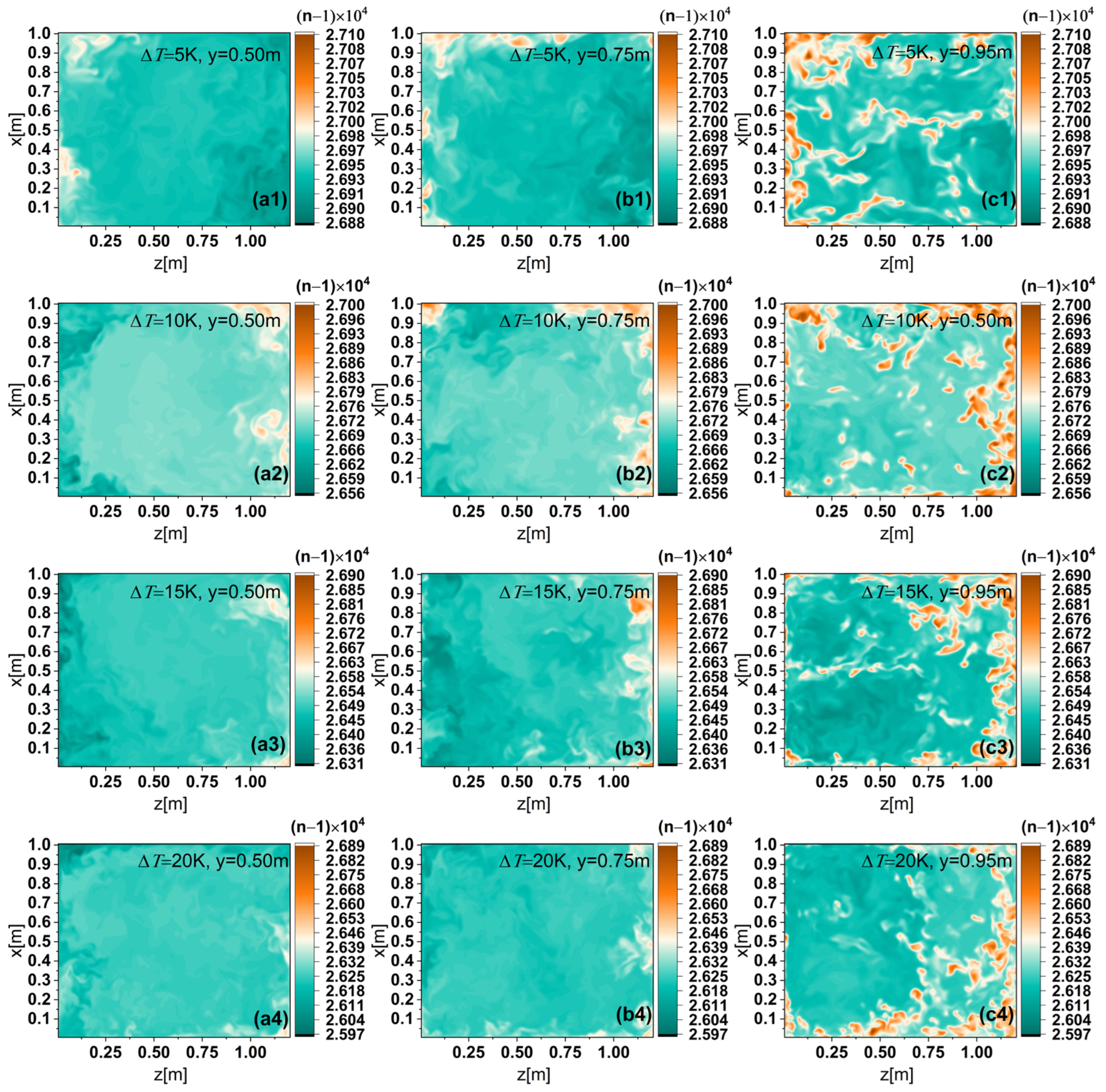
In the RB turbulence tank, temperature differences between the bottom and upper plates cause the refractive index field to fluctuate spatially. The refractive index can be obtained from Equation (17). Figure 6 shows the refractive index distribution in the xz-plane at different heights in the turbulence simulator for different temperature differences. Different columns of Figure 6 show the refractive index fluctuation field under different temperature difference, Δ T , conditions, which shows that the increase in temperature difference decreases the value of refractive index fluctuation. Figure 6a–c show the refractive index field at y = 0.5 m, y = 0.75 m, and y = 0.95 m locations in the horizontal cross-section, respectively, with the degree of fluctuation of the refractive index field increasing with height.
The inhomogeneous distribution of refractive index in three dimensions, resulting from temperature gradients, is often quantified using its second-order statistical properties such as the correlation function and structure function, which provide the scale of turbulence in space and the distribution of energy, respectively.
The structure function, associated with the random field, is defined by [3] as
D n ( r 1 , r 1 + r ) = n r 1 + r n r 1 2
where the brackets   denote an ensemble average.
In a homogeneous and isotropic random field, the structure-function can be simplified to a form that only depends on the scalar distance r = r . The refractive index structure function follows the form [3]:
D n ( r ) = C n 2 r 2 / 3 , ( l 0 r L 0 )
where the l 0 [m] is the inner scale, and L 0 is the outer scale. C n 2 is the refractive index structure constant (in units of m−2/3), which quantitatively represents the strength of optical turbulence.
As shown in Figure 7, C n 2 at different locations were obtained by calculating the refractive index structure function with a distance between the planes of 0.15 m, according to Equation (8). Each C n 2 was spatially averaged over ten transient neighboring data, and statistically temporally averaged over 500 frames of data. As can be seen from the figure, due to the aspect ratio of 1.2, only one convection cell exists. The convection cells’ roll-like structure suggests a core region along the center of the tank, the turbulence strength in the core area is significantly smaller than that in the boundary region. The strong boundary range of C n 2 between the upper and lower plates expands due to vertical temperature gradients, while the core region continuously diminishes. This indicates that the hot and cold plumes and the large-scale circulation strongly influence the inhomogeneity of C n 2 in the turbulence tank.
Figure 8 shows the C n 2 distribution at different locations in the horizontal direction, which indicates the C n 2 distribution near the lower boundary region, the center region, and the region near the upper boundary, respectively. It can be seen that the C n 2 in the horizontal direction is greatly affected by the large-scale circulation; in the boundary region of the large-scale circulation, the C n 2 exceeds 10 13 within the range of strong turbulence, while the C n 2 in the central region fluctuates in a larger range of 10 16 to 10 11 , and in the region close to the sidewall surface the C n 2 is larger, and in the center of the body the C n 2 is smaller.
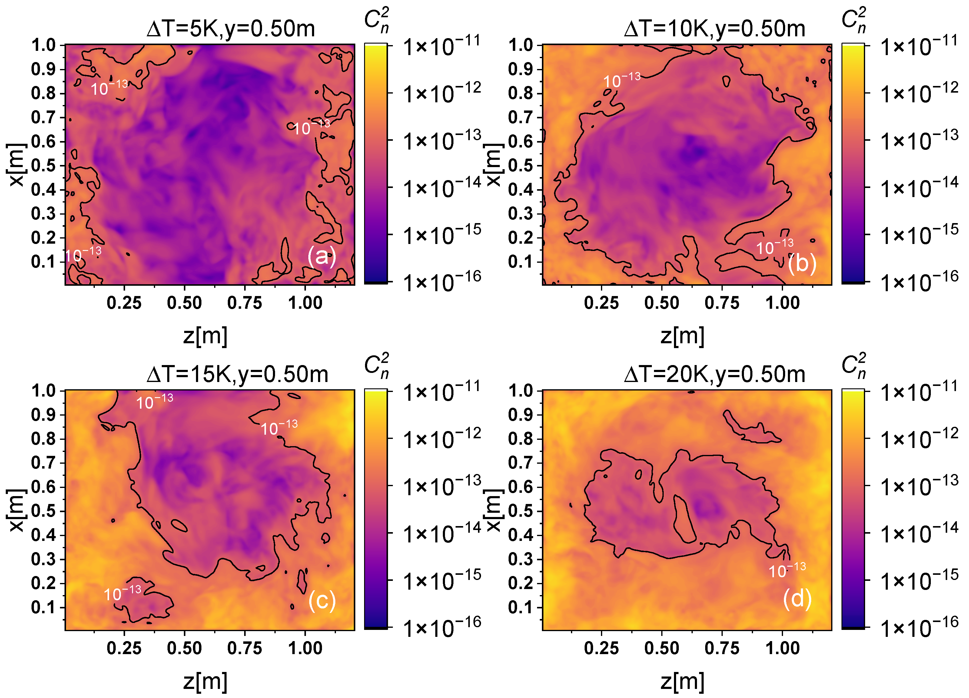
The turbulence simulator with the atmosphere as a medium usually uses insulating material that is not visible. The light path is usually set up only at the center, and the choice of the light aperture directly limits the maximum beam waist radius of the beam being tested. Therefore, it is crucial to understand the distribution of C n 2 horizontally at the middle height of the turbulence simulator to set up the light aperture appropriately. The C n 2 distribution in the xz-plane, which is parallel to the upper and lower plates at different temperatures, is shown in Figure 9. Figure 9a shows the C n 2 distribution between the upper and lower plates at 5 K. It can be seen that the turbulence intensity at this time varies considerably between the regions far away from the boundary and close to the boundary, with moderate turbulence in the central region and strong turbulence in the near boundary region. As the temperature difference increases, the C n 2 in center region is increasing and the percentage of strong turbulence in the turbulence simulator increases. This is due to the large refractive index fluctuations formed by the hot and cold plume across the horizontal cross-section, resulting in a higher strength of C n 2 in the near boundary region and a relatively weak C n 2 in the smooth region where the refractive index fluctuations are smaller. An increasing temperature gradient leads to strong refractive index fluctuations, thus the strong turbulence over a wider area of the horizontal cross-section. Meanwhile, the influence of the sidewall surface on C n 2 shows a different effect in the two orthogonal directions in the horizontal cross-sections, with the plume leading to a stronger C n 2 in the near-boundary region perpendicular to the long edge, while the C n 2 in the near-boundary region parallel to the long edge is relatively weaker.

5. Fried Parameter

The Fried parameter, also known as the atmospheric coherence length, r 0 , has been used in previous studies of turbulence simulators to quantify the intensity of turbulence over the entire propagation path. Our results show that r 0 varies spatially and is inhomogeneous at different positions in the RB turbulence simulator. Hence, we explore the profile of r 0 at various heights within the simulator.
Based on the relationship between the refractive index structure constant C n 2 and the atmospheric coherence length r 0 [34] is given by
r 0 = 0.423 k 2 0 Δ z C n 2 ( z ) d z 3 / 5
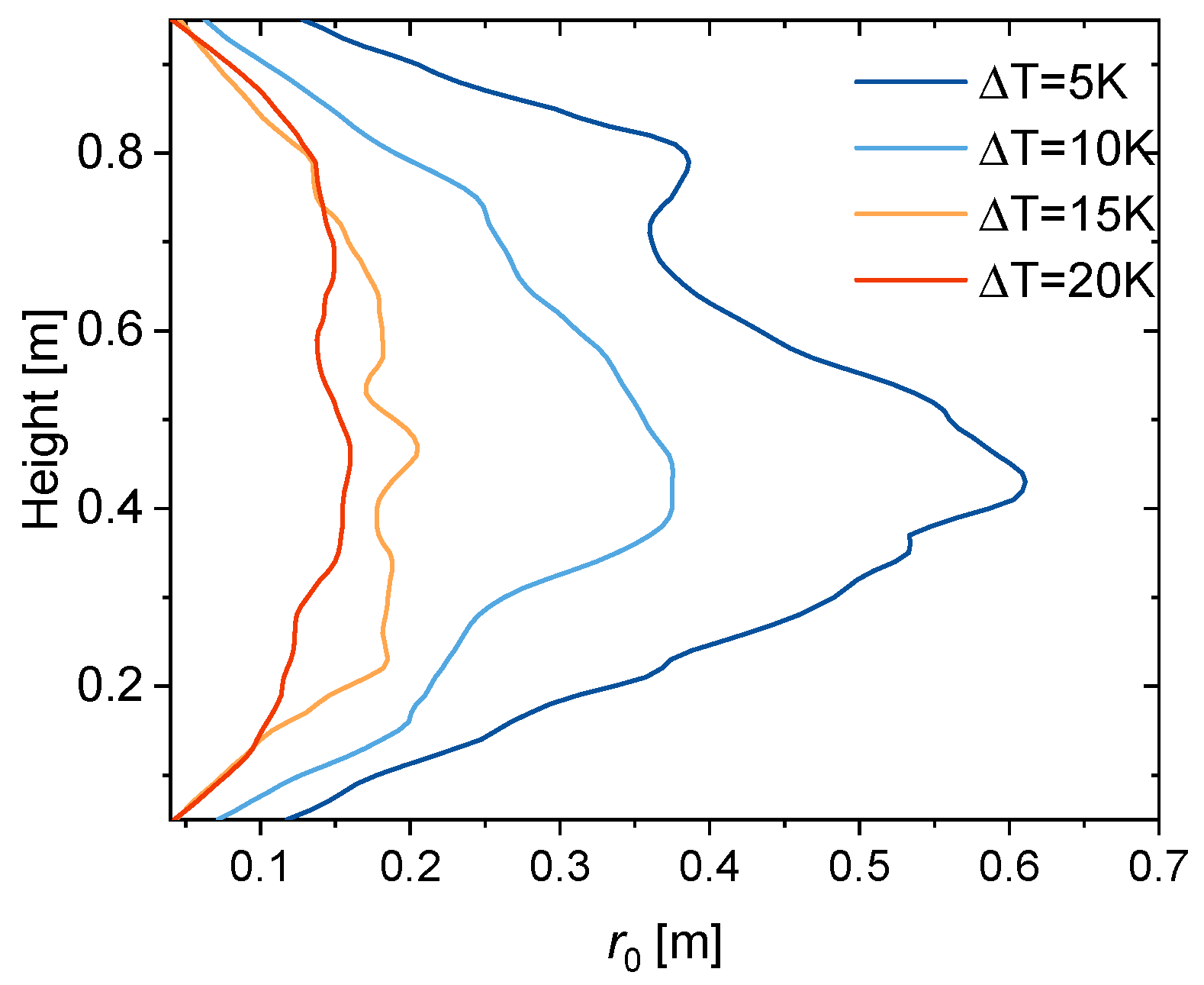
We calculated the values of r 0 at different heights. As shown in Figure 10, r 0 shows a trend of increasing and then decreasing with respect to the y-direction, and r 0 is maximum at the center. As the temperature difference gradually increases, the turbulent field energy keeps increasing and the velocity of the convective cell gradually increases, which leads to a gradual decrease of the r 0 value in the central region. This indicates that the turbulent decoherence effect on the propagating beam from the center region of the turbulence simulator is gradually increasing with the temperature difference.

6. One-Dimensional Refractive Index Power Spectral Density

Based on the 2/3 scaling power expression in Equation (19) of the refractive index structure function in the inertial subrange, the three-dimensional power spectral density (PSD) can be defined by [3]
Φ n ( K ) = 0.033 C n 2 K 11 / 3 f ( K l 0 )
where K is the spatial frequency in 1/m, and l 0 is the inner scale. For Kolmogorov refractive index PSD f ( K l 0 ) = 1 . Thus, the one-dimensional PSD of the refractive index fluctuations in the inertial subrange is given by
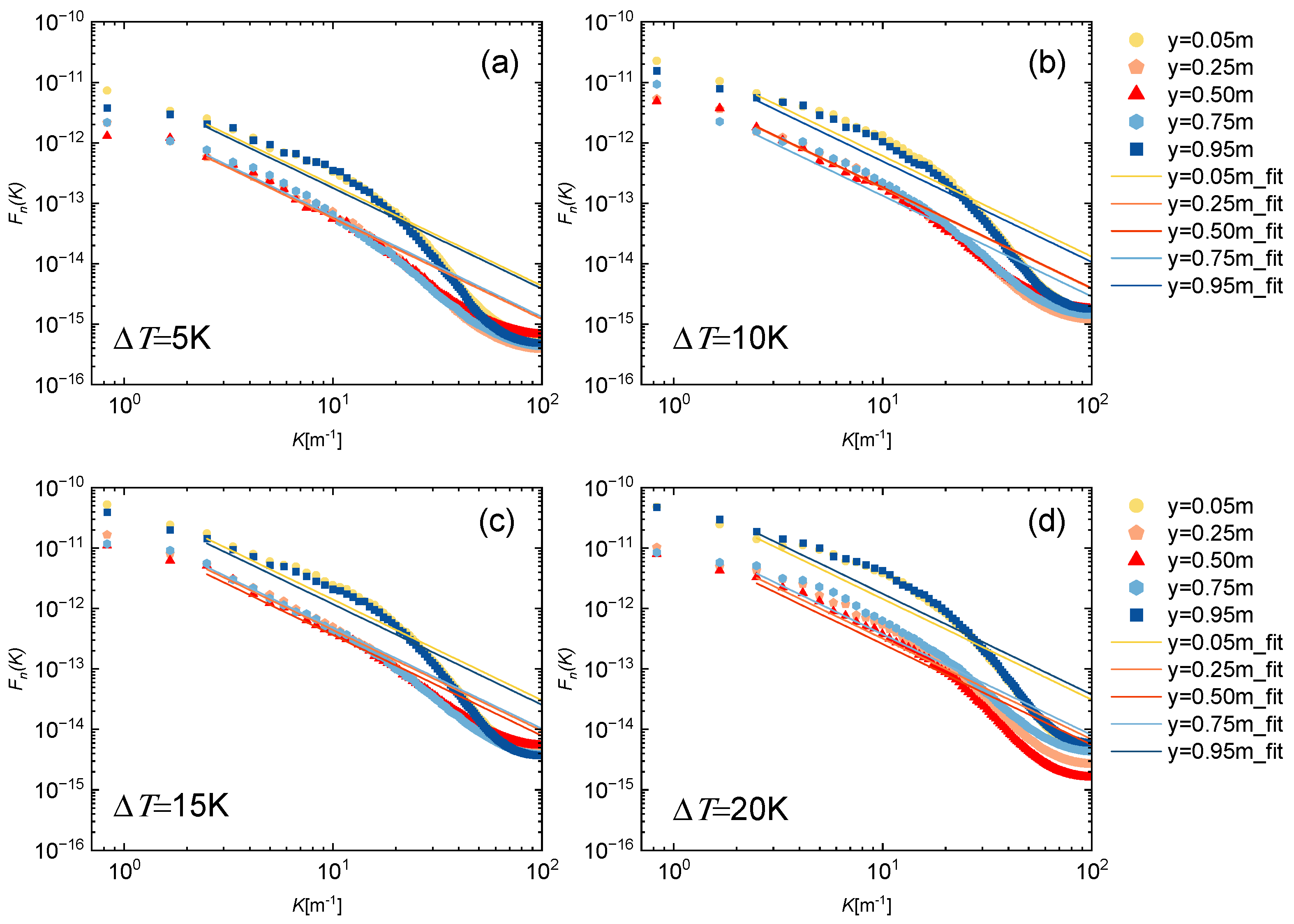
F n ( K ) C n 2 K 5 / 3
We studied PSDs at different heights in turbulence simulators to analyze the range of −5/3 scaling power. We make a periodogram estimation to compute the PSD of a random signal, which takes the square of the mode of N spatial random signals with a Fourier transform and divides it by N. We averaged the data over planes of the same height and counted 500 frames of data averaged over data intervals of 0.01 s. Figure 11 shows the variation of spatial PSD of refractive index under different temperature differences, and it can be found that the PSD at the heights of y = 0.95 m and y = 0.05 m almost overlap; meanwhile, the PSD at y = 0.25 m and y = 0.75 m are close to the data at y = 0.5 m. This indicates that the PSD within the region close to the upper and lower plates have a similar trend, the PSD at different heights is symmetric for the center region. Meanwhile, the power spectral density near the upper and lower boundary regions shows a large deviation from the −5/3 scaling law due to larger refractive index variations produced by the hot and cold plumes and the large-scale circulation, which suggests that the influence of the boundary on the size of the inertial region of the turbulent simulator is crucial, and that the turbulence changes to non-Kolmogorov turbulence. The scaling power inside the Rayleigh–Bénard turbulence simulator needs to be more fully understood.

7. Scaling Power Profiles, Refractive Index Variance Profiles, and Outer Scale in the RB Turbulence Tank

Based on the above analysis, the refractive index PSD in the near-boundary region deviates significantly from the −5/3 scaling power, thus it is necessary to analyze the scaling power for non-Kolmogorov turbulence.
In the inertial subrange, the structure function for the non-Kolmogorov turbulence is [35]
D n ( r ) = 2 σ n 2 ( r / L 0 ) β , l 0 r L 0
where σ n 2 is the variance of the refractive index, which can be obtained by direct calculation, and the scaling power β and the outer scale L 0 can be obtained from the measurements of the structure-function over a range of distances, and fitting it according to the following equation [35].
lg D n ( r ) = lg 2 σ n 2 + β [ lg r lg L 0 ] , l 0 r L 0
We calculated the effect of the temperature difference for the center region of the flow field at a height of 0.5 m horizontally (region area 0.6 m × 0.6 m), and Figure 12a shows the variation of the refractive index structure function with separation distance in this region, and Figure 12b shows the effect of the change in height from the center on the refractive index structure function, where the solid line indicates the LES data and the dashed line indicates the fitted data. In the log-log plot, the increase in temperature difference significantly enhances the magnitude of the refractive index structure function. Taking the 10 K data as an example with the increase of height, the refractive index structure function shows a flat and then a sharp increase, in which the change of the refractive index structure function is small, in the range of 0.50 m–0.65 m, and the refractive index structure function increases significantly above 0.70 m.
The results show that the heated plate and the cooled plates have a large influence on the turbulence distribution inside them. The refractive index structure function from the center to the upper boundary tends to change smoothly and then increase, we quantify the fluctuation of turbulence strength at different spatial locations using three parameters (refractive index variance σ n 2 , scaling power β , and outer scale L 0 ).
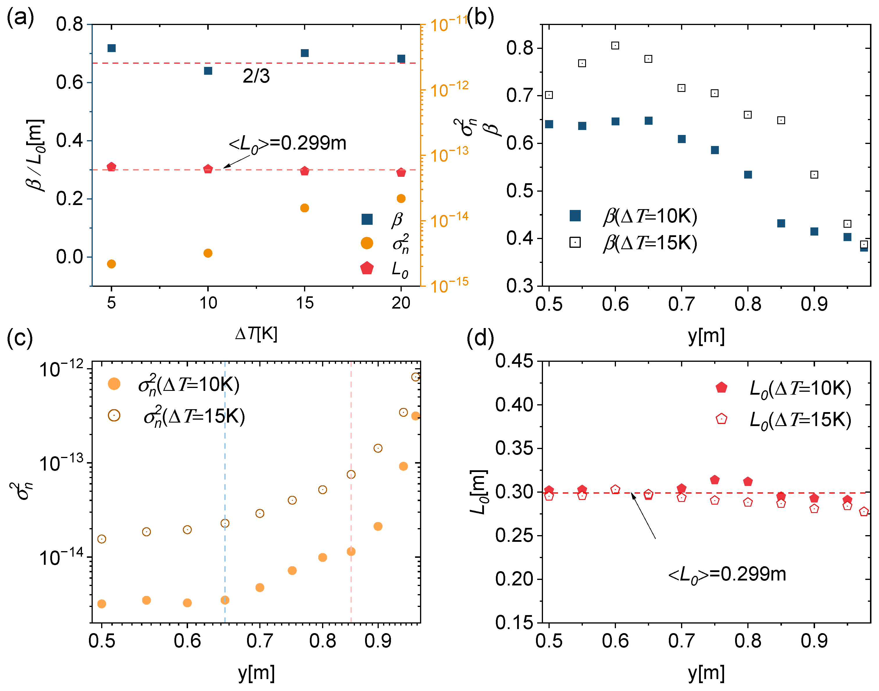
Figure 13 shows the refractive index variance obtained by direct calculation, the scaling power β , and outer scale L 0 obtained by fitting, where Figure 13a shows the variation of refractive index variance σ n 2 , scaling power β and outer scale L 0 , with temperature difference for a horizontal cross-section of y = 0.5 m. The refractive index variance σ n 2 increases with temperature difference, and the change in scaling power β changes slightly with altitude with increasing temperature difference (5–20 K), the outer scale L 0 shows a slight decreasing tendency with increasing temperature difference, and its average value is 0.299 m. Also, as shown in Figure 13d, there is no significant change in the outer scale L 0 at different locations, only with a slight decrease in the outer scale L 0 in the near-boundary region. The variation of the scaling power β at different locations is shown in Figure 13b, where the scaling power β shows large fluctuations as the distance away from the center increases, with a quick decrease in the scaling power β starting from y = 0.7 m, and the closer the region is to the boundary, the smaller the scaling power β becomes. This indicates that the RB turbulence simulator is closer to Kolmogorov turbulence only in the region close to the center bulk, and the turbulence gradually deviates from Kolmogorov turbulence as the distance away from the center increases, and its turbulence is non-Kolmogorov turbulence in the near-boundary large-scale circulation region.
It is worth noting the trend of the refractive index variance σ n 2 with the increase of the distance from the center position. The refractive index variance σ n 2 profiles at both 10 K and 15 K show three marked variations in the log-log graph, the refractive index variance σ n 2 fluctuation near the center region is small, and with the increase of the distance shows a logarithmic distribution, and in the region near the boundary shows a power law distribution. This shows that the upper and lower plates have a remarkable effect on the turbulence intensity, and the refractive index variance σ n 2 profile varies more significantly with height, it is necessary to make a reasonable choice of the aperture of the turbulence simulator when designing so that the edge of the laser beam will not produce large fluctuations.

8. Conclusions

Many studies on the optical properties of turbulence simulators focus more on the turbulence intensity in the light propagation path in the center of the turbulence simulator, and no study has yet comprehensively analyzed the change of optical turbulence intensity with different spatial locations. A detailed investigation of the optical structure inside the turbulence simulator is of great significance for the development of better optical turbulence basic research and applications. In this article, the LES method is employed to thoroughly analyze the spatial structural properties of optical turbulence within the RB turbulence simulator. The refractive index field can be calculated from the three-dimensional temperature, pressure, and density fields obtained by LES. The structural characteristics of two-dimensional longitudinal sections of C n 2 distribution, r 0 at different heights, the refractive index PSD, the profiles of the refractive index variance, the scaling power, and the turbulence outer scale have been investigated in detail. The results show that the hot and cold plumes and the large-scale circulation strongly influence the inhomogeneity of C n 2 in the turbulence tank. The convection cells’ roll-like structure suggests a core region along the center of the tank, and the turbulence strength in the core area is significantly smaller than that in the boundary region. Meanwhile, with the increase in temperature difference, turbulence strength on the longitudinal section keeps rising. The Fried parameter r 0 and the variance of C n 2 distribution along the y-axis also confirm the existence of a calm central region, which is attributed to convective plumes near the upper and lower boundaries. As the temperature difference gradually increases, the turbulent field energy keeps increasing and the velocity of the convective cell gradually increases, which leads to a gradual decrease of the r 0 value. The refractive index power spectrum along the propagation direction exhibits up–down symmetry for the center, and the power spectral density gradually deviates from the −5/3 scaling power because of the increasing distance from the central region. We quantified the degree of this deviation using the profiles of the refractive index variance, the scaling power, and the outer scale with height. It is worth noting that under the log-log plot, the variation of the refractive index variance with height exhibits a three-segmented feature, showing in order a gently increasing region as the distance from the center increases, a logarithmic profile, and a power-law profile in the region close to the boundary. This research will give an important insight into the spatial structure of optical turbulence inside the turbulence simulator, which in turn will provide a well-established platform for testing applications such as free-space optical communication, high-energy laser propagation, remote sensing, and so on.

Author Contributions

Conceptualization, Y.L.; methodology, R.R.; software, Y.L. and S.Y.; validation, S.Y. and Z.T.; formal analysis, Y.L.; investigation, H.D.; resources, H.M.; data curation, Y.L.; writing—original draft preparation, Y.L.; writing—review and editing, Y.L.; visualization, Y.L.; supervision, R.R.; project administration, H.M.; funding acquisition, X.W. All authors have read and agreed to the published version of the manuscript.

Funding

This research was funded by National Natural Science Foundation of China (NSFC), grant number 12302514, 62301530; the HFIPS Director’s Foundation, grant number YZJJ2023QN05; Open Fund of Infrared and Low Temperature Plasma Key Laboratory of Anhui Province, NUDT, grant number IRKL2023KF05; the Major Research plan of the National Natural Science Foundation of China, grant number 91752103.

Data Availability Statement

Data will be made available on request.

Conflicts of Interest

The authors declare no conflicts of interest.

References

  1. Strohbehn, J.W. Laser Beam Propagation in the Atmosphere; Springer: Berlin/Heidelberg, Germany, 1978. [Google Scholar]
  2. Tatarskii, V.I.; Ishimaru, A.; Zavorotny, V.U. Wave Propagation in Random Media (Scintillation); SPIE: Bellingham, WA, USA, 1993. [Google Scholar]
  3. Andrews, L.C.; Phillips, R.L. Laser Beam Propagation through Random Media; SPIE: Bellingham, WA, USA, 1998. [Google Scholar]
  4. Kalensky, M.; Spencer, M.F.; Jumper, E.J.; Gordeyev, S. Estimation of atmospheric optical turbulence strength in realistic airborne environments. Appl. Opt. 2022, 61, 6268–6279. [Google Scholar] [CrossRef] [PubMed]
  5. Bashkansky, M.; Lucke, R.L.; Funk, E.; Rickard, L.J.; Reintjes, J. Two-dimensional synthetic aperture imaging in the optical domain. Opt. Lett. 2002, 27, 1983–1985. [Google Scholar] [CrossRef] [PubMed]
  6. Matt, S.; Hou, W.; Goode, W.; Hellman, S. Introducing SiTTE: A controlled laboratory setting to study the impact of turbulent fluctuations on light propagation in the underwater environment. Opt. Express 2017, 25, 5662–5683. [Google Scholar] [CrossRef] [PubMed]
  7. Majumdar, A.K.; DiUbaldo, J.A.; Brown-VanHoozer, A. Measurement and characterization of laboratory-simulated turbulence parameters of interest to adaptive optics imaging and laser communications. In High-Resolution Wavefront Control: Methods, Devices, and Applications; SPIE: Bellingham, WA, USA, 1999; Volume 3760, pp. 123–128. [Google Scholar]
  8. Majumdar, A.K.; Gamo, H. Statistical Measurements of Irradiance Fluctuations of a Multipass Laser-Beam Propagated through Laboratory-Simulated Atmospheric-Turbulence. Appl. Opt. 1982, 21, 2229–2235. [Google Scholar] [CrossRef]
  9. Rickenstorff, C.; Rodrigo, J.A.; Alieva, T. Programmable simulator for beam propagation in turbulent atmosphere. Opt. Express 2016, 24, 10000–10012. [Google Scholar] [CrossRef] [PubMed]
  10. Yuan, R.M.; Sun, J.N.; Luo, T.; Wu, X.P.; Wang, C.; Lu, C. Simulation study on light propagation in an isotropic turbulence field of the mixed layer. Opt. Express 2014, 22, 7194–7209. [Google Scholar] [CrossRef] [PubMed]
  11. Yuan, R.M.; Sun, J.N.; Luo, T.; Wu, X.P.; Wang, C.; Fu, Y.F. Simulation study on light propagation in an anisotropic turbulence field of entrainment zone. Opt. Express 2014, 22, 13427–13437. [Google Scholar] [CrossRef]
  12. Nootz, G.; Matt, S.; Kanaev, A.; Judd, K.P.; Hou, W.L. Experimental and numerical study of underwater beam propagation in a Rayleigh-Benard turbulence tank. Appl. Opt. 2017, 56, 6065–6072. [Google Scholar] [CrossRef]
  13. Lohse, D.; Xia, K.Q. Small-Scale Properties of Turbulent Rayleigh-Benard Convection. Annu. Rev. Fluid Mech. 2010, 42, 335–364. [Google Scholar] [CrossRef]
  14. Matt, S.; Nootz, G.; Hellman, S.; Hou, W. Effects of Optical Turbulence and Density Gradients on Particle Image Velocimetry. Sci. Rep. 2020, 10, 2130. [Google Scholar] [CrossRef]
  15. Renmin, Y.; Jie, M.; Hao, L.; Xuping, W.; Jianning, S.; Xiaoling, J. Simulation of the microstructural characteristics of saltwater turbulence in a water tank. Opt. Express 2018, 26, A844–A854. [Google Scholar] [CrossRef] [PubMed]
  16. Gulich, D. Temporal correlations imaging fixed targets through turbulence. Opt. Lett. 2016, 41, 2855–2858. [Google Scholar] [CrossRef] [PubMed]
  17. Funes, G.; Olivares, F.; Weinberger, C.G.; Carrasco, Y.D.; Nunez, L.; Perez, D.G. Synthesis of anisotropic optical turbulence at the laboratory. Opt. Lett. 2016, 41, 5696–5699. [Google Scholar] [CrossRef] [PubMed]
  18. Ferlic, N.A.; Avramov-Zamurovic, S.; O’Malley, O.; Judd, K.P.; Mullen, L.J. Synchronous optical intensity and phase measurements to characterize Rayleigh-Benard convection. J. Opt. Soc. Am. A Opt. Image Sci. Vis. 2023, 40, 1662–1672. [Google Scholar] [CrossRef] [PubMed]
  19. Benitez, E.K.; Borg, M.P.; Hill, J.L.; Aultman, M.T.; Duan, L.; Running, C.L.; Jewell, J.S. Quantitative focused laser differential interferometry with hypersonic turbulent boundary layers. Appl. Opt. 2022, 61, 9203–9216. [Google Scholar] [CrossRef] [PubMed]
  20. Rasouli, S.; Mohammadi Razi, E.; Niemela, J.J. Investigation of the anisotropy and scaling of the phase structure function of a spatially coherent light beam propagating through convective air turbulence. J. Opt. Soc. Am. A 2022, 39, 1641–1649. [Google Scholar] [CrossRef]
  21. Kaczorowski, M.; Chong, K.L.; Xia, K.Q. Turbulent flow in the bulk of Rayleigh-Benard convection: Aspect-ratio dependence of the small-scale properties. J. Fluid Mech. 2014, 747, 73–102. [Google Scholar] [CrossRef]
  22. Pandey, A.; Scheel, J.D.; Schumacher, J. Turbulent superstructures in Rayleigh-Benard convection. Nat. Commun. 2018, 9, 2118. [Google Scholar] [CrossRef]
  23. Bhattacharya, S.; Verma, M.K.; Samtaney, R. Prandtl number dependence of the small-scale properties in turbulent Rayleigh-Benard convection. Phys. Rev. Fluids 2021, 6, 063501. [Google Scholar] [CrossRef]
  24. Wang, Q.; Verzicco, R.; Lohse, D.; Shishkina, O. Multiple States in Turbulent Large-Aspect-Ratio Thermal Convection: What Determines the Number of Convection Rolls? Phys. Rev. Lett. 2020, 125, 074501. [Google Scholar] [CrossRef]
  25. Schneide, C.; Pandey, A.; Padberg-Gehle, K.; Schumacher, J. Probing turbulent superstructures in Rayleigh-Benard convection by Lagrangian trajectory clusters. Phys. Rev. Fluids 2018, 3, 113501. [Google Scholar] [CrossRef]
  26. Aghighi, M.S.; Ammar, A.; Metivier, C.; Gharagozlu, M. Rayleigh-Benard convection of Casson fluids. Int. J. Therm. Sci. 2018, 127, 79–90. [Google Scholar] [CrossRef]
  27. Wang, Q.; Xia, S.N.; Yan, R.; Sun, D.J.; Wan, Z.H. Non-Oberbeck-Boussinesq effects due to large temperature differences in a differentially heated square cavity filled with air. Int. J. Heat Mass. Transf. 2019, 128, 479–491. [Google Scholar] [CrossRef]
  28. Paolucci, S.; Chenoweth, D.R. Transition to Chaos in a Differentially Heated Vertical Cavity. J. Fluid Mech. 1989, 201, 379–410. [Google Scholar] [CrossRef]
  29. Kimmel, S.J.; Domaradzki, J.A. Large eddy simulations of Rayleigh-Benard convection using subgrid scale estimation model. Phys. Fluids 2000, 12, 169–184. [Google Scholar] [CrossRef]
  30. Pierre, S. Large Eddy Simulation for Incompressible Flows. An Introduction. Meas. Sci. Technol. 2001, 12, 1745. [Google Scholar]
  31. Smagorinsky, J. General Circulation Experiments with the Primitive Equations: I. The Basic Experiment. Mon. Weather Rev. 1963, 91, 99–164. [Google Scholar] [CrossRef]
  32. Huang, X.J.; Zhang, L.; Hu, Y.P.; Li, Y.R. Large eddy simulation on Rayleigh-Benard convection of cold water in the neighborhood of the maximum density. Fluid Dyn. Res. 2018, 50, 035503. [Google Scholar] [CrossRef]
  33. Scheel, J.D.; Kim, E.; White, K.R. Thermal and viscous boundary layers in turbulent Rayleigh-Benard convection. J. Fluid Mech. 2012, 711, 281–305. [Google Scholar] [CrossRef]
  34. Schmidt, J.D. Numerical Simulation of Optical Wave Propagation with Examples in MATLAB; SPIE: Bellingha, WA, USA, 2010. [Google Scholar]
  35. Rao, R.Z. Description and measurement of the strength of an optical turbulence. In Optics in Atmospheric Propagation and Adaptive Systems VII; SPIE: Bellingha, WA, USA, 2004; Volume 5572, pp. 45–48. [Google Scholar]
Figure 1. (a) Schematic of the geometric model of the turbulence simulator, (b) Variation of the Nusselt number with time obtained by the LES, (c) Variation of the Nusselt number with Rayleigh number obtained by the LES.
Photonics 11 00229 g001
Figure 2. The instantaneous temperature field on the longitudinal section parallel to the long axis of the turbulence tank at (a) 20 s, (b) 100 s, (c) 300 s, and (d) 400 s under a temperature difference of 15 K.
Photonics 11 00229 g002
Figure 3. The instantaneous temperature field at Δ T = 15   K , t = 455 s, for different x: (a) x = 0.05 m, (b) x = 0.45 m, (c) x = 0.55 m, (d) x = 0.95 m.
Photonics 11 00229 g003
Figure 4. The instantaneous temperature field in the transverse plane perpendicular to the long axis at Δ T = 15   K , t = 455 s, for different z: (a) z = 0.05 m, (b) z = 0.45 m, (c) z = 0.55 m, (d) z = 0.95 m.
Photonics 11 00229 g004
Figure 5. Transient temperature field in the x-z plane at different locations for a temperature difference of 15 K, t = 455 s: (a) y = 0.05 m, (b) y = 0.45 m, (c) y = 0.55 m, (d) y = 0.95 m.
Photonics 11 00229 g005
Figure 6. Horizontal cross-sections at different heights in the turbulence simulator for different temperature differences. (a1) Δ T = 5   K ,   y = 0.50   m , (b1) Δ T = 5   K ,   y = 0.75   m , (c1) Δ T = 5   K ,   y = 0.95   m , (a2) Δ T = 10   K ,   y = 0.50   m , (b2) Δ T = 10   K ,   y = 0.75   m , (c2) Δ T = 10   K ,   y = 0.95   m , (a3) Δ T = 15   K ,   y = 0.50   m , (b3) Δ T = 15   K ,   y = 0.75   m , (c3) Δ T = 15   K ,   y = 0.95   m , (a4) Δ T = 20   K ,   y = 0.50   m , (b4) Δ T = 20   K ,   y = 0.75   m , (c4) Δ T = 20   K ,   y = 0.95   m .
Photonics 11 00229 g006
Figure 7. Distributions at different locations in the yz-plane, which denote the C n 2 distributions: (a) near the lower boundary region, (b) the center region, and (c) the region near the upper boundary.
Photonics 11 00229 g007
Figure 8. Distribution at different locations in the xz-plane, which represents the C n 2 distribution: (a) near the lower boundary region, (b) the center region, and (c) the upper boundary region.
Photonics 11 00229 g008
Figure 9. In the horizontal cross-sections under different temperature conditions: (a) 5 K, (b) 10 K, (c) 15 K, (d) 20 K.
Photonics 11 00229 g009
Figure 10. Variation of r 0 with height in a turbulence simulator for different temperature differences Δ T .
Photonics 11 00229 g010
Figure 11. Variation of spatial refractive index power spectral density with height for different temperature conditions, where the scatter plot represents the simulated data and the line represents the fitted curve for the −5/3 scale rate. (a) 5 K, (b) 10 K, (c) 15 K, (d) 20 K.
Photonics 11 00229 g011
Figure 12. (a) Influence of the temperature difference between the top and bottom plates of the turbulence simulator on the refractive structure function in the center region of the flow field in the horizontal direction; (b) influence of the spacing from the bottom plate on the refractive index structure function in the horizontal direction, where the solid line indicates the LES data and the dashed line indicates the fitted data.
Photonics 11 00229 g012
Figure 13. (a) Variation of scaling power β , and outer scale L 0 and refractive index variance σ n 2 with temperature difference in the x-z plane at y = 0.5 m; (b) variation of scaling power β with spatial height; (c) profile of refractive index variance with increasing altitude; (d) profiles of outer scale L 0 with increasing altitude.
Photonics 11 00229 g013
Table 1. Simulation parameters.
PrTh [K]Tc [K] N x × N y × N z ΔT [K]Ra
0.7293.15298.15200 × 200 × 24054.7 × 108
0.7293.15303.15200 × 200 × 240109.4 × 108
0.7293.15308.15200 × 200 × 240151.4 × 109
0.7293.15313.15200 × 200 × 240201.8 × 109
Disclaimer/Publisher’s Note: The statements, opinions and data contained in all publications are solely those of the individual author(s) and contributor(s) and not of MDPI and/or the editor(s). MDPI and/or the editor(s) disclaim responsibility for any injury to people or property resulting from any ideas, methods, instructions or products referred to in the content.