Article

Nanoscale Dots, Grids, Ripples, and Hierarchical Structures on PET by UV Laser Processing

1
Institute of Biomedical Mechatronics, Johannes Kepler University Linz, 4040 Linz, Austria
2
Institute of Applied Physics, Johannes Kepler University Linz, 4040 Linz, Austria
3
Center for Surface and Nanoanalytics, Johannes Kepler University Linz, 4040 Linz, Austria
*
Author to whom correspondence should be addressed.
Photonics 2024, 11(2), 184; https://doi.org/10.3390/photonics11020184
Submission received: 22 December 2023 / Revised: 1 February 2024 / Accepted: 9 February 2024 / Published: 18 February 2024
(This article belongs to the Special Issue Emerging Trends in Laser Processing Techniques)

Abstract

:
Nanostructures can be produced on poly(ethylene terephthalate) (PET) foils by using a krypton fluoride (KrF) excimer laser with a wavelength of 248 nm and a pulse duration of about 20 ns. We show that surface nanoripples, nanodots, nanogrids, and hybrid patterns of ripples with dots or finer ripples on top can be fabricated. The effects of a water layer in front of the PET foil and of cooling during laser processing were investigated. For pattern formation, several irradiation parameters (pulse number, pulse energy, and polarization) were varied systematically. The spatial periods of the ripples were changed by adjusting the angle of incidence of the laser beam. All nanostructures were characterized by scanning electron microscopy, and relevant morphological parameters, such as peak-to-peak distances and spatial periods, were assessed. Shapes and heights of some structures were characterized by using focused ion beam cuts to avoid the tip-sample convolution effects typical of atomic force microscopy images. We further demonstrate nanoripple formation on PET foils as thin as 12 µm, 6 µm, and 1.4 µm. The remarkable variety of nanostructures on PET we present here enables customized fabrication for a wide range of applications.

1. Introduction

Nature makes abundant use of highly versatile nano- and microscale surface features [1,2,3] for antiadhesion [4,5], wetting [6,7], directional liquid transport [8,9], and structural color [10,11]. All these surface properties are strongly influenced by the specific designs of the corresponding structures. Thus, in biomimicry, controlling the surface morphology is key to optimizing for a specific application [12]. Laser processing enables micro- and nanostructuring of areas of several square centimeters on widely used technical polymeric materials without the need for a clean room or mask fabrication [13,14]. In addition to their use in nanostructuring of polymer films [14], the unique capabilities of ultraviolet (UV) lasers, such as krypton fluoride (KrF) excimer lasers, make for a wide range of application areas, including the growth of thin films by pulsed laser deposition (PLD) [15], the synthesis of nanocrystals [16], and the creation of photosensitive two-dimensional structures by reactive PLD [17].
Under certain conditions, irradiation with polarized laser light generates self-organized nanoripples on surfaces [14,18,19,20]. These nanoripples are widely known as laser-induced periodic surface structures (LIPSS) and are a universal phenomenon [21]. Their fabrication on polymers such as poly(ethylene terephthalate) (PET) [14,22,23,24,25,26,27,28,29] requires thousands of nanosecond (ns) UV laser pulses of linearly polarized light on the same spot. The fluence of the pulses needs to be well below the single-pulse ablation threshold of the material. A simple theory [19,30] explains the emergence of nanoripples as associated with the incident laser beam interfering with the light scattered by the rough polymer surface. In the case of PET, the nanoripples are in parallel alignment with the direction of linear polarization.
Using s-polarization (also called σ-polarization), the spatial period Λ of LIPSS is given by
Λ = λ / n e f f sin θ ,
and, thus, depends on the angle of incidence θ of the laser light, the wavelength of the laser light, and the effective refractive index n e f f [19,26,31]. The lower and upper limits of n e f f are, respectively, the refractive indices of air and of the base material. From a mathematical point of view, perfectly regular nanoripples can be described as periodic functions because their shapes repeat. The spatial period Λ is the distance between consecutive positions at which the nanoripples have the same shape, for example, between consecutive peaks. The effective refractive index for PET was calculated to be 1.235 ± 0.053 (±4.3%) at an average fluence of approximately 5.7 to 6.2 mJ/cm2 when using a ns KrF excimer laser [32]. The emergence of LIPSS needs a positive feedback mechanism, such as a temperature field [19].
In [32], increasing the angle of incidence from 0° to 60° generated LIPSS with spatial periods in the range of ~214 nm to ~613 nm on 50 μm thick PET foils. The values measured were in accordance with Equation (1). A similar experiment with 50 μm thick PET foils was performed using a xenon chloride (XeCl) excimer laser with a wavelength λ of 308 nm [31]. The spatial periods ranged from 250 nm to 850 nm, which means that the total range was wider due to the lower effective refractive index and the starting spatial period was larger due to the higher wavelength. The experimental data were also in agreement with Equation (1). In this experiment, neff = 1.17 ± 0.01 served as a fit parameter.
LIPSS on polymers such as PET and their morphology have been thoroughly studied in recent decades [14,22,23,28,29]. Rodríguez-Beltrán et al. reported the formation of LIPSS on PET and PET/Expanded Graphite (EG) films [23]. They employed laser irradiation with ns laser pulses at 266 nm using the fourth harmonic beam from a Q-Switched Nd:YAG system. Among other physicochemical properties, the spatial periods and heights of the resulting nanoripples were studied as functions of the pulse numbers used. Cui et al. [22] studied the effects of film and substrate thickness on LIPSS formation on poly(styrene) (PS) films, using the aforementioned laser system. They found that thinner (<200 nm) and thicker (>400 nm) films developed well-ordered LIPSS, while those with intermediate thicknesses (200–400 nm) formed distorted LIPSS with drop-like structures. Nanoripples on PET with various spatial periods were studied, employing, again, the 266 nm—ns laser and alternatively a 193 nm—ns argon fluoride (ArF) excimer laser [29] or a 248 nm—ns KrF excimer laser [32]. While elliptically polarized light also resulted in ripples, the use of circularly polarized light gave rise to rounded structures with sizes close to the laser wavelength, thus extending structural variability. PET fibers were modified by both high [33] and low [34] fluences, resulting in micrometer-sized and submicrometer-sized ripples, respectively. Underwater laser treatment with a KrF excimer laser yielded “worm”-like structures on PET [35], and on photoresist, it resulted in similar corrugated ripples independent of the direction of the laser polarization [36,37]. In general, morphological changes of PET upon laser treatment were accompanied by chemical surface modification [29,35,38,39].
Bioinspired LIPSS on PET were shown to significantly reduce the adhesion of Escherichia coli bacteria [32] (~−91%) and nanofibers [4] (about −73% when combined with a gold coating) compared to the unstructured pristine surfaces. Other applications of LIPSS on PET include the formation of gold nanowires [24,27,40] for localized plasmon voltammetry sensing [40], the preparation of silver nanowires [41], and the activation of human microvascular endothelial cells (HMECs) [24].
For each current and future application field, structural morphology needs to be optimized, which in turn requires its characterization to be as good as possible. Topographical characterization of bioinspired LIPSS by atomic force microscopy (AFM) was shown to be affected by tip-sample convolution effects in [5], where these effects were most probably due to the high aspect ratios of the structures fabricated, and the steep slopes of their edges that made topography assessment by AFM more challenging. For certain example LIPSS structures processed under the same conditions, focused ion beam (FIB) cuts [4] gave larger structural heights than AFM images [32]. Furthermore, the ripples seemed considerably wider in AFM images [32] than in scanning electron microscopy (SEM) recordings and FIB cuts [4].
In this work, we aimed to broaden the variability and improve our understanding of nanoscale structures on 50 μm thick PET foils obtained by ns UV laser processing using a KrF excimer laser at a wavelength of 248 nm. To this end, we studied the influences of the angle of incidence, fluence, number of pulses, two directions of polarization, foil thickness, a water layer in front of the substrate, and substrate cooling on the structures obtained. Further, we succeeded in fabricating nanoripples on PET foils as thin as 12 µm, 6 µm, and 1.4 µm with the help of substrate support foils [42,43]. We thus manipulated the spatial periods of the ripples, their shapes and heights, even—to some extent—independently of each other. To have full access to ripple topography without any influences of the tip-sample convolution effects typical of AFM we used FIB cuts for characterization. Nanodots instead of nanoripples emerged below a particular fluence value. Above a specific fluence range, the structures became more complex than simple nanoripples. First, a finer ripple structure formed on top of the main nanoripples, which then differentiated further into diamond-like structures. The superposition of two independent directions of polarization resulted in self-assembled nanogrids and nanoripples with nanodots on top, which resembled pearl chains. A water layer changed the overall morphology of the structures: their regularity and their spatial periods. Substrate cooling below 0 °C, however, suppressed the creation of nanoripples or decreased their heights depending on the fluence applied.
This work presents, to the best of our knowledge, for the first time: (i) systematic analysis of LIPSS heights and shapes on PET using FIB cuts and thus completely eliminating the tip-sample convolution effects typical of AFM; (ii) LIPSS formation on very thin foils with thicknesses of some microns (hitherto only ultrathin films had been used); (iii) nanogrids and hierarchical structures on PET, such as nanoripples with nanodots on top, were fabricated by successively superimposing two directions of linear polarization; (iv) low-fluence nanodot formation on PET by using the linearly polarized light of a KrF excimer laser; (v) LIPSS formation on PET with a water layer in front of the foil during laser processing; and (vi) suppression of LIPSS formation on PET by cooling of the substrate. We were able to modify and broaden the spectrum of nanostructures achievable on PET. Furthermore, we refined the assessment of ripple characteristics by using FIB cuts. Possible applications of our findings are the fabrication of advanced surfaces that are anti-adhesive to nanofibers [4,5] or repel bacteria [32]. Furthermore, they might be used for improvements to localized plasmon voltammetry sensing [40], in biomimicry [1,3,12], and in the biomedical context [44,45,46], for instance, to activate cells [24,29]. We expect the main ideas presented in this paper to be transferable to poly(styrene) (PS) [24,47] and SU-8 thin films [48,49] because these materials have shown similar nanoripples at comparable fluences and wavelengths.

2. Materials and Methods

2.1. Fabrication of Structures on PET

2.1.1. Materials

Unless stated otherwise, 50 μm thick, flat, biaxially stretched PET foils (Goodfellow Ltd., Bad Nauheim, Germany) served as substrate. To simplify handling of these fragile, ultrathin PET foils (1.4 μm thin Mylar CW02, 6 μm thin Mylar C, and 12 μm thin Mylar C; Pütz GmbH + Co. Folien KG, Taunusstein, Germany), they were attached to a reusable support substrate foil—a silicone display protection foil similar to the support foils described in [42,43].

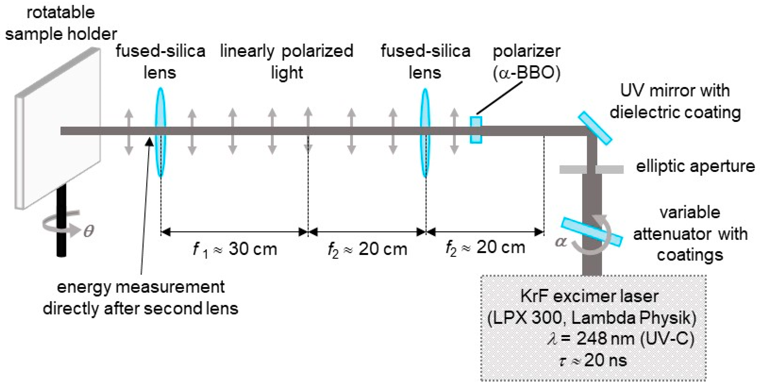
2.1.2. General Setup for Varying the Angle of Incidence, Pulse Number, and Fluence

Nanoscale structures were fabricated using a ns KrF excimer laser (LPX 300, Lambda Physik, Göttingen, Germany) (Figure 1) with a wavelength of λ = 248 nm and a pulse duration τ of approx. 20 ns. This setup was also employed in [4,5,32] for LIPSS formation. For all samples presented in this work, the pulse repetition rate was set to ν = 10 Hz in the laser control software. For all samples (except for those with irregular ripples), an operating voltage of 22 kV was chosen in the software. The laser light was linearly polarized by α-BBO polarizers from either Melles Griot, Carlsbad, CA, USA (for irregular ripples and variation of the angles of incidence, some of the thinner PET foils, the cooled samples, and those fabricated at elevated fluences) or Thorlabs GmbH, Bergkirchen, Germany (for all other parameter combinations studied).
A high-power variable attenuator with a dielectric coating (magnetron sputtered and with an antireflection coating, Laseroptik GmbH, Garbsen, Germany) mounted on an electronically controlled, rotatable stepper motor was used to adjust the pulse energies E. An elliptic aperture was placed after the attenuator. A telescope formed by two fused-silica lenses imaged the output of the polarizer onto the PET foils that had been fixed to a rotatable sample holder with adhesive tape. During the experiments, the homogeneity of the laser beam directly after the attenuator and directly after the elliptic aperture was regularly monitored. This way, the position of the elliptic aperture was optimized to reach maximal homogeneity of the laser beam.
The rotatable sample holder allowed the influence of the angle of incidence θ on ripple formation to be studied. The fluence ϕ = Eθ/Aθ, with Eθ the pulse energy and Aθ the area of the laser spot, was kept constant. To this end, the pulse energy Eθ and the angle of incidence θ needed to increase simultaneously, since the area of the laser spot Aθ grows according to the formula Aθ = A/cosθ with the increasing angle of incidence θ. At an angle of incidence θ = 0°, the laser hit the sample at a right angle and the area processed was the smallest, denoted by A. The size of a reference processed area (A30° processed with θ = 30°) was used to calculate the pulse energy necessary to achieve a particular fluence at a certain angle. The area was measured using the free open-source computer program Fiji [50] (version 1.53q; it is an ImageJ2 distribution developed by Wayne Rasband and coworkers, National Institutes of Health, Bethesda, MD, USA). To measure the area value given in Section 3.1.1., laser-processed areas of five different samples were copied onto pieces of transparent pristine PET foils using a permanent marker pen. Subsequently, they were placed on graph paper and photographs were taken with a standard mobile phone. The photographs were scaled with the “Set scale” function in Fiji and then the margins were traced with the “Polygon selections” function. The areas within the margins were calculated using “Measure” from the “Analyze” tab in Fiji. Depending on the angle of incidence θ and the polarizer used, the size of the laser-processed area was between one and three square centimeters. Fluence values were chosen by adjusting the corresponding pulse energies to the size of the processed area, considering the formulas above, and by using the attenuator and the energy measurement device previously described.

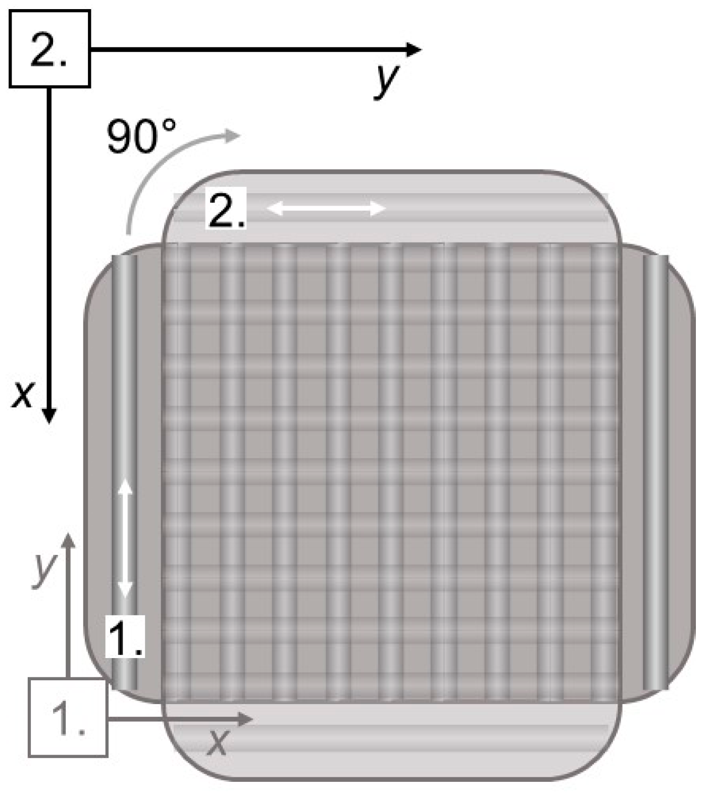
2.1.3. Adaptations and Amendments of the Setup for Fabrication of Irregular Ripples, Water Layer Usage, Substrate Cooling, and Superposition of Two Polarization Directions

For the formation of irregular nanoripples, no lenses, no polarizer, and N = 6000 pulses were used. To this end, a second beamline was established, where a fixed sample holder was aligned perpendicular to the laser beam, i.e., the angle of incidence was set to θ = 0°. Since there was no telescope configuration present in this beamline, the processed area was smaller in size. Despite that, the fluence Φ could be kept at approximately 5.7 to 6.2 mJ/cm2 by operating the laser at 18 kV (instead of 22 kV) and by using the aforementioned variable attenuator. For adaption purposes, the pulse energy was measured directly before the fixed sample holder using the aforementioned joulemeter.
A customized rotatable sample holder bore a layer of distilled water in front of the PET samples; a photograph of the sample holder is shown in Section 3.1.5. Spacers enabled to regulate the thickness of the layer; spacers for 2 mm, 4 mm, 6 mm, and 7.9 mm thick layers were available.
For substrate cooling, a Peltier element (model: RC12-6L, II-VI Marlow, division of Coherent Corporation, Saxonburg, PA, USA) was clued to an aluminum heat sink with a thermally conducting adhesive. A fan for cooling the hot side was mounted onto the heat sink. The equilibrium state with a constant temperature was awaited. The temperature of the PET foil was measured with an infrared temperature sensor (model: PC151LT-0, Calex, Leighton Buzzard, England, Great Britain; accuracy of ±1 °C or ±1% of reading) after the water which had condensed from ambient air had been wiped off with a lens cleaning tissue (Assistent, article number: 41019010, Glaswarenfabrik Karl Hecht GmbH & Co KG, Sondheim vor der Rhön, Germany). However, it could not be completely excluded that a thin water layer was present during the measurements. Directly before laser treatment, the thin water layer was wiped off again with the lens-cleaning tissue.
To superimpose two directions of linear polarization (Figure 2), first, the PET was processed with the linear polarization in parallel to the y-direction. Then, the foil was rotated by 90° and mounted on the sample holder again. After that, it was exposed to the laser light with the linear polarization parallel to the x-direction.

2.2. Scanning Electron Microscopy (SEM) Images

Before SEM imaging (model REM 1540XB Crossbeam, Zeiss, Oberkochen, Germany), a gold layer with a thickness of 8 to 10 nm was deposited using a sputter coater (AE1230, EMScope, Ashford, England, Great Britain; 3 min at a deposition current of 20 mA and a power of 14.3 W). Conductive silver paste (Leitsilber 200, Österreichische Gold-und Silber-Scheideanstalt Ges.m.b.H., Wien, Austria) was applied to establish electrical contact with the sample holder and to mount the samples on it. For SEM imaging, no stage tilt was used, working distances were between 5 mm and 8 mm, and acceleration (or electron high-tension) voltages of 3 kV were applied. At each position, SEM images with magnifications of 15.17 kx, 41.17 kx, and 143.37 kx were recorded.

2.3. Focused Ion Beam (FIB) Cuts

FIB cuts were used for morphological analysis because in previous studies the shape of the AFM tip caused the surface morphology to be distorted [5], and the resulting measurements of ripple heights were not completely accurate [32]. To prevent charging and improve the contrast between the sample surface and a protective coating, a 12 nm gold layer was applied using a sputter coater (AE1230, EMScope, Ashford, UK; 4 min at a deposition current of 20 mA and a power of 14.3 W). A dot of a black permanent marker pen (Lumocolor, Staedtler Mars GmbH & Co. KG, Nürnberg, Germany) served as a protective deposit at the location of the FIB cut. At the edge of this dot, where the protective layer was less thick than in the center, rectangles or trapezoids of approximately 10–15 µm size were cut into the material with a 1540XB Crossbeam (Zeiss, Oberkochen, Germany) using a milling current of 200 pA–500 pA and an acceleration voltage of 30 kV; this machine merges a GEMINI® field-emission scanning electron microscope utilized for imaging (FE-SEM) with a FIB device used for cutting. The ion source was a Ga+ filament.
The Fiji distribution [50] of the free open-source software ImageJ2 (versions 1.52s and 1.46r) served for evaluation of the FIB cuts. First, the tops and valleys of the nanoripples were identified using the “Multi-point” tool, and then their positions were extracted via the “Measure” tool. The heights of the ripples were calculated using Excel (Microsoft Office 16, Microsoft Cooperation, Redmond, WA, USA) by finding the differences between the tops and valleys. For each height value, the distances between each top and the valleys to its left and right were averaged. The scale bars of the SEM images of the FIB cuts were used to convert all values from pixels to nanometers. Twenty ripples at each position provided the basis to determine the mean values and standard deviations. For the determination of the nanodots’ heights, the same procedure as for the evaluation of the nanoripples’ heights was applied.

2.4. Computation of Morphological Features

2.4.1. Spatial Periods of Regular Ripples

The free software Gwyddion (version 2.55, Czech Metrology Institute, Brno, Czech Republic) was applied to calculate the spatial periods Λ of regular LIPSS on PET, as described in [4,32]. First, SEM micrographs of the samples (magnification of 15.14 k-times) were analyzed using two-dimensional fast Fourier transforms (2D FFT) under default conditions (output type “modulus”, window type “Hann” and “Subtract mean value beforehand”). Depending on their spatial periods and the working distance during SEM imaging, between 15 and 100 ripples were evaluated. Subsequently, profiles were acquired by measuring along the lines that traverse through the resulting peaks. Lorentzian functions with the expression L(k) = y0 + a/[b2 + (kk0)2] served as fit functions for the peaks. In this formula, the position of the peak is represented by k0. The spatial periods Λ were computed from the formula Λ = 2/Δk by using the distances Δk = k0,rightk0,left between the peaks located to the left and right sides of the central peak situated, respectively, at the k0,left and k0,right positions. In case only one position was evaluated and therefore no mean of the results at several positions was computed, the Gaussian law of propagation of uncertainty was applied to determine the errors of the spatial periods from the errors of the peak positions given by Gwyddion’s Lorentzian fit function.

2.4.2. Peak–Peak Distances of Surface Features

In the cases of irregular ripples resulting from leaving out the polarizer or from using a water layer or in the case of finer ripple structures, no distinct peaks were visible in the Fourier transforms. That is why the peak-to-peak distances dpp between the ripples were assessed directly from SEM images. Profiles were extracted along lines perpendicular to the ripples using the free software Gwyddion. Then, the peak-to-peak distances were measured in the resulting graphs with this software.

2.4.3. Areas, Distances, and Radii of Nanodots

The mean radii of the nanodots were computed from the areas assessed by using Gwyddion. First, the “Edit mask” tool was used to color the nanodots red; hereby, the “Freehand mask drawing” tool with a radius of two pixels was applied and voids were filled with the “Fill Voids” action. Then, the “Data process” function “Distributions of various grain characteristics” was employed to compute the projected areas and the equivalent disc radii. The mean distances between the dots were assessed by measuring the center distance(s) between a dot and its nearest neighbor(s), respectively, on the same nanoripple or the nanoripple to the left.

3. Results

3.1. Nanoripples

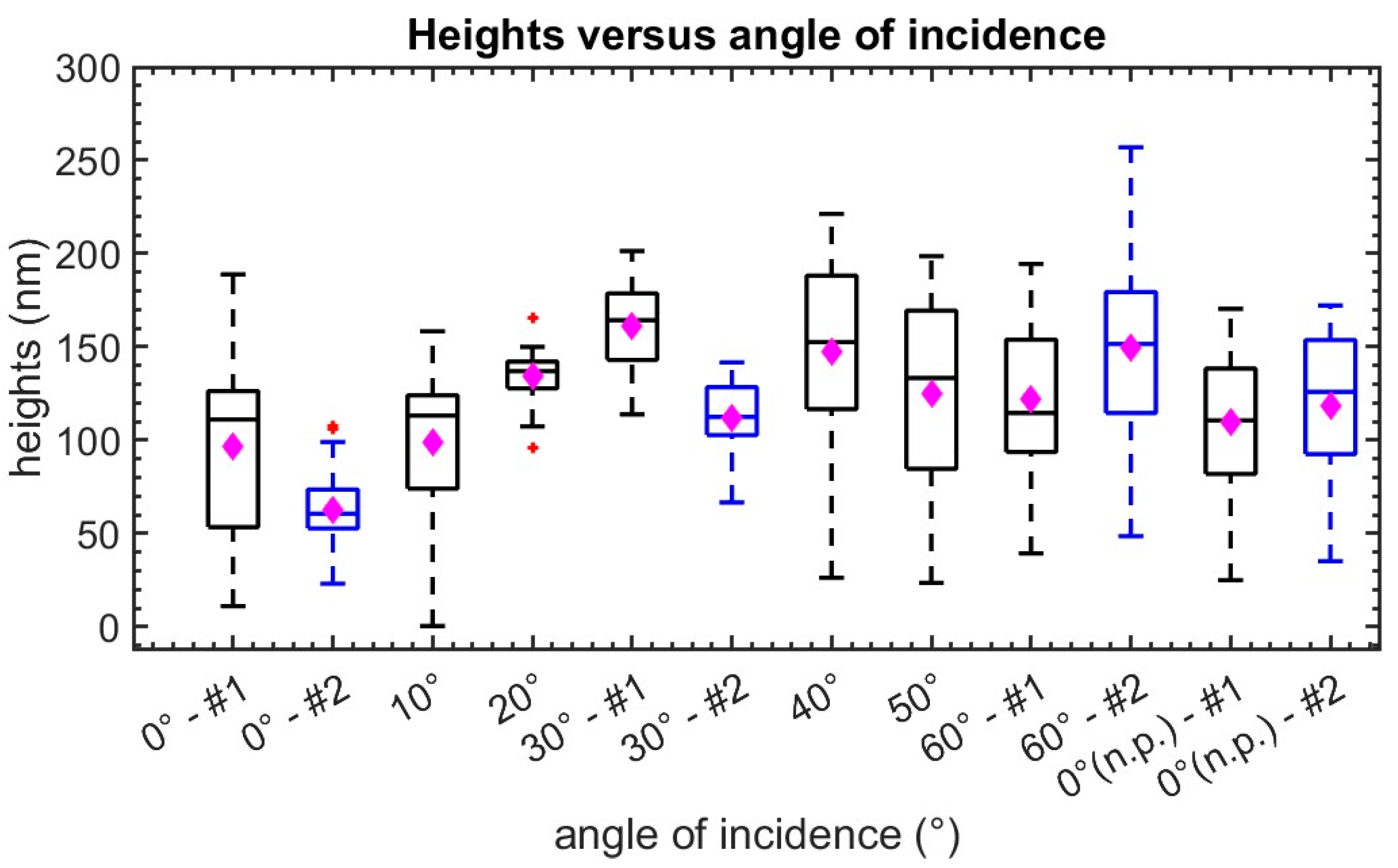
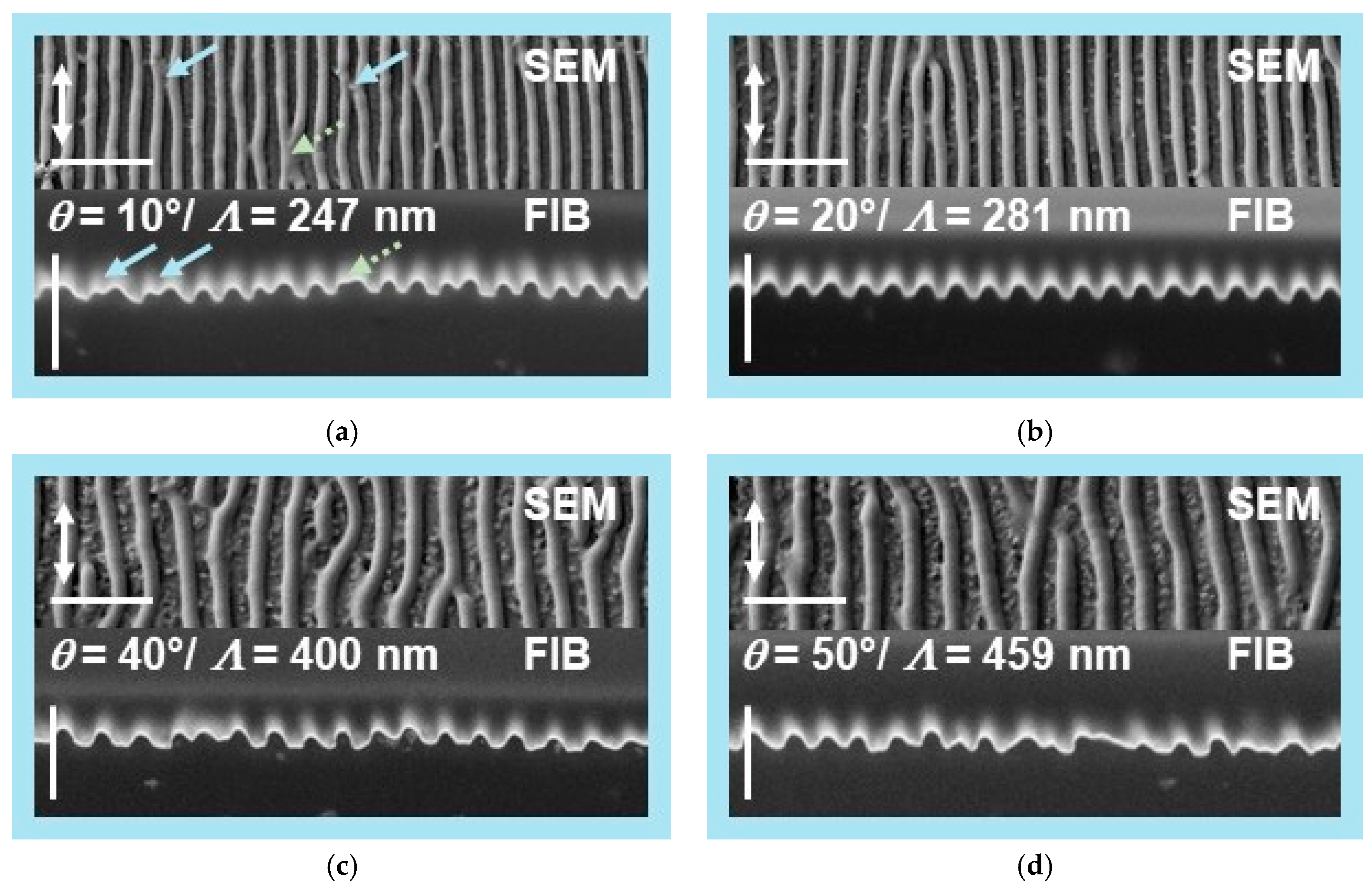
3.1.1. Change in the Angle of Incidence

We assessed the influence of a changing angle of incidence on the ripples’ heights and shapes using FIB cuts. During this study, we maintained a pulse number of N = 6000, an average fluence ϕ of about 5.7 to 6.2 mJ/cm2, and a pulse repetition rate of ν = 10 Hz. For height measurements, twenty ripples were evaluated at each position and angle of incidence. Theoretically, the spatial periods of LIPSS increase with increasing angle of incidence θ following Equation (1). Angles of incidence ranging from 0° to 60° in steps of 10° resulted in ripples with spatial periods of 214 nm, 247 nm, 281 nm, 331 nm, 400 nm, 459 nm, and 613 nm [4,32]. Here, the standard deviations calculated by the Gaussian law of propagation of uncertainty were below 1 nm in all cases. Irregular ripples were generated without a polarizer [4]. Their mean peak-to-peak distance ± standard deviation was 274 nm ± 91 nm (±33%; n = 30), their median value was 250 nm, and their spacings ranged between 130 nm and 480 nm [4].
The heights and shapes of the ripples changed with the spatial periods (Figure 3 and Figure 4). SEM images and FIB cuts revealed that at some angles and positions the ripples were very homogeneous (Figure 3b), while at others, merging and bifurcation often resulted in exceptionally short (light blue arrow) and high (dashed light green arrow) ripples (Figure 3a). Figure 4 displays boxplots of the heights evaluated from FIB cuts at one or two positions on the sample surfaces. The mean heights of the regular ripples slightly increased with the angles of incidence increasing from 0° to 30° and thus with the spatial periods. However, this increase was not significant for all positions assessed in this range, e.g., position 1 with θ = 0° did not differ significantly from θ = 10°. From θ = 30°, the heights of the ripples stayed approximately constant considering the large standard deviations of the measurement results. For ripples fabricated with angles of incidence of θ = 20° and θ = 30°, the relative standard deviations were the least, i.e., these ripples were the most homogeneous ones. In addition to the large extent of possible height values for most samples (see whiskers in Figure 4), we found the ripple heights and homogeneity to change considerably between different positions on the cm2-sized sample area, e.g., for the two positions compared, respectively, for θ = 0° and θ = 30°.
Some of the regular nanoripples on PET are iridescent (Figure 5), i.e., the observer perceives different colors of the processed area depending on the angle of view. They can shine, e.g., in blue (Figure 5a), light green, orange, or violet (Figure 5b from left to right). The sample shown in Figure 5 was fabricated using N = 6000 pulses with an average fluence Φ of 5.7 to 6.2 mJ/cm2 at a pulse repetition rate of ν = 10 Hz and an angle of incidence of θ = 30°. Figure 5a also shows the size, shape, and overall homogeneity of a laser-processed area that is covered with LIPSS and that was fabricated under an angle of incidence of θ = 30° (using the aforementioned α-BBO polarizer from Thorlabs). This area is A30° = 196 mm2 ± 8 mm2 (±4%; n = 5).

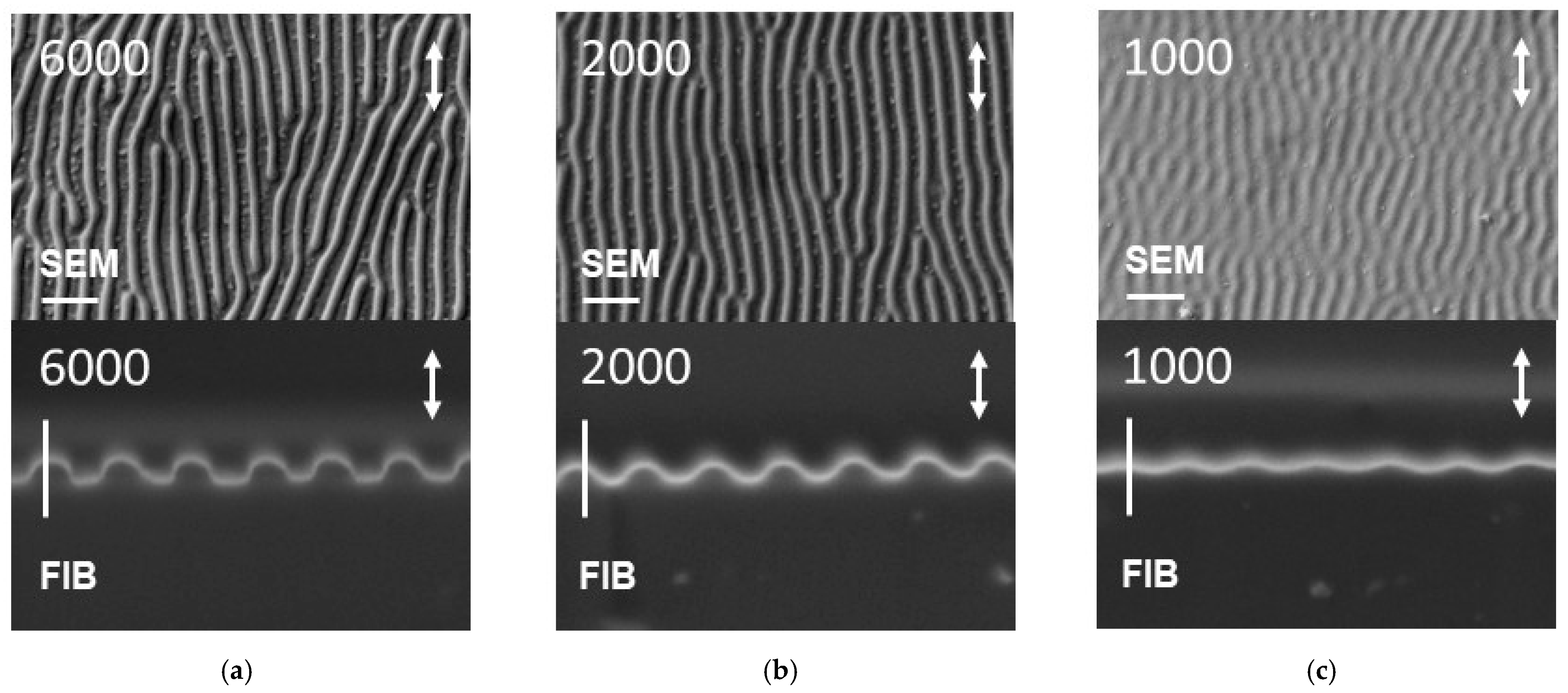
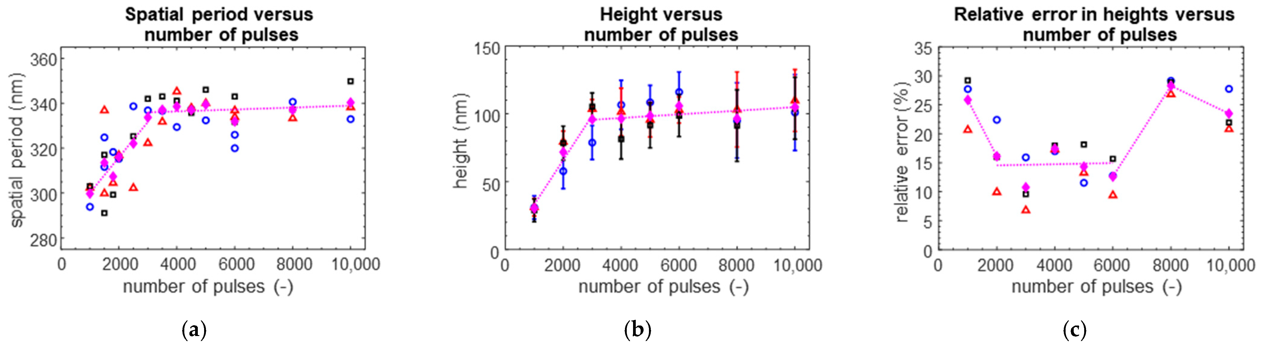
3.1.2. Change with the Pulse Number

We studied the effect of the pulse number on the spatial periods and the heights of the ripples using SEM images and FIB cuts (Figure 6). During this study, we maintained an angle of incidence of θ = 30° of the linearly polarized light, a fluence ϕ of about 4.2 to 4.5 mJ/cm2, and a pulse repetition rate of ν = 10 Hz. Figure 6 depicts exemplary SEM images (top) and FIB cuts (bottom) at (a) 6000 pulses, (b) 2000 pulses, and (c) 1000 pulses. The FIB cuts show that the height of ripples increased with increasing pulse number and that the shapes of the ripples changed; first, they were sinusoidal, and at higher pulse numbers, they became more and more rectangular. We evaluated SEM images and FIB cuts at three positions on each sample, and even at six positions for N = 1500 and N = 6000 (Figure 7). Robust fits through the mean values serve to guide the eyes and were computed in Matlab R2022b (The MathWorks, Inc., Natick, MA, USA). The graphs indicate that an increase in the pulse number resulted in a moderate, approximately linear increase in the spatial periods up to about 3000 pulses (Figure 7a). Then, they stayed constant until the highest tested value of 10,000 pulses. Similarly, the heights of the ripples rose approximately linearly with increasing number of pulses (Figure 7b). They were also approximately constant from 3000 pulses on. The increase was steeper than the increase in the spatial periods. The relative errors of the heights were high at low pulse numbers (about 25%), then dropped to about 15% at higher pulse numbers, and then rose again (to about 25%) at 8000 and 10,000 pulses (Figure 7c). From all tested pulse numbers, 5000, and especially 3000 and 6000 pulses, resulted in the most homogeneous heights with the least relative errors, while simultaneously, the mean spatial periods and heights had reached their saturation values. Both the spatial periods and the heights did not significantly differ from those of the sample fabricated with a slightly higher fluence of about 5.7 to 6.2 mJ/cm2 with θ = 30° (see Section 3.1.1).

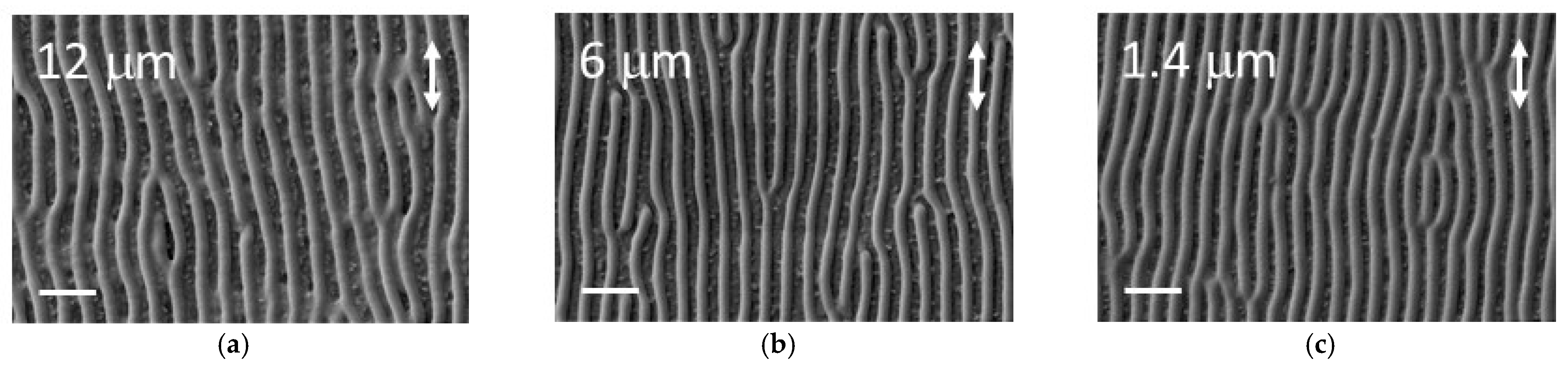
3.1.3. LIPSS on Ultrathin PET Foils

We succeeded in the formation of LIPSS on ultrathin PET foils by using a carrier substrate (Figure 8 and Table 1). For all samples, N = 6000 pulses of linearly polarized light, an angle of incidence of θ = 30°, and a pulse repetition rate of ν = 10 Hz were applied. We used two average fluence values, namely ϕ of about 4.2 to 4.5 mJ/cm2 and ϕ of about 5.7 to 6.2 mJ/cm2. The mean spatial periods Λ ± standard deviations were evaluated at three and five exemplary positions, respectively, on the ultrathin foils and the 50 μm thick reference foil (Table 1).
For both fluences, the spatial periods slightly increased with increasing foil thickness t for the ultrathin foils with t = 1.4 μm, 6 μm, and 12 μm. This change was not significant when thicknesses of 1.4 μm and 6 μm were compared for the lower fluence value; all other changes were greater than the computed standard deviations. However, for the reference foil with a thickness of 50 μm, the spatial period decreased again. A slightly higher fluence value ϕ of about 5.7 to 6.2 mJ/cm2 led to a significant decrease in the spatial periods compared to the lower value of about 4.2 to 4.5 mJ/cm2. In the last column of Table 1, the formulas of the corresponding linear trend lines through the mean values are shown. They were computed in Microsoft Excel (Microsoft Office LTSC Professional Plus 2021, Microsoft Corporation, Redmond, WA, USA).

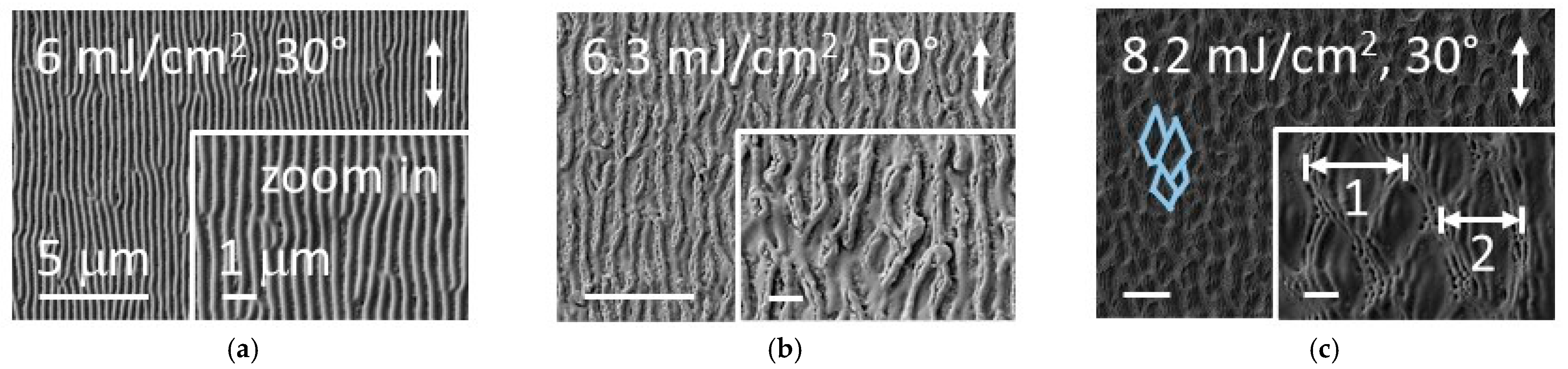
3.1.4. Changes Due to an Increase in Fluence

The ripples on the reference samples fabricated with the slightly higher fluence of ϕ = 5.7 to 6.2 mJ/cm2 appeared to extend longer in the lateral direction parallel to the direction of polarization than those fabricated with ϕ = 4.2 to 4.5 mJ/cm2 (Figure 9). Furthermore, they showed a more distinct preferential direction and therefore a higher order, i.e., they arranged more uniformly along the direction of the polarization. We have repeatedly monitored the homogeneity of the LIPSS on these foils by SEM imaging at five different evenly distributed positions on the laser-processed area and found them to have a very similar morphology at all positions. This is emphasized by the low relative standard deviations of about 2% of the spatial periods (Table 1).
Next, we studied the influence of an increase in fluence on the nanoripples’ morphology compared to the so-far used higher reference value of ϕ = 5.7 to 6.2 mJ/cm2 (i.e., a pulse energy E = 12 mJ) (Figure 10a). For all samples, N = 6000 pulses of linearly polarized light, an angle of incidence of either θ = 30° or θ = 50° and a pulse repetition rate of ν = 10 Hz were applied. An increase in the pulse energy E and therefore in the fluence ϕ to, respectively, 20 mJ and 6.3 mJ/cm2 led to the generation of two finer ripples on top of the base ripples (Figure 10b)—one peak split up into two separate ones. The higher the fluence became, the more fine ripples were generated and the more the ripples lost their parallelism (Figure 10c). Some of the fine ripples disconnected and became dots. At about 8.2 mJ/cm2 (i.e., a pulse energy E = 16 mJ), the structures resembled “diamonds” because the finer ripples as well as the dots enclosed diamond-shaped areas without ripples. In Figure 10c exemplary diamond-shaped structures are highlighted by light blue lines. The tops of their walls were furnished with several fine ripples and dots that were connected at some positions. The maximum width of the diamonds was 2.25 μm ± 0.48 μm (±21%, n = 20) in the direction perpendicular to the polarization. Exemplary measurement data in the inset of Figure 10c explain how the maximum width was determined. The distance between the fine ripples was approximately 0.247 ± 0.069 μm (±28%, n = 20).

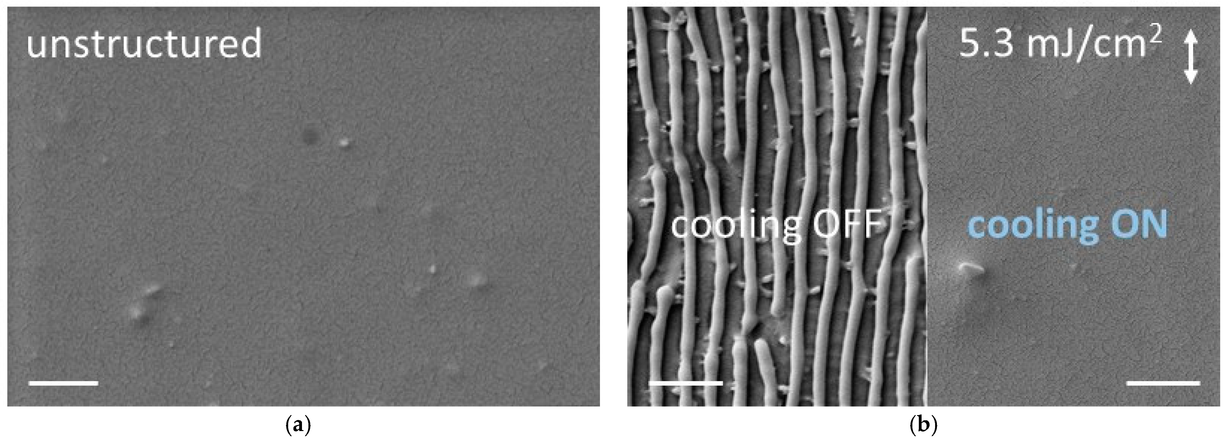
3.1.5. Change in Ripple Morphology Due to Substrate Cooling and a Water Layer

Cooling of the PET foil with a Peltier element below 0 °C to between −1.5 °C and −2 °C (±1 °C) caused the nanoripples either to vanish completely in the case of a fluence value of ϕ = 5.3 mJ/cm2 (Figure 11) or to fade and to become very short in the case of a slightly higher fluence value of ϕ = 5.7 to 6.2 mJ/cm2. At a critical temperature of approximately 2.4 °C (±1 °C), some iridescent ripples formed again when the lower aforementioned fluence value was chosen, at which they had completely vanished at a cooling temperature of between −1.5 °C and −2 °C (±1 °C). For all the laser-processed samples N = 6000 pulses, an angle of incidence of θ = 30° and a pulse repetition rate of ν = 10 Hz were applied. Briefly before and during processing, water droplets condensed on the PET foil from ambient air. They expanded into a thin water film on the processed area during laser fabrication because it had changed the contact angle of PET. The amount of condensed water depended on the relative humidity of the ambient air. Preliminary contact angle measurements using a custom-tailored setup, 1 μL droplets of deionized water, and the θ/2 method for evaluation gave a reduction of the contact angle from ~76° (±3°, n = 12) on the pristine PET foil to ~48° (±2°, n = 3) on an example laser-processed area, where ripple formation had been suppressed by cooling.
Putting a water layer with a thickness of 7.9 mm in front of the PET during laser processing using a customized sample holder (Figure 12a) led to more irregular ripples compared to the reference sample fabricated in the air (Figure 12b), and furthermore to the generation of craters. The specifically designed rotatable sample holder allowed for the usage of an angle of incidence of θ = 30°. Here, N = 6000 pulses, a fluence Φ of 5.7 to 6.2 mJ/cm2, and a pulse repetition rate of ν = 10 Hz were applied. The peak-to-peak distances in between the ripples were reduced from dpp,air = 351 nm ± 29 nm (±9%, n = 150) to dpp,water = 292 nm ± 43 nm (±15%, n = 153). The decrease in the mean peak-to-peak distance of ~−17% was not significant. For the fabrication of this kind of irregular nanoripples, the thickness of the water layer was crucial. For smaller thicknesses of the water layer, such as 6 mm, the ripples faded, and for even smaller thicknesses of 4 mm or 2 mm, the processed areas became more and more inhomogeneous.

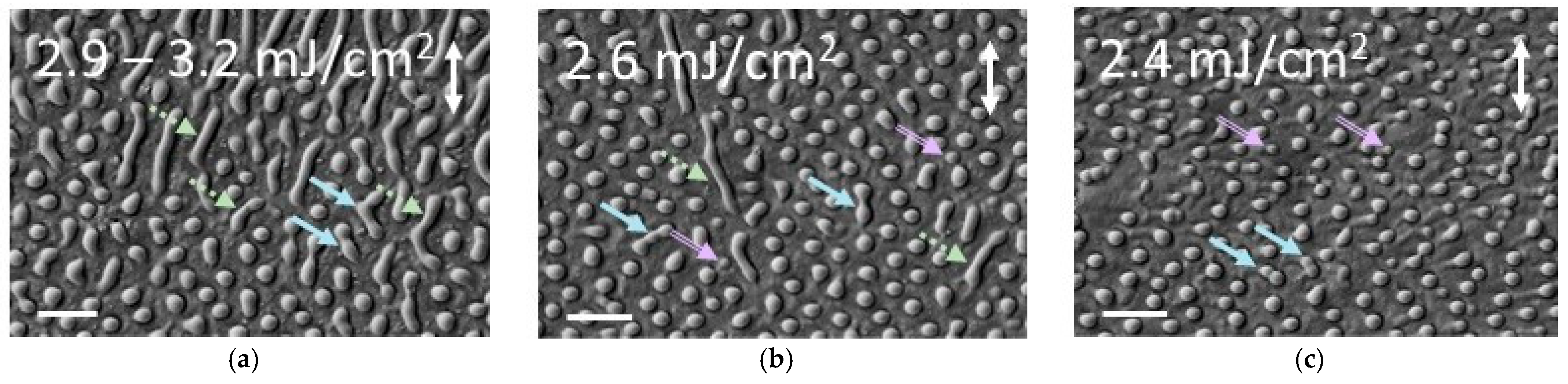
3.2. Nanodots Due to a Decrease in Fluence

Before we had discussed that a decrease in the fluence led to shorter ripples concerning their lateral extension along the direction of the linear polarization (Figure 9). A further reduction in the fluence gave rise to even shorter ripples and the generation of nanodots (Figure 13). Here, the nanodots were distributed randomly. All samples were fabricated using linearly polarized light with an angle of incidence of θ = 40°, applying N = 6000 pulses with a pulse repetition rate of ν = 10 Hz. As the fluence values were decreased from ϕ = 2.9 mJ/cm2–3.2 mJ/cm2 (Figure 13a), i.e., pulse energies E of approx. 7.5 mJ–8 mJ, to ϕ = 2.6 mJ/cm2 (Figure 13b), i.e., pulse energies E of approx. 6.5 mJ, the proportion of the short ripples became less. At ϕ = 2.4 mJ/cm2 (Figure 13c), i.e., pulse energies E of approx. 6 mJ, mainly nanodots were left.
It seems that at least some nanoripples in Figure 13a,b had been formed from merged nanodots whose shapes are still visible (see exemplary ripples marked by solid light blue arrows). The short ripples aligned preferentially in the direction of polarization. Most of them are arranged not perfectly in parallel to the polarization vector (see exemplary ripples marked by dotted light green arrows). Some dots are very short and have a considerably smaller diameter than the others (see exemplary dots marked by double-lined light magenta arrows); they might constitute nucleation centers for nanodot formation. The dots’ mean equivalent disc radii ± standard deviations are 129 nm ± 35 nm (±27%, n = 80) for Figure 13a, 115 nm ± 30 nm (±26%, n = 100) for Figure 13b, and 106 nm ± 15 nm (±15%, n = 100) for Figure 13c, i.e., the mean radii decreased with decreasing fluence, although not significantly. Furthermore, the dots’ radii became more homogeneous when less energy was used, which is reflected by the decreasing relative standard deviations. The dots’ centers are located at distances of 441 nm ± 90 nm (±20%, n = 50) for Figure 13a, 391 nm ± 49 nm (±12%, n = 100) for Figure 13b and 339 nm ± 58 nm (±17%, n = 100) for Figure 13c from the centers of their nearest neighbors, i.e., the dots moved closer together when the fluences decreased, although not significantly. The mean height of the dots ± standard deviations measured in FIB cuts was 96 nm ± 26 nm (±38%, n = 23); here, the dots were cut at an arbitrary position that was not necessarily the highest one. However, it has to be noted that the dots were far more sensitive to variations in the fluence than the ripples, wherefore they were not as homogeneously distributed over the cm2-sized sample area due to slight variations in the laser beam energy over the area. Thus, the approx. same spots on the laser-processed areas were analyzed for each set of parameters.

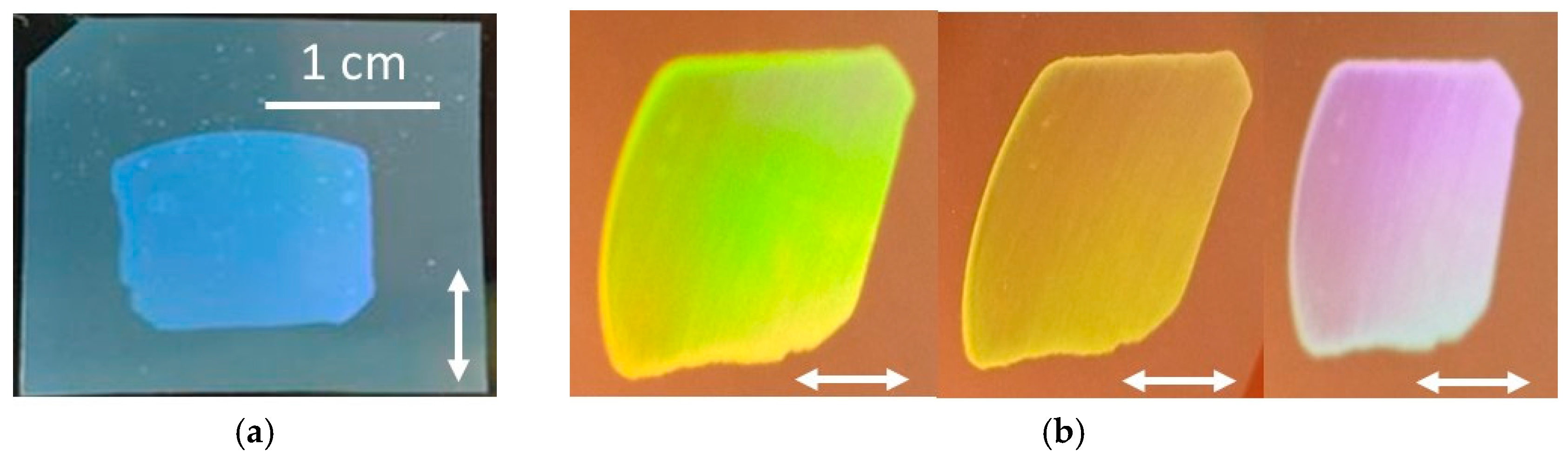
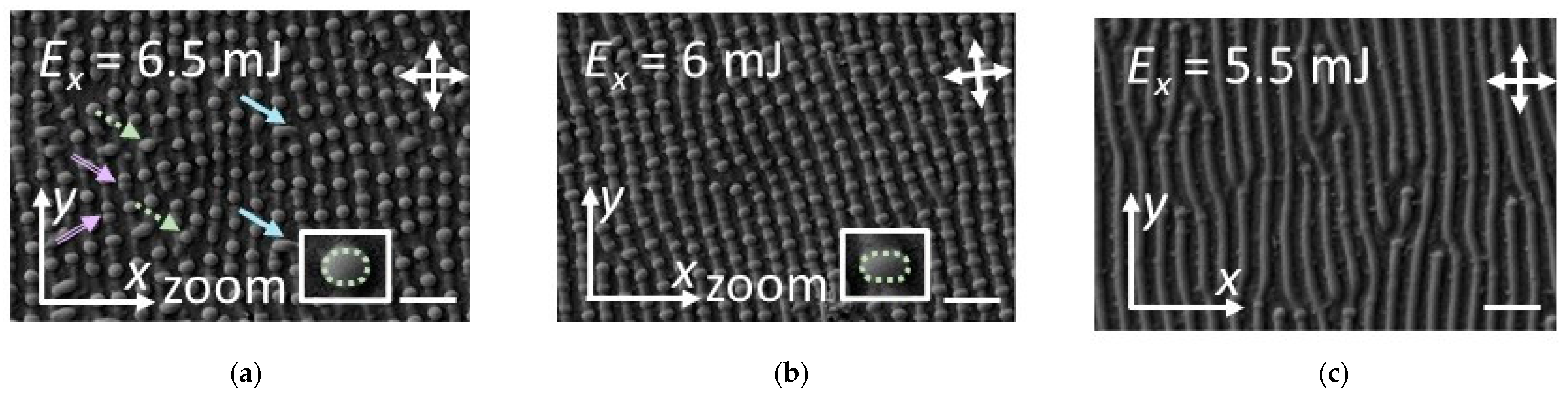
3.3. Nanoscale Grids and Hierarchical Structures Due to Superposition of Two Polarization Directions

In some cases, superimposing two different directions of linear polarization increased the complexity of the structures (Figure 14 and Figure 15). To this end, we performed two successive steps applying two directions of polarization perpendicular to each other employing θ = 30° and ν = 10 Hz for all samples. First, we used laser light with a linear polarization in the y-direction, and then—in a second step—we continued with light linearly polarized in the x-direction. For further details, the reader is referred to Section 2.1.3.
The number Ny and the energy Ey of the pulses with the polarization in the y-direction were kept constant at Ny = 6000 and at Ey = ~12–12.5 mJ (i.e., at ϕ = ~6–6.3 mJ/cm2). The energy Ex of the pulses with the polarization in the x-direction was kept constant at Ex = ~12–12.5 mJ (i.e., at ϕ = ~6–6.3 mJ/cm2). The influence of a decrease in the pulse number Nx of the second polarization direction was investigated (Figure 14). Using Nx = 6000 (Figure 14a) or Nx = 4000 pulses the first layer of ripples along the y-direction was completely erased and overwritten. For Nx = 6000 pulses the ripples of the second layer looked well defined. However, they merged and bifurcated at some positions, which made it difficult to evaluate the spatial period by Fourier transformation from the low number of ripples shown in Figure 14a; the corresponding spatial period was 349 nm ± 6 nm (±2%, n = 3). In contrast, for Nx = 4000 pulses, the ripples appeared a bit washed out, i.e., maybe the formation of defined ripples was hindered by the first layer of ripples. Their spatial period was 331 nm ± 6 nm (±2%, n = 3), i.e., the same as for the single layers shown in Figure 6a, Figure 7a and Figure 9. The situation changed completely when we used considerably lower pulse numbers in the second direction, namely either Nx = 2000 (Figure 14b), Nx = 1500, or Nx = 1000 (Figure 14c). In this case, the second layer of ripples only partly overwrote the first one, and nanogrids formed. In the cases of Nx = 1500 and Nx = 1000, the nanogrids were more defined and homogeneous than for Nx = 2000 across the whole cm2-sized processed area. Evaluating the grid constants in the two directions of polarization, i.e., the spatial periods, via 2D FFT of SEM images like those in Figure 14 resulted in Λx = 332 nm ± 11 nm (±3.4%, n = 3) and Λy = 332 nm ± 4 nm (±1.2%, n = 3) for Nx = 2000, Λx = 336 nm ± 12 nm (±3.6%, n = 3) and Λy = 325 nm ± 8 nm (±2.5%, n = 2 due to bad quality at one position) for Nx = 1500, and Λx = 314 nm ± 12 nm (±3.7%, n = 3) and Λy = 343 nm ± 8 nm (±2.3%, n = 3) for Nx = 1000. This means that the spatial periods in both directions and therefore the grid constants were in the same range as those listed in Table 1 and shown in Figure 7a for θ = 30° and different energies and pulse numbers.
The energy used for ripple generation was then set to a lower fixed value in the first direction of polarization and gradually reduced in the second direction of polarization (Figure 15). The resulting formations resembled pearl chains. As before, the number Ny and the energy Ey of the pulses with the polarization in the y-direction were kept constant, this time at Ny = 6000 and Ey =~8.5 mJ (i.e., at ϕ = ~4.2–4.3 mJ/cm2). The energy Ex of the pulses with polarization in the x-direction was considerably reduced to Ex = ~6.5 mJ (i.e., ~3.2–3.3 mJ/cm2) (Figure 15a), Ex = ~6 mJ (i.e., ~3 mJ/cm2) (Figure 15b), and Ex = ~5.5 mJ (i.e., ~2.7–2.8 mJ/cm2) (Figure 15c), respectively, to trigger the formation of nanodots. Values in this energy range have also been used to create only nanodots, which are shown in Figure 13. This resulted in ripples with regularly distributed nanodots on their tops (Figure 15a,b) or at their beginnings and ends (Figure 15c). For the highest tested energy Ex = ~6.5 mJ, sometimes merged dots bridged two ripples (light blue arrows) and seldomly two dots touched because they originated very closely to each other (double-lined light magenta arrows); sometimes dots were located in between the ripples and not on their tops (dashed light blue arrows). Reducing the energy in the second direction of polarization (Figure 15b) the dots’ shapes became more elliptical with the minor axis being parallel to the ripples and the major axis being aligned along their widths. Furthermore, the ripples appeared to become higher and the dots shorter.
The distances between the dots and their nearest neighbors on the same ripple are 447 nm ± 82 nm (±18%, n = 100) for Figure 15a and 409 nm ± 102 nm (±25%, n = 100) for Figure 15b, i.e., that the dots moved closer together when the energy was reduced; however, the change was not significant, most probably since not all dots on top of the ripples were fully developed. For the lowest energy, the dots formed mainly at the beginnings and ends of the ripples (Figure 15c), and therefore their distances were significantly larger, namely 1500 nm ± 670 nm (±45%, n = 10). The distances between the dots and their nearest neighbors on another ripple were 373 nm ± 64 nm (±17%, n = 100) for Figure 15a, 351 nm ± 36 nm (±10%, n = 100) for Figure 15b, and 628 nm ± 363 nm (±58%, n = 17) for Figure 15c, i.e., taking into account the high standard deviations, they were all within the same range, although their means showed the same qualitative behavior as before. Interestingly, the equivalent disc radii of the dots were 113 ± 13 nm (±11%, n = 100) for Figure 15a, 104 ± 12 nm (±12%, n = 100) for Figure 15b, and, respectively, 93.7 nm ± 5.0 nm (±5%, n = 24) for Figure 15c. The means decreased, however, at first, not significantly. Computing the distances in between the ripples by 2D FFT resulted in spatial periods of 339 nm ± 4 nm (±1%, n = 3) for Figure 15a, 326 nm ± 10 nm (±3%, n = 3) for Figure 15b, and 337 nm ± 11 nm (±3%, n = 3) for Figure 15c. These values are similar to those obtained for ripples with the same set of parameters as used for the first polarization direction (see Figure 6a and Figure 7a and Table 1). Therefore, the second direction of polarization did not influence the ripples’ spatial periods.

4. Discussion

4.1. Nanoripples

Formation of regular nanometric LIPSS requires polarization of the laser light [19,31]. We were able to fabricate irregular nanoripples without a polarizer in the beam path, possibly due to the attenuator and the dielectric mirror polarizing the unpolarized laser light to some extent. On 50 μm thick PET foils, we measured the heights of regular nanoripples with spatial periods from ~214 nm to ~613 nm, as well as of irregular ones, and assessed their shapes using FIB cuts (Figure 3 and Figure 4). This resulted in measurement values systematically higher than those obtained from AFM topography images in [24,25,26,27,32], although the processing parameters and used materials were very similar or even the same. Probably, the differences are caused—to some extent—by tip-sample convolution, which is typical of AFM measurements, especially in the case of high densely packed ripples with steep slopes such as ours. Therefore, the valleys in between the ripples might not be reached—an effect which was described in [5]. Furthermore, some of the literature values for ripple heights h were calculated from the arithmetic mean roughness or average roughness Ra of recorded AFM topography images—using the relation h = 2Ra. The average roughness accounts for the arithmetic average of profile height deviations from the mean line. This software-aided method is fast and easy to compile. For the two following reasons, this method might deviate from the true peak-to-valley heights of the ripples. First, the shapes of the ripples influence the outcome: only in the case of ripples of nearly rectangular shape (i.e., in our case, the use of high pulse numbers, see Figure 6) will the results of the two calculation methods match. Second, analyzing the AFM topographies shown in [24,25,27,32] reveals that the ripples’ shapes from AFM data appear systematically wider compared to those assessed by FIB cuts—most probably due to tip-sample convolution.
Shapes and mean ripple heights depended on the angle of incidence (Figure 3 and Figure 4). Given the high absolute and relative standard deviations, very few heights differed significantly, e.g., ripples fabricated with θ = 30° were significantly higher than those fabricated with θ = 10° and θ = 20°. The most extreme values represented by the whiskers revealed the large variability of possible height values. Ripple merging and bifurcation caused extreme variations in ripple heights, namely exceptionally short and high ripples (Figure 3a). Regularity depended on the angle of incidence and was most pronounced at θ = 20° and θ = 30° with relative standard deviations between 9% and 23% compared to 31–49% for the other angles of incidence. The underlying cause of the relation between nanoripple regularity and angle of incidence remains unknown. However, it may be connected to the surface roughness of the pristine PET foils: Csete et al. [51] reported that perfectly flat spin-coated PC films upon 193 nm—ArF excimer laser processing led to more regular LIPSS compared to commercial PC foils. In cases of applications that require very precise geometries, other methods such as direct laser interference patterning (DLIP) [52,53] and electron [54] or ion beam lithography [55] are indispensable because the LIPSS formation process lacks the necessary regularity control feature.
Some of the nanorippled PET surfaces showed iridescence (Figure 5). Iridescence, i.e., the angle of view or the angle of illumination changes the color appearance of a certain surface, is an example of a structural coloration mechanism that is also observed in nature [10]. Here, it is thought to arise from diffraction gratings formed by the nanoripples themselves such as in the iridescent fan of the seed-shrimp (ostracod crustacean) Azygocypridina lowryi [56]: a similar color spectrum is observed, which is in this case caused by ripples with peak-to-peak distances in the range of 480 nm to 550 nm. A similar effect was also achieved by laser-induced ripples on metals such as aluminum [57] and copper [58]. In [57], ripples with a spatial period of 540 nm rendered aluminum iridescent, while in [58], nanoripples on copper with spatial periods between 600 nm and 665 nm caused the copper´s color to change with the angle of view. All the ripple distances of the above-cited works [56,57,58] are therefore within the range of the nanoripples we fabricated. For this kind of low-energy color change mechanism, no chemical energy is needed, which might be an advantage in the biological evolution of certain species, e.g., of the seed-shrimp Azygocypridina lowryi [56], and also for long-term stability, as these colors do not fade like pigment colors [10]. This might be desirable for applications in communication, decoration, and anti-counterfeiting design [10].
A water layer with a thickness of 7.9 mm before the sample decreased the mean peak-to-peak distances between the ripples on 50 μm thick PET foils (Figure 12), although not significantly. This is most probably due to the higher refractive index of water of 1.36 at 248 nm and 25 °C [59] compared to air, which then changes the effective refractive index neff. According to Equation (1), this higher effective refractive index neff reduces the spatial periods. The purpose of the water layer was to increase the effective refractive index neff, thus adding another tuning parameter for the spatial period Λ to the system. In addition to neff, the angle of incidence θ can be adjusted. Similarly, the spatial periods diminished by several times, when LIPSS on metals were produced by a femtosecond laser in liquid environments instead of air [60]. Interestingly, a water film that was generated by melting a thin frost layer on the target silicon surface not only increased the quality of laser-ablated microstructures considerably but also gave rise to high-spatial-frequency LIPSS [61]. These were not generated at all without the frost layer, even when the same processing parameters had been applied.
Our nanoripples fabricated with a water layer in front of the PET were not as regular as the ones fabricated in the air and occasionally craters appeared. Applying thinner water layers led to faded ripples (in case of 6 mm) or to very inhomogeneous surfaces with a few faded ripples at some positions (in case of 4 mm and 2 mm). This is most probably due to bubbles generated either in between the fused-silica plate and the polymer foil or at their interfaces. Some mechanisms of bubble generation and their effects on the beam path were described in [36]. In the following, we discuss them concerning our experimental configuration. Bubbles might not have been able to escape easily from the sample holder in case the water layer was too thin: it seems likely that they adhered either to the fused-silica plate or to the PET foil. These bubbles are thought to have diverged the—in our case—nearly parallel laser light (after the telescope configuration of the lenses) since the refractive index of water is higher than the one of water vapor; others might have collapsed and caused a flow field therein. Furthermore, cooling of the PET surface by the water layer may have affected structure formation [37].
Previously, slightly different processing parameters of KrF excimer laser treatment of PET using an approx. 5 mm thick water layer and θ = 0° resulted in worm-like structures [35]. Only in exceptional cases several ripples were visible, namely at the lowest fluence of 8 mJ/cm2 at very low and high operating voltages. At fluences above the ablation threshold, porous structures formed [62]. In water the ablation threshold of PET was found to be less than half of that in air, namely 14 mJ/cm2 compared to 29 mJ/cm2 [62]; these values were determined for a 75 μm thick PET foil from Mylar by using a similar ns KrF excimer laser setup [62]. This low ablation threshold value together with fewer bubbles deviating the laser beam might explain why we generated nanoripples instead of worm-like structures at a lower fluence value together with a thicker water layer of 7.9 mm compared to the 5 mm in [35]. Also, for ns excimer laser treatment of PS in air, a similar trend was observed [63]: the formation of nanoripples and worm-like structures at lower and higher fluences, respectively.
We succeeded in suppressing ripple formation on 50 μm thick PET foils by substrate cooling (Figure 11). This cannot be discussed without considering the water layer formed during cooling. However, it has to be pointed out that the thickness of the water film increased with the relative humidity of the ambient air; it was very thin, probably not continuous, and barely visible at low relative humidity, and very pronounced at high relative humidity. First, droplets condensed on the PET foil from the surrounding air. Then, they expanded to form a water film in response to a lower contact angle due to laser-processing. Due to gravity, the water layer was thicker at the bottom than at the top in case it was continuous. The initial droplets might have served as plano-convex lenses focusing the laser beam for physicochemical surface modification. Then, the water layer formed due to physicochemically induced contact angle reduction. Bubbles might have escaped the film readily because of an open interface to the surroundings and such might not have diverged the laser beam. Therefore, we assume substrate cooling to interfere with the temperature field. As ripple generation has been suppressed, this result might be considered experimental evidence that the temperature field is the positive feedback mechanism needed for structure formation, as described in [22,28,64]. Interestingly, cooling of the target silicon surface in [61] had the contrary effect and gave rise to high-spatial-frequency LIPSS. In the future, interesting follow-up experiments would include high-speed camera recording of bubble generation during laser processing, water temperature measurements, physicochemical analysis of the liquid after laser irradiation, and nanostructure analysis upon substrate cooling at various temperatures. Future control of the relative humidity of the ambient air might constitute a way to regulate the existence and thickness of the water layer generated by substrate cooling during laser processing. Multiphysics simulation of the underlying effects is challenging but would provide a way for future structure prediction.
We fabricated nanoripples on ultrathin foils with thicknesses of 1.4 μm, 6 μm, and 12 μm (Figure 8). In the future, these foils might be possibly applied to improve the efficiency of ultrathin solar cells [65] by using the principle described in [66]. Or, they might cover arbitrarily shaped objects with nanoripples to equip them with bacteria repellency [32] or antiadhesion against nanofibers [4,5]. We found different thinner foil thicknesses t to result either in ripples of significantly higher (t = 12 μm), smaller (t = 1.4 μm), or the same (t = 6 μm) spatial periods compared to the 50 μm thick reference foil depending on the applied fluence. This is in accordance with previous work [22], where the thickness of PS films, the applied fluence, and the thermal and optical properties of the underlying substrate affected LIPSS generation. According to the theoretical considerations presented in [22], these parameters influenced the temperature of the material during processing. However, the tested film thicknesses in [22] were about one magnitude of order smaller than the ones in our case, namely some hundreds of nanometers compared to some microns. Provided that the trend described in Figure 3 of [22], with an initial increase, a plateau, and then a decrease in spatial periods and heights with increasing film thickness, is also applicable in our case, then the film thicknesses of several microns we used represent the initial slope of the curve.
Our FIB cuts revealed that the ripple shape changed with the pulse numbers (Figure 6). At lower values, they were approximately sinusoidal, and at higher ones, they became increasingly rectangular. Our results indicate that both the height and spatial period of the ripples increased with increasing number of pulses and then reached a saturation value at ~3000 pulses (Figure 7). The slopes are approximately linear. This effect could be exploited to increase the mean ripple height from ~25 nm to ~100 nm (i.e., by ~300%) by using higher pulse numbers. The spatial period would increase by only ~12%, and this moderate change could be balanced by using slightly lower angles of incidence (see Equation (1)). The ripple heights measured differed slightly depending on the measurement position on the processed surface, which may have been caused by slightly inhomogeneous fluences over the several square centimeter-sized processed areas as a consequence of a non-uniform laser profile. Masks could be used to restrict the processed area and guarantee a defined fluence. For very low and high pulse numbers, the relative variations in height increased, which means that the regularity of the ripples decreased. The trends in height and spatial period observed also match those described by Rebollar et al. [67] for femtosecond laser-induced LIPSS on polymer films (including PET). LIPSS from ns UV laser processing, in contrast, were reported to first generate nanorough surfaces with several randomly located nanodot-like surface features of various sizes [14,22,64]. However, Rebollar et al. [28] calculated the temperature increase induced by laser irradiation, which indicates that LIPSS formation in amorphous spin-coated polymer films takes place by devitrification of the film surface at temperatures above the characteristic glass transition temperature Tg of the polymers. With the parameters we chose for our study of the influence of pulse number, we did not observe an initial regime with distinct nanodot formation. These differences in the structures observed and in the different pulse numbers needed for LIPSS formation on the same polymer make it clear that, currently, each combination of material, substrate, and setup requires its own procedure to optimize LIPSS quality.
When we increased the fluence, the ripples became longer and parallel to the linear polarization (Figure 9). Above a certain threshold, they separated into finer ripples (Figure 10b). This process started with twin peaks at approx. 6.3 mJ/cm2 and then led to diamond-shaped surface features at about 8.2 mJ/cm2 (Figure 10c). These structures can be considered hierarchical: the tops of the diamonds’ walls exhibited several finer ripples and nanodots, both of which were connected at some positions. It seems likely that—given a proper theoretical explanation of the self-assembly mechanism of these diamond-like structures—their regularity might be improved in the future.

4.2. Nanodots Due to a Decrease in Fluence

We succeeded in forming about 96 nm high nanodots on PET foils at low fluences in the range of 2.4–3.2 mJ/cm2, using linearly polarized laser light (Figure 13). Their mean equivalent disc radii (~106 nm to ~129 nm) and their mean center-to-center distances (~339 nm to ~441 nm) increased slightly with increasing fluence. At the lowest fluence value, only dots were present, while at the higher values, some dots merged into short ripples. This is in agreement with the work of Csete and Bor [64] who patterned PET using mainly a 193 nm—ns ArF excimer laser. They showed experimentally that with this specific setup, proliferating nanogranules constituted the points of origin for ripple formation. Interestingly, using other parameters, we did not observe nanogranules on the surface before ripple formation (Figure 6). This could mean that there are two different ripple formation mechanisms at lower and higher fluences, respectively, which might also influence the parallel orientation of the resulting nanoripples (Figure 9). For our surface nanodots on PET, we envision a possible future application in biomimetics. As mentioned in Section 1, surface nanoripples on PET bioinspired by the calamistra of cribellate spiders reduced the adhesion of nanofibers [4,5] and bacteria [32]. However, the calamistra of some spider species such as Amaurobius similis and Menneus superciliosus not only possess surface nanoripples but also protrusions that look more like nanodots or nanospikes [4]. Their role is still elusive and might be probably unraveled with the help of biomimetic nanodots of similar dimensions. A promising candidate for a further future application area is plasmonics [68]. Covering the foils with thin layers of gold or silver, the nanodots might couple photons into surface plasmon polaritons. In [24,40], separate gold nanowires were fabricated with the help of LIPSS on PET, which had partly shielded the surface during thermal vacuum evaporation under an angle. They showed surface plasmon resonances. Similarly, separate gold or silver nanodots for the generation of localized surface plasmons might be produced using the PET surface nanodots that we fabricated in this work.
Rebollar et al. [29] fabricated densely packed nanodots with center distances similar to those of ours on PET surfaces by applying circularly polarized ns UV laser light. Csete et al. [51] observed the beginning transformation of line-shaped structures into droplets below a particular thickness of spin-coated PC films on a glass substrate processed by polarized ArF excimer laser light. This was explained by laser-induced melting across the whole film thickness and subsequent de-wetting of the substrate. We assume that a similar mechanism might be involved in the formation of the nanodots presented in this work: semi-crystalline PET might melt (in the case of the crystalline phase of PET) or rearrange (in the case of the amorphous phase of PET) preferentially at nanograins (e.g., filler particles) or other structural inhomogeneities on the surface and in the top layer of the foil. We found evidence for such inhomogeneities in SEM images (Figure 11a) and optical microscope images. These inhomogeneities might serve as seeds for nanodot formation as they might become covered by rearranged or melted material and thus concentrate PET around and on them. Cui et al. [22] observed the replacement of ripple formation by distorted LIPSS with drop-like structures on spin-coated PS films of intermediate thickness on silicon. These publications suggest that the interplay between material thickness, substrate, and laser parameters is decisive in the mechanism that leads to the formation of surface nanodots. High-fluence ns KrF excimer laser processing resulted in extremely densely packed nanodots on 50 μm thick polyethersulphone foils [69], while ours are in most cases separated and their surfaces do not touch each other; polyethersulphone formed LIPSS at similar fluences and pulse numbers as the PET foils used in this study. In contrast to our randomly arranged nanodots, highly regular hexagonally arranged nanodot-like surface protrusions were created by Porta-Velilla et al. [70] on nickel tungsten alloy tapes using picosecond UV laser pulses. These protrusions were ~200 nm in diameter, ~130 nm high, and exhibited closest-neighbor distances of ~400 nm.

4.3. Nanoscale Grids and Hierarchical Structures Due to Superposition of Two Polarization Directions

We produced nanogrids (Figure 14) and hierarchical structures that exhibited nanoripples with nanodots on their tops—formations that resembled pearl chains (Figure 15). To this end, we successively superimposed two linearly polarized laser beams by rotating the sample by 90°, rendering the directions of polarization perpendicular to each other. We found that the grid constants were in the same range as the spatial periods of nanoripples fabricated with similar pulse numbers and fluences. Note that for nanogrids to be generated, the number of pulses in the second direction (2000 or 1000 pulses) needed to be significantly lower than that in the first direction (6000 pulses), while all other parameters remained constant, as otherwise the first structure was completely overwritten. This overwriting might be used to one’s advantage to cover larger areas seamlessly by stitching them together. A similar technique was applied by Csete et al. [51], who used polarized ArF excimer laser light to form a nanogrid on 78 nm thick spin-coated PS film on glass. However, they used 1000 laser pulses in both polarization directions. Nanogrids might be applicable for the formation of regularly spaced separate noble metal nanodots for plasmonics [68] using the technique described in [24]. The walls of the grid are expected to partly shield the surface during thermal vacuum evaporation under an angle. Furthermore, nanogrids with thin layers of gold or silver on top might serve as couplers for the generation of surface plasmon polaritons.
Nanoripples with nanodots on top, resembling pearl chains, formed when we lowered the fluence in the second polarization direction to values used for nanodot generation on flat surfaces. The mean equivalent disc radii (~94 to ~113 nm) and the center-to-center distances of the nanodots (~351 nm to ~447 nm) slightly decreased with decreasing fluence. With decreasing fluence, the nanodots became increasingly elliptical in shape. For the lowest fluence value tested, the nanodots developed mainly at the beginnings and the ends of ripples. Interestingly, the spatial periods of the ripple structures underneath were in the same range as those of single layers of ripples fabricated with the same parameters. Hierarchical structures incorporating LIPSS on polymers have previously been achieved mainly in combination with other techniques for micrometric structure formation, such as DLIP [71] and contact lithography [72].

5. Conclusions

We found ns KrF excimer laser processing to be a versatile technique for achieving various kinds of nanostructures on 50 μm thick PET foil. These ranged from regular nanoripples with spatial periods from ~214 nm to ~613 nm to irregular ripples, nanodots, nanogrids, and hierarchical structures composed of ripples with finer ripples or nanodots on top. Interestingly, we succeeded in forming nanodots when we used very low fluences. In some cases, superimposing two directions of polarization increased the complexity of the structures. This way, we generated nanogrids and “pearl chains”; that is, nanoripples with nanodots on top. To the best of our current knowledge, such kinds of LIPSS structures have not previously been described in the literature. In the case of other parameter combinations, the ripple structures were overwritten, which allows several processed areas to be “stitched” together. Substrate cooling suppressed ripple formation, which could be considered experimental evidence that corroborates theoretical models based on heating by laser pulses [22,28,64]. A water layer of a specific thickness changed ripple morphology, making it more irregular; our custom-built sample holder allowed a water layer to be used also during ripple formation under a certain angle of incidence of the laser beam.
We studied changes in ripple topography upon parameter variation, using SEM images and FIB cuts to fully exclude tip-sample convolution effects that are typically present in AFM images. The angle of incidence of the laser beam determined the spatial periods and heights of the ripples. Some nanoripples showed iridescence. In a beamline without a polarizer, irregular nanoripples formed. The number of pulses influenced the spatial periods, shapes, and heights of the ripples: At pulse numbers below 3000, the spatial periods and the heights decreased approximately linearly. Above this value, both the spatial periods and the heights were saturated. A moderate increase in fluence made the nanoripples longer in the direction parallel to the linear polarization of light and increased their parallelism. An even higher increase in fluence gave rise to hierarchical structures: finer ripples and dots on top of the main nanoripples that were arranged in diamond-like structures. Reducing the PET foil thickness to 12 μm, 6 μm, and 1.4 μm influenced the spatial periods depending on the fluence: they were significantly lower, the same, or higher than the spatial periods of nanoripples on reference foils with a thickness of 50 μm.
We expect that our approaches for structural variability can also be applied to other polymers such as SU-8 [48,49] and PS [24,47] because they develop similar ripple patterns at comparable processing parameters. We foresee numerous possible applications of the structures presented, as—in combination with masks—they allow customized patterning of the surface topography for the antiadhesion of nanofibers [4,5], the repellency of bacteria [32,53], plasmonics [24,40,68] and the alignment and activation of cells [24,29,45,47]. Our experimental achievements will, we hope, inspire theorists to create models that describe the formation of the structures presented here.

Author Contributions

Conceptualization, G.B. and J.H.; methodology, G.B., M.K. and J.H.; software, G.B.; validation, G.B. and M.K.; formal analysis, G.B.; investigation, G.B., M.K. and G.H.; resources, G.B. and J.H.; data curation, G.B.; writing—original draft preparation, G.B.; writing—review and editing, all; visualization, G.B., M.K. and G.H.; supervision, G.B. and J.H.; project administration, G.B. and J.H.; funding acquisition, G.B. and J.H. All authors have read and agreed to the published version of the manuscript.

Funding

This study was in part funded by the European Union’s Horizon 2020 research and innovation programme under the FET Open grant agreement No. 862016 (BioCombs4Nanofibers, http://biocombs4nanofibers.eu (accessed on 13 January 2023)) and in part by the Austrian Science Fund (FWF): T1270-N in the course of the project “Functional Surfaces with Liquid Diode Characteristics”.

Data Availability Statement

Most data are included in this manuscript. More detailed data are available on request from the corresponding author.

Acknowledgments

The authors would like to thank Heide Maria Piglmayer-Brezina (JKU) for SEM characterizations and assistance with the FIB cuts. Many thanks to Martin Kaltenbrunner (JKU) and Florian Hartmann (EPFL) for provision of the PET foils with thicknesses of 12 µm, 6 µm, and 1.4 µm. Furthermore, we thank Alfred Nimmervoll (JKU) for his help with the Peltier element for PET foil cooling, Bernhard Fragner (JKU) for building the rotatable sample holder with the liquid reservoir, and the grammar school student Mia Abermann (BG BRG Gmunden) for her help with data evaluation.

Conflicts of Interest

The authors declare no conflicts of interest.

References

  1. Xiao, G.; He, Y.; Liu, S.; Yi, H.; Du, L. Laser Processing of Micro/Nano Biomimetic Structures. Micro Nano Lett. 2021, 16, 327–335. [Google Scholar] [CrossRef]
  2. Lasagni, A.F.; Alamri, S.; Aguilar-Morales, A.I.; Rößler, F.; Voisiat, B.; Kunze, T. Biomimetic Surface Structuring Using Laser Based Interferometric Methods. Appl. Sci. 2018, 8, 1260. [Google Scholar] [CrossRef]
  3. Hancock, M.J.; Sekeroglu, K.; Demirel, M.C. Bioinspired Directional Surfaces for Adhesion, Wetting and Transport. Adv. Funct. Mater. 2012, 22, 2223–2234. [Google Scholar] [CrossRef] [PubMed]
  4. Buchberger, G.; Meyer, M.; Plamadeala, C.; Weissbach, M.; Hesser, G.; Baumgartner, W.; Heitz, J.; Joel, A.-C. Robustness of Antiadhesion between Nanofibers and Surfaces Covered with Nanoripples of Varying Spatial Period. Front. Ecol. Evol. 2023, 11, 1149051. [Google Scholar] [CrossRef] [PubMed]
  5. Meyer, M.; Buchberger, G.; Heitz, J.; Baiko, D.; Joel, A.C. Ambient Climate Influences Anti-Adhesion between Biomimetic Structured Foil and Nanofibers. Nanomaterials 2021, 11, 3222. [Google Scholar] [CrossRef] [PubMed]
  6. Kirner, S.V.; Hermens, U.; Mimidis, A.; Skoulas, E.; Florian, C.; Hischen, F.; Plamadeala, C.; Baumgartner, W.; Winands, K.; Mescheder, H.; et al. Mimicking Bug-like Surface Structures and Their Fluid Transport Produced by Ultrashort Laser Pulse Irradiation of Steel. Appl. Phys. A 2017, 123, 754. [Google Scholar] [CrossRef]
  7. Zorba, V.; Stratakis, E.; Barberoglou, M.; Spanakis, E.; Tzanetakis, P.; Anastasiadis, S.H.; Fotakis, C. Biomimetic Artificial Surfaces Quantitatively Reproduce the Water Repellency of a Lotus Leaf. Adv. Mater. 2008, 20, 4049–4054. [Google Scholar] [CrossRef]
  8. Liu, Q.; Zhang, J.; Sun, P.; Wang, J.; Zhao, W.; Zhao, G.; Chen, N.; Yang, Y.; Li, L.; He, N.; et al. Achieving Ultralong Directional Liquid Transportation Spontaneously with a High Velocity. J. Mater. Chem. A Mater. 2023, 11, 10164–10173. [Google Scholar] [CrossRef]
  9. Lee, M.; Oh, J.; Lim, H.; Lee, J. Enhanced Liquid Transport on a Highly Scalable, Cost-Effective, and Flexible 3D Topological Liquid Capillary Diode. Adv. Funct. Mater. 2021, 31, 2011288. [Google Scholar] [CrossRef]
  10. Sun, J.; Bhushan, B.; Tong, J. Structural Coloration in Nature. RSC Adv. 2013, 3, 14862–14889. [Google Scholar] [CrossRef]
  11. Liu, Y.; Li, S.; Niu, S.; Cao, X.; Han, Z.; Ren, L. Bio-Inspired Micro-Nano Structured Surface with Structural Color and Anisotropic Wettability on Cu Substrate. Appl. Surf. Sci. 2016, 379, 230–237. [Google Scholar] [CrossRef]
  12. Stratakis, E.; Jeon, H.; Koo, S. Structures for Biomimetic, Fluidic, and Biological Applications. MRS Bull. 2016, 41, 993–1001. [Google Scholar] [CrossRef]
  13. Stoian, R.; Bonse, J. (Eds.) Ultrafast Laser Nanostructuring; Springer Series in Optical Sciences; Springer International Publishing: Cham, Switzerland, 2023; Volume 239, ISBN 978-3-031-14751-7. [Google Scholar]
  14. Rebollar, E.; Castillejo, M.; Ezquerra, T.A. Laser Induced Periodic Surface Structures on Polymer Films: From Fundamentals to Applications. Eur. Polym. J. 2015, 73, 162–174. [Google Scholar] [CrossRef]
  15. Aravind, A.; Jayaraj, M.K.; Kumar, M.; Chandra, R. The Dependence of Structural and Optical Properties of PLD Grown ZnO Films on Ablation Parameters. Appl. Surf. Sci. 2013, 286, 54–60. [Google Scholar] [CrossRef]
  16. Lorusso, A.; Nassisi, V.; Congedo, G.; Lovergine, N.; Velardi, L.; Prete, P. Pulsed Plasma Ion Source to Create Si Nanocrystals in SiO 2 Substrates. Appl. Surf. Sci. 2009, 255, 5401–5404. [Google Scholar] [CrossRef]
  17. Stefan, N.; Mulenko, S.A.; Skoryk, M.A.; Popov, V.M.; Smirnov, A.B. Influence of Hybrid Fe/Cr Parameters Structures Synthesised with Laser Radiation on Their Photosensitivity. J. Mater. Sci. Mater. Electron. 2023, 34, 1830. [Google Scholar] [CrossRef]
  18. Bonse, J.; Hohm, S.; Kirner, S.V.; Rosenfeld, A.; Kruger, J. Laser-Induced Periodic Surface Structures—A Scientific Evergreen. IEEE J. Sel. Top. Quantum Electron. 2017, 23, 9000615. [Google Scholar] [CrossRef]
  19. Bäuerle, D.W. Laser Processing and Chemistry, 4th ed.; Springer: Berlin/Heidelberg, Germany, 2011; ISBN 9783642176128. [Google Scholar]
  20. Bonse, J. Quo Vadis LIPSS?—Recent and Future Trends on Laser-Induced Periodic Surface Structures. Nanomaterials 2020, 10, 1950. [Google Scholar] [CrossRef] [PubMed]
  21. Van Driel, H.M.; Sipe, J.E.; Young, J.F. Laser-Induced Periodic Surface Structure on Solids: A Universal Phenomenon. Phys. Rev. Lett. 1982, 49, 1955–1958. [Google Scholar] [CrossRef]
  22. Cui, J.; Nogales, A.; Ezquerra, T.A.; Rebollar, E. Influence of Substrate and Film Thickness on Polymer LIPSS Formation. Appl. Surf. Sci. 2017, 394, 125–131. [Google Scholar] [CrossRef]
  23. Rodríguez-Beltrán, R.I.; Hernandez, M.; Paszkiewicz, S.; Szymczyk, A.; Rosłaniec, Z.; Ezquerra, T.A.; Castillejo, M.; Moreno, P.; Rebollar, E. Laser Induced Periodic Surface Structures Formation by Nanosecond Laser Irradiation of Poly (Ethylene Terephthalate) Reinforced with Expanded Graphite. Appl. Surf. Sci. 2018, 436, 1193–1199. [Google Scholar] [CrossRef]
  24. Barb, R.A.; Hrelescu, C.; Dong, L.; Heitz, J.; Siegel, J.; Slepicka, P.; Vosmanska, V.; Svorcik, V.; Magnus, B.; Marksteiner, R.; et al. Laser-Induced Periodic Surface Structures on Polymers for Formation of Gold Nanowires and Activation of Human Cells. Appl. Phys. A Mater. Sci. Process 2014, 117, 295–300. [Google Scholar] [CrossRef]
  25. Siegel, J.; Heitz, J.; Švorčík, V. Self-Organized Gold Nanostructures on Laser Patterned PET. Surf. Coat. Technol. 2011, 206, 517–521. [Google Scholar] [CrossRef]
  26. Slepička, P.; Chaloupka, A.; Sajdl, P.; Heitz, J.; Hnatowicz, V.; Švorčík, V. Angle Dependent Laser Nanopatterning of Poly(Ethylene Terephthalate) Surfaces. Appl. Surf. Sci. 2011, 257, 6021–6025. [Google Scholar] [CrossRef]
  27. Siegel, J.; Slepička, P.; Heitz, J.; Kolská, Z.; Sajdl, P.; Švorčík, V. Gold Nano-Wires and Nano-Layers at Laser-Induced Nano-Ripples on PET. Appl. Surf. Sci. 2010, 256, 2205–2209. [Google Scholar] [CrossRef]
  28. Rebollar, E.; Pérez, S.; Hernández, J.J.; Martín-Fabiani, I.; Rueda, D.R.; Ezquerra, T.A.; Castillejo, M. Assessment and Formation Mechanism of Laser-Induced Periodic Surface Structures on Polymer Spin-Coated Films in Real and Reciprocal Space. Langmuir 2011, 27, 5596–5606. [Google Scholar] [CrossRef] [PubMed]
  29. Rebollar, E.; Pérez, S.; Hernández, M.; Domingo, C.; Martín, M.; Ezquerra, T.A.; García-Ruiz, J.P.; Castillejo, M. Physicochemical Modifications Accompanying UV Laser Induced Surface Structures on Poly(Ethylene Terephthalate) and Their Effect on Adhesion of Mesenchymal Cells. Phys. Chem. Chem. Phys. 2014, 16, 17551–17559. [Google Scholar] [CrossRef] [PubMed]
  30. Bonse, J.; Gräf, S. Maxwell Meets Marangoni—A Review of Theories on Laser-Induced Periodic Surface Structures. Laser Photon. Rev. 2020, 14, 2000215. [Google Scholar] [CrossRef]
  31. Bäuerle, D.; Arenholz, E.; Heitz, J.; Proyer, S.; Stangl, E.; Luk’yanchuk, B. Surface Patterning and Thin-Film Formation by Pulsed-Laser Ablation. Mater. Sci. Forum 1994, 173–174, 41–52. [Google Scholar] [CrossRef]
  32. Richter, A.M.; Buchberger, G.; Stifter, D.; Duchoslav, J.; Hertwig, A.; Bonse, J.; Heitz, J.; Schwibbert, K. Spatial Period of Laser-Induced Surface Nanoripples on PET Determines Escherichia coli Repellence. Nanomaterials 2021, 11, 3000. [Google Scholar] [CrossRef] [PubMed]
  33. Wong, W.; Chan, K.; Yeung, K.W.; Lau, K.S. Surface Structuring of Poly(Ethylene Terephthalate) by UV Excimer Laser. J. Mater. Process Technol. 2003, 132, 114–118. [Google Scholar] [CrossRef]
  34. Wong, M.; Lau, K.S.; Chan, K. Sub-Micrometer Periodic Surface Structure Produced on PET Fibres with a Low-Fluence Ultraviolet Excimer Laser. Res. J. Text. Appar. 2003, 7, 29–37. [Google Scholar] [CrossRef]
  35. Siegel, J.; Šuláková, P.; Kaimlová, M.; Švorčík, V.; Hubáček, T. Underwater Laser Treatment of PET: Effect of Processing Parameters on Surface Morphology and Chemistry. Appl. Sci. 2018, 8, 2389. [Google Scholar] [CrossRef]
  36. Lai, S.; Liu, Y.; Gong, L.; Zhao, Y.; Zhang, C.; Han, B. Laser-Induced Surface Structures at Polymer Surfaces Irradiated by Ns-UV-Laser in Water Confinement and in Air. Opt. Laser Technol. 2024, 168, 109871. [Google Scholar] [CrossRef]
  37. Ehrhardt, M.; Lai, S.; Lorenz, P.; Zajadacz, J.; Han, B.; Zimmer, K. Self-Organized Submicron Structures in Photoresist Films by UV-Laser Irradiation at Water-Confined Conditions. Appl. Phys. A 2023, 129, 623. [Google Scholar] [CrossRef]
  38. Wong, W.; Chan, K.; Yeung, K.W.; Lau, K.S. Chemical Surface Modification of Poly (Ethylene Terephthalate) by Excimer Irradiation of High and Low Intensities. Mater. Res. Innov. 2001, 4, 344–349. [Google Scholar] [CrossRef]
  39. Watanabe, H.; Takata, T. Excimer Laser Radiation—Chemical and Polymer Surface Modification Due to Physical Changes in the Surface Structure of Poly(Ethylene Terephthalate). Polym. Int. 1993, 49, 274–278. [Google Scholar] [CrossRef]
  40. Steinhauser, B.; Vidal, C.; Barb, R.A.; Heitz, J.; Mardare, A.I.; Hassel, A.W.; Hrelescu, C.; Klar, T.A. Localized-Plasmon Voltammetry to Detect PH Dependent Gold Oxidation. J. Phys. Chem. C 2018, 122, 4565–4571. [Google Scholar] [CrossRef]
  41. Krajcar, R.; Siegel, J.; Slepička, P.; Fitl, P.; Švorčík, V. Silver Nanowires Prepared on PET Structured by Laser Irradiation. Mater. Lett. 2014, 117, 184–187. [Google Scholar] [CrossRef]
  42. Melzer, M.; Kaltenbrunner, M.; Makarov, D.; Karnaushenko, D.; Karnaushenko, D.; Sekitani, T.; Someya, T.; Schmidt, O.G. Imperceptible Magnetoelectronics. Nat. Commun. 2015, 6, 6080. [Google Scholar] [CrossRef]
  43. Drack, M.; Graz, I.; Sekitani, T.; Someya, T.; Kaltenbrunner, M.; Bauer, S. An Imperceptible Plastic Electronic Wrap. Adv. Mater. 2014, 27, 34–40. [Google Scholar] [CrossRef] [PubMed]
  44. Riveiro, A.; Maçon, A.L.B.; del Val, J.; Comesaña, R.; Pou, J. Laser Surface Texturing of Polymers for Biomedical Applications. Front. Phys. 2018, 5, 16. [Google Scholar] [CrossRef]
  45. Shukla, P.; Waugh, D.G.; Lawrence, J.; Vilar, R. Laser Surface Structuring of Ceramics, Metals and Polymers for Biomedical Applications: A Review; Elsevier Ltd.: Amsterdam, The Netherlands, 2016; ISBN 9780081009420. [Google Scholar]
  46. König, K.; Ostendorf, A. Optically Induced Nanostructures: Biomedical and Technical Applications; De Gruyter: Berlin, Germany, 2015. [Google Scholar]
  47. Rebollar, E.; Frischauf, I.; Olbrich, M.; Peterbauer, T.; Hering, S.; Preiner, J.; Hinterdorfer, P.; Romanin, C.; Heitz, J. Proliferation of Aligned Mammalian Cells on Laser-Nanostructured Polystyrene. Biomaterials 2008, 29, 1796–1806. [Google Scholar] [CrossRef] [PubMed]
  48. Kalachyova, Y.; Mares, D.; Jerabek, V.; Ulbrich, P.; Lapcak, L.; Svorcik, V.; Lyutakov, O. Ultrasensitive and Reproducible SERS Platform of Coupled Ag Grating with Multibranched Au Nanoparticles. Phys. Chem. Chem. Phys. 2017, 19, 14761–14769. [Google Scholar] [CrossRef] [PubMed]
  49. Erzina, M.; Trelin, A.; Guselnikova, O.; Dvorankova, B.; Strnadova, K.; Perminova, A.; Ulbrich, P.; Mares, D.; Jerabek, V.; Elashnikov, R.; et al. Precise Cancer Detection via the Combination of Functionalized SERS Surfaces and Convolutional Neural Network with Independent Inputs. Sens. Actuators B Chem. 2020, 308, 127660. [Google Scholar] [CrossRef]
  50. Schindelin, J.; Arganda-Carreras, I.; Frise, E.; Kaynig, V.; Longair, M.; Pietzsch, T.; Preibisch, S.; Rueden, C.; Saalfeld, S.; Schmid, B.; et al. Fiji: An Open-Source Platform for Biological-Image Analysis. Nat. Methods 2012, 9, 676–682. [Google Scholar] [CrossRef] [PubMed]
  51. Csete, M.; Marti, O.; Bor, Z. Laser-Induced Periodic Surface Structures on Different Poly-Carbonate Films. Appl. Phys. A Mater. Sci. Process 2001, 73, 521–526. [Google Scholar] [CrossRef]
  52. Barbero, C.A.; Acevedo, D.F. Manufacturing Functional Polymer Surfaces by Direct Laser Interference Patterning (DLIP): A Polymer Science View. Nanomanufacturing 2022, 2, 229–264. [Google Scholar] [CrossRef]
  53. Meinshausen, A.K.; Herbster, M.; Zwahr, C.; Soldera, M.; Müller, A.; Halle, T.; Lasagni, A.F.; Bertrand, J. Aspect Ratio of Nano/Microstructures Determines Staphylococcus aureus Adhesion on PET and Titanium Surfaces. J. Appl. Microbiol. 2021, 131, 1498–1514. [Google Scholar] [CrossRef]
  54. Chen, Y. Nanofabrication by Electron Beam Lithography and Its Applications: A Review. Microelectron. Eng. 2015, 135, 57–72. [Google Scholar] [CrossRef]
  55. Baglin, J.E.E. Ion Beam Nanoscale Fabrication and Lithography—A Review. Appl. Surf. Sci. 2012, 258, 4103–4111. [Google Scholar] [CrossRef]
  56. Parker, A.R. Discovery of Functional Iridescence and Its Coevolution with Eyes in the Phylogeny of Ostracoda (Crustacea). Proc. Biol. Sci. 1995, 262, 349–355. [Google Scholar]
  57. Vorobyev, A.Y.; Guo, C. Colorizing Metals with Femtosecond Laser Pulses. Appl. Phys. Lett. 2008, 92, 041914. [Google Scholar] [CrossRef]
  58. Ou, Z.; Huang, M.; Zhao, F. Colorizing Pure Copper Surface by Ultrafast Laser-Induced near-Subwavelength Ripples. Opt. Express 2014, 22, 17254. [Google Scholar] [CrossRef] [PubMed]
  59. Hale, G.M.; Querry, M.R. Optical Constants of Water in the 200-Nm to 200-Μm Wavelength Region. Appl. Opt. 1973, 12, 555. [Google Scholar] [CrossRef] [PubMed]
  60. Albu, C.; Dinescu, A.; Filipescu, M.; Ulmeanu, M.; Zamfirescu, M. Periodical Structures Induced by Femtosecond Laser on Metals in Air and Liquid Environments. Appl. Surf. Sci. 2013, 278, 347–351. [Google Scholar] [CrossRef]
  61. Gao, W.; Zheng, K.; Liao, Y.; Du, H.; Liu, C.; Ye, C.; Liu, K.; Xie, S.; Chen, C.; Chen, J.; et al. High-Quality Femtosecond Laser Surface Micro/Nano-Structuring Assisted by A Thin Frost Layer. Adv. Mater. Interfaces 2023, 10, 2201924. [Google Scholar] [CrossRef]
  62. Elaboudi, I.; Lazare, S.; Belin, C.; Talaga, D.; Labrugère, C. Underwater Excimer Laser Ablation of Polymers. Appl. Phys. A 2008, 92, 743–748. [Google Scholar] [CrossRef]
  63. Slepička, P.; Neděla, O.; Siegel, J.; Krajcar, R.; Kolská, Z.; Švorčík, V. Ripple Polystyrene Nano-Pattern Induced by KrF Laser. Express Polym. Lett. 2014, 8, 459–466. [Google Scholar] [CrossRef]
  64. Csete, M.; Bor, Z. Laser-Induced Periodic Surface Structure Formation on Polyethylene-Terephthalate. Appl. Surf. Sci. 1998, 133, 5–16. [Google Scholar] [CrossRef]
  65. Kaltenbrunner, M.; White, M.S.; Głowacki, E.D.; Sekitani, T.; Someya, T.; Sariciftci, N.S.; Bauer, S. Ultrathin and Lightweight Organic Solar Cells with High Flexibility. Nat. Commun. 2012, 3, 770. [Google Scholar] [CrossRef]
  66. Chowdhury, D.; Mohamed, S.A.; Manzato, G.; Siri, B.; Chittofrati, R.; Giordano, M.C.; Hussein, M.; Hameed, M.F.O.; Obayya, S.S.A.; Stadler, P.; et al. Broadband Photon Harvesting in Organic Photovoltaic Devices Induced by Large-Area Nanogrooved Templates. ACS Appl. Nano Mater. 2023, 6, 6230–6240. [Google Scholar] [CrossRef]
  67. Rebollar, E.; Vázquez De Aldana, J.R.; Martín-Fabiani, I.; Hernández, M.; Rueda, D.R.; Ezquerra, T.A.; Domingo, C.; Moreno, P.; Castillejo, M. Assessment of Femtosecond Laser Induced Periodic Surface Structures on Polymer Films. Phys. Chem. Chem. Phys. 2013, 15, 11287–11298. [Google Scholar] [CrossRef]
  68. Fang, Z.; Zhu, X. Plasmonics in Nanostructures. Adv. Mater. 2013, 25, 3840–3856. [Google Scholar] [CrossRef] [PubMed]
  69. Michaljaničová, I.; Slepička, P.; Veselý, M.; Kolská, Z.; Švorčík, V. Nanowires and Nanodots Prepared with Polarized KrF Laser on Polyethersulphone. Mater. Lett. 2015, 144, 15–18. [Google Scholar] [CrossRef]
  70. Porta-Velilla, L.; Turan, N.; Cubero, Á.; Shao, W.; Li, H.; de la Fuente, G.F.; Martínez, E.; Larrea, Á.; Castro, M.; Koralay, H.; et al. Highly Regular Hexagonally-Arranged Nanostructures on Ni-W Alloy Tapes upon Irradiation with Ultrashort UV Laser Pulses. Nanomaterials 2022, 12, 2380. [Google Scholar] [CrossRef] [PubMed]
  71. Mezera, M.; Alamri, S.; Hendriks, W.A.P.M.; Hertwig, A.; Elert, A.M.; Bonse, J.; Kunze, T.; Lasagni, A.F.; Römer, G.W.R.B.E. Hierarchical Micro-/Nano-Structures on Polycarbonate via Uv Pulsed Laser Processing. Nanomaterials 2020, 10, 1184. [Google Scholar] [CrossRef] [PubMed]
  72. Ehrhardt, M.; Lai, S.; Lorenz, P.; Zimmer, K. Guiding of LIPSS Formation by Excimer Laser Irradiation of Pre-Patterned Polymer Films for Tailored Hierarchical Structures. Appl. Surf. Sci. 2020, 506, 144785. [Google Scholar] [CrossRef]
Figure 1. Setup for the formation of nanostructures on poly(ethylene terephthalate) (PET) films using ns pulses of UV laser light. Adapted from [4,5,32].
Photonics 11 00184 g001
Figure 2. Superposition of two directions of linear polarization by rotating the sample by 90° after the first processing step. The white arrows mark the direction of the linearly polarized light of the first layer of ripples (aligned in the y-direction in the completed sample).
Photonics 11 00184 g002
Figure 3. The spatial periods Λ and heights of nanoripples on PET depended on the angle of incidence θ of the linearly polarized UV laser light. For each sample, scanning electron microscopy (SEM) images (top) and focused ion beam (FIB) cuts (bottom) are depicted. An average fluence ϕ of about 5.7 to 6.2 mJ/cm2 was applied. Exemplarily, samples fabricated with angles of incidence of (a) θ = 10°, (b) θ = 20°, (c) θ = 40°, and (d) θ = 50° are depicted. The white arrows mark the direction of the linearly polarized light. Light blue and dashed light green arrows in (a) show exemplary merging and bifurcation resulting in exceptionally short (light blue) and high (light green) ripples. All scale bars in the images are 1 µm long.
Photonics 11 00184 g003
Figure 4. Box-whisker plots of nanoripple heights fabricated with different angles of incidence θ using linearly polarized light or no polarizer in the beamline (n.p.). The black boxes show the results for the first measurement position and the blue ones, respectively, for the second measurement position. The box-whisker plots present the 25th and 75th percentiles within the box along with mean (filled magenta diamonds) and median (continuous line) values, as well as statistical outliers (red crosses). The whiskers extend to the most extreme data points not considering the outliers.
Photonics 11 00184 g004
Figure 5. Laser-induced periodic surface structures (LIPSS) on PET can be iridescent, i.e., they appear to shine with different colors as the angle of view changes. (a) Top view of PET film with a laser-processed area shining with blue color. (b) Left view of the PET film: The color of the laser-processed area in (a) changes from light green to orange and violet depending on the angle of view. The white arrows mark the direction of the linearly polarized light during laser processing.
Photonics 11 00184 g005
Figure 6. Exemplary SEM images and FIB cuts indicate that the heights of the nanoripples decreased when the number of pulses was reduced. The shapes of the nanoripples changed as well. An average fluence ϕ of about 4.2 to 4.5 mJ/cm2 was applied. (a) Reference fabricated with N = 6000 pulses. The ripples became shorter by applying (b) N = 2000 pulses and (c) N = 1000 pulses. The scale bars in the SEM and FIB cut images are, respectively, 1 μm and 500 μm long. The white arrows mark the direction of the linearly polarized light.
Photonics 11 00184 g006
Figure 7. Influence of the number of pulses on the sample morphology. An average fluence ϕ of about 4.2 to 4.5 mJ/cm2 was applied. Three positions were evaluated (red, blue, and black symbols). Filled magenta diamonds show the mean values of all positions. The dotted magenta lines represent robust fits through the mean values and serve to guide the eyes. (a) The spatial periods slightly increased with increasing pulse number, and from about N = 3000 pulses on they stayed approximately constant. (b) The heights of the ripples increased with increasing number of pulses and then maintained an approximately constant value from N = 3000 pulses on. (c) The relative errors in the heights first decreased with increasing number of pulses and then increased again for higher numbers of pulses.
Photonics 11 00184 g007
Figure 8. SEM images (top views) show LIPSS on ultrathin PET foils with thicknesses of (a) 12 μm, (b) 6 μm, and (c) 1.4 μm. The scale bars in all images are 1 μm long. The samples were fabricated with an angle of incidence of θ = 30° and an average fluence ϕ of about 5.7 to 6.2 mJ/cm2 using linearly polarized light, the same parameters as for the LIPSS shown in Figure 9b. The white arrows mark the direction of the linearly polarized light.
Photonics 11 00184 g008
Figure 9. Influence of a slight increase in fluence on the ripples’ morphology: changing the fluence Φ from (a) approx. 4.2 to 4.5 mJ/cm2 to (b) approx. 5.7 to 6.2 mJ/cm2 resulted in longer ripples with a more distinct preferential direction in parallel to the polarization vector. The white arrows mark the direction of the linearly polarized light.
Photonics 11 00184 g009
Figure 10. Influence of an increase in fluence on the ripple morphology. (a) Increasing the fluence Φ from 4.2 to 4.5 mJ/cm2 to approx. 5.7 to 6.2 mJ/cm2 resulted in a reference sample with longer ripples. (b) At even higher fluences, more complex structures arose, and the tops of the ripples separated into finer ripples. This process started with twin peaks at approx. 6.3 mJ/cm2. (c) At about 8.2 mJ/cm2 the structures resembled “diamonds” and the tops of their walls were furnished with several fine ripples and dots that were connected at some positions. Exemplary diamond-shaped structures are highlighted by light blue lines. Exemplary measurement data in the inset explain how the maximum widths of the diamonds were measured; two exemplary values 1 and 2 are shown and they are illustrated with horizontal white arrows. The vertical white arrows mark the direction of the linearly polarized light. The scale bars in the images and the zoom-ins, respectively, are 5 μm and 1 μm long.
Photonics 11 00184 g010
Figure 11. Cooling of the foil during laser processing suppressed ripple formation on PET. During laser fabrication water condensed from ambient air and formed a film on the processed area. SEM images of (a) unstructured and (b) laser-processed PET foils. (b) The reference sample possesses nanoripples (left). Substrate cooling during laser processing led to a surface without ripples (right). The topography of the latter one looks similar to the unstructured foil in (a). The scale bars in all images are 1 μm long. The white arrow marks the direction of the linearly polarized light.
Photonics 11 00184 g011
Figure 12. Water layer during laser processing. (a) Photo of the rotatable sample holder with a liquid reservoir. The scale bar in the image is 5 cm long. (b) The morphology as well as the mean spatial periods of the ripples changed when a layer of water with a thickness of 7.9 mm was placed in front of the sample. The white arrow marks the direction of the linearly polarized light. The scale bars in the images are 1 μm long.
Photonics 11 00184 g012
Figure 13. Reduction of pulse energy: the lower the fluence was, the shorter the ripples became and the more nanodots were present on the sample surface. (a) Fluence Φ of 2.9 to 3.2 mJ/cm2, (b) fluence Φ of ~2.6 mJ/cm2, and (c) fluence Φ of ~2.4 mJ/cm2. The scale bars in all images are 1 μm long. The white arrows mark the direction of the linearly polarized light. The light blue arrows show exemplary nanoripples that have been formed from merging nanodots. The dashed light green arrows mark exemplary nanoripples that are not parallel to the direction of polarization. The double-lined light magenta arrows highlight exemplary nanodots that are very small in size and short.
Photonics 11 00184 g013
Figure 14. Effects of decreasing the pulse number in the x-direction when superimposing two perpendicular directions of polarization, starting with linear polarization in the y-direction. (a) Using Nx = 6000 pulses of the same energy for both directions of polarization resulted in overwriting of the nanoripples in the y-direction. (b) Lowering the number of pulses with polarization in the x-direction to Nx = 2000 gave rise to a nanogrid. (c) The structure became even more defined and homogeneous across the sample area when the pulse number was even lower, namely Nx = 1000. The cross of white arrows marks the two perpendicular directions of the linearly polarized light. The scale bars in the images are 1 μm long.
Photonics 11 00184 g014
Figure 15. Different energies in both directions: superposition of two perpendicular directions of polarization one after another starting with linear polarization in the y-direction. In insets, the typical shapes of the dots are shown. (a) The ripples in the y-direction were furnished with nanodots in a “pearl-chain” configuration when the energy of the pulses with linear polarization in the x-direction was lowered to ~6.5 mJ (i.e., ~3.2–3.3 mJ/cm2). Light blue arrows show exemplary merged dots that bridge two nanoripples. Double-lined light magenta arrows highlight two dots that touch because they have originated very closely to each other. Dashed light blue arrows mark dots that are located in between the ripples and not on their tops. (b) Similar hierarchical structures were also generated for a pulse energy of ~6 mJ (i.e., ~3 mJ/cm2). (c) At a lower pulse energy of ~5.5 mJ (i.e., ~2.7–2.8 mJ/cm2) only a few nanodots on top of ripples were formed; they are located preferentially at the beginnings and ends of the ripples. The cross of white arrows marks the two perpendicular directions of the linearly polarized light. The scale bars in the images are 1 μm long.
Photonics 11 00184 g015
Table 1. Nanoripples on ultrathin PET foils: the mean spatial periods Λ ± standard deviations depended on the film thickness t.
Thickness t (μm)1.461250 (Reference)Linear Fit
fluence ϕ of about 4.2 to 4.5 mJ/cm2
spatial periods Λ (nm)334 ± 7 (±2%)335 ± 2 (±0.6%)396 ± 5 (±1%)334 ± 6 (±2%)6.10 t + 316
fluence ϕ of about 5.7 to 6.2 mJ/cm2
spatial periods Λ (nm)304.0 ± 0.8 (±0.3%)326 ± 4 (±1%)360 ± 4 (±1%)327 ± 6 (±2%)5.39 t + 295
Disclaimer/Publisher’s Note: The statements, opinions and data contained in all publications are solely those of the individual author(s) and contributor(s) and not of MDPI and/or the editor(s). MDPI and/or the editor(s) disclaim responsibility for any injury to people or property resulting from any ideas, methods, instructions or products referred to in the content.

