1. Introduction
A fiber amplifier is a crucial component of a laser system. The main challenges to deal with in active fibers are managing significant nonlinear phase accumulation without wave breaking and amplifying ultrashort pulses that are affected by strong gain shaping. Recently, there has been growing interest in a new regime for amplifying linearly chirped asymmetric pulses with gain-guiding nonlinearity (GGN), which was demonstrated in a research study by a group from Cornell University [
1]. It is worth noting that this regime governs the pulse evolution in the symmetric arms of the Mamyshev oscillator [
2], making it possible to achieve record-breaking peak power levels. The GGN regime is a nonlinear amplification process that occurs when high-power picosecond pulses are propagated, where the width of the spectrum is comparable to or exceeds the width of the amplification profile. This amplification process results in intricate nonlinear dynamics that lead to pulse asymmetry and the formation of a nonlinear attractor [
3]. The dynamically changing amplification profile plays a crucial role in shaping the nonlinear attractor. Therefore, numerical simulations must use a complex model that considers the evolution of amplification along the fiber and its wavelength dependence.
Conventional numerical modeling presents substantial challenges for practical applications, primarily due to the time-consuming computations required for each new set of system parameters. Real experimental conditions are often difficult to fully parameterize, leading to the necessity of making assumptions and neglecting the physical model description.
Given that a fiber amplifier is the most computationally demanding component of a laser system in numerical modeling tasks, its application in real-time experimental scenarios becomes challenging. One potential solution involves employing neural networks to predict the evolution of intensity profiles along the fiber [
4,
5,
6,
7]. Neural networks accelerate the modeling process by reducing the number of computational operations and overcoming the limitations associated with numerical simulations that rely on approximations and discretizations. Additionally, they possess the ability to generalize information, enabling the derivation of solutions from imperfect and noisy experimental data in cases in which a precise consideration of all factors influencing the experiment proves unfeasible.
In most studies employing deep learning techniques for fiber optics applications, modern architectures are rarely utilized. Instead, linear perceptrons are widely used; these do not account for temporal context and are suitable only for classification and for predicting the output pulse profile. Since the task of modeling pulse propagation through the fiber is entirely equivalent to forecasting time series, a more effective solution can be achieved by employing recurrent neural networks [
8,
9]. These networks, equipped with internal memory, efficiently leverage the preceding stages of pulse evolution to predict the subsequent steps. Importantly, when trained with a dataset generated through comprehensive numerical modeling, the PI-RNN becomes attuned to the physical principles governing pulse evolution in optical fibers. Other deep learning algorithms may not be able to incorporate such physics-informed features.
Our study presents the results of employing a physically informed recurrent neural network (PI-RNN) for forecasting the nonlinear evolution of the spectral and temporal pulse intensity along an active optical fiber. We have chosen the range of initial pulse parameters that covers the variation in the relation between dispersion and nonlinear length from 0.25 to 250. This choice has led to a wide variety of propagation regimes, from smooth attractor-like modes to noise-like ones. Training the RNN within this range of parameters requires generalization across various propagation modes, which is a challenging task. We demonstrate that a single PI-RNN, trained on numerical simulation results, can accurately and rapidly reproduce the intricate dynamics of a nonlinear attractor within a fiber amplifier across a wide range of initial parameters. Building upon the findings presented in [
8], in which the focus was on substituting the nonlinear Schrodinger equation (NLSE)-based numerical modeling of a passive fiber with LSTM predictions, we successfully developed an architecture capable of simulating the propagation through an active fiber with a more complicated physical model involved. The novelty of our study lies in the fact that, in contrast to the majority of existing works that employ deep learning methods to explore dynamics in passive fibers, we have effectively trained PI-RNN to predict nonlinear amplification, considering a dynamically changing gain profile and the Raman scattering. Most works applying RNNs to dynamic prediction typically present only a few evolution heatmaps, hindering an accurate assessment of real predictive ability. To address this limitation, we provide comprehensive error maps that illustrate predictive performance across the parameter domain. Additionally, we delve into the capabilities and adaptability of the technique for constructing autoregressive predictions employing a cold-start initialization.
2. Numerical Model of the Amplifier
We consider pulse evolution in a typical, highly doped, ytterbium fiber amplifier. A Gaussian pulse at 1028 nm is launched into an Yb-doped fiber amplifier with a 6-μm core diameter, which is co-pumped at 976 nm. As the pulse propagates, it accumulates a pronounced nonlinear phase, resulting in a significant broadening of the spectra. When the spectrum is broadened to match the width of the gain spectrum, the proper parameters of the input pulse facilitate an evolution towards a nonlinear attractor in the GGN amplification regime. It is also worth noting that, apart from this, there exists a wide diversity of different pulse propagation regimes, often accompanied by the formation of noisy Raman pulses. For modeling highly nonlinear propagation of ultrashort pulses inside the amplifier, a complex numerical model considering a dynamically changing amplification profile and Raman scattering is required.
The numerical model employed in simulations comprises a system of coupled equations governing pulsed signal generation and continuous-wave pump [
10,
11,
12,
13]:
where
is the slowly varying envelope associated with the signal,
is the average power of continuous-wave pump,
is the group velocity dispersion,
is the Kerr nonlinearity,
and
are signal and pump gain/loss coefficients, correspondingly. The response function
includes both instantaneous electronic and delayed Raman contributions [
14]. We used the Hollenbeck vibrational model [
15] to describe the Raman response function
. The spectral window considered in the model extended from 865 to 1260 nm with the central wavelength at 1028 nm. The temporal window was equal to 150 ps.
The wavelength dependence of the gain is considered in the frequency domain, where the optical field
is multiplied by the gain profile
. Each spectral component of the gain
(
, where
—is the number of the discreet frequencies in simulations) and the pump gain/loss coefficients at each step along the fiber were found based on the rate equations in the stationary case
:
here,
are population densities in the ground and excited energy levels correspondingly,
m
−1 is the total number of Yb-ions integrated over the fiber mode cross-section,
is the signal power at the frequency
and position
z along the fibre, and
μs is the fluorescence lifetime. The effective pump absorption and emission cross sections at pump wavelengths of 976 nm are
m
2 and
m
2. The absorption and emission cross-section spectra in the considered spectral window are described by
and
. The normalized pump and signal power distributions through the fiber cross-section are marked
, where
μm is the core radius of a single-mode fiber,
corresponds to the modal overlap factor between the pump (signal) mode and the ion distribution.
for core pumping,
,
w is the 1/e electric field radius of the equivalent Gaussian spot.
We used the open-source Pyofss library [
16] for numerical modeling; it has a newly added module that enables parallel computing with a Raman influence [
17]. We also added our own modules for parallel amplification computing based on the Yb-coupled equations described above.
3. The Architecture of a Recurrent Neural Network
The neural network should not only predict the dynamics in a particular propagation regime but should also guess the regime to be predicted. Predicting the spectrum intensity is complicated by the substantial broadening during propagation and its high modulation. In terms of the temporal intensity prediction, the primary challenge lies in accurately forecasting the gain variation throughout the evolution. To our knowledge, there have been no attempts to simulate a fiber amplifier using a physically accurate gain model with a neural network in the field of fiber optics up to the present date.
Similarly to the study [
8], we utilised a single-layer LSTM neural network architecture as a baseline. Since the baseline architecture proved to be insufficient for the dataset used, we improved the proposed architecture by incorporating stacked LSTM layers and a bidirectional cell structure. All the outputs from the LSTM cells, instead of just the last cell output, were then fed through several dense layers to refine the results further. We implemented our neural network using the PyTorch Python library [
18].
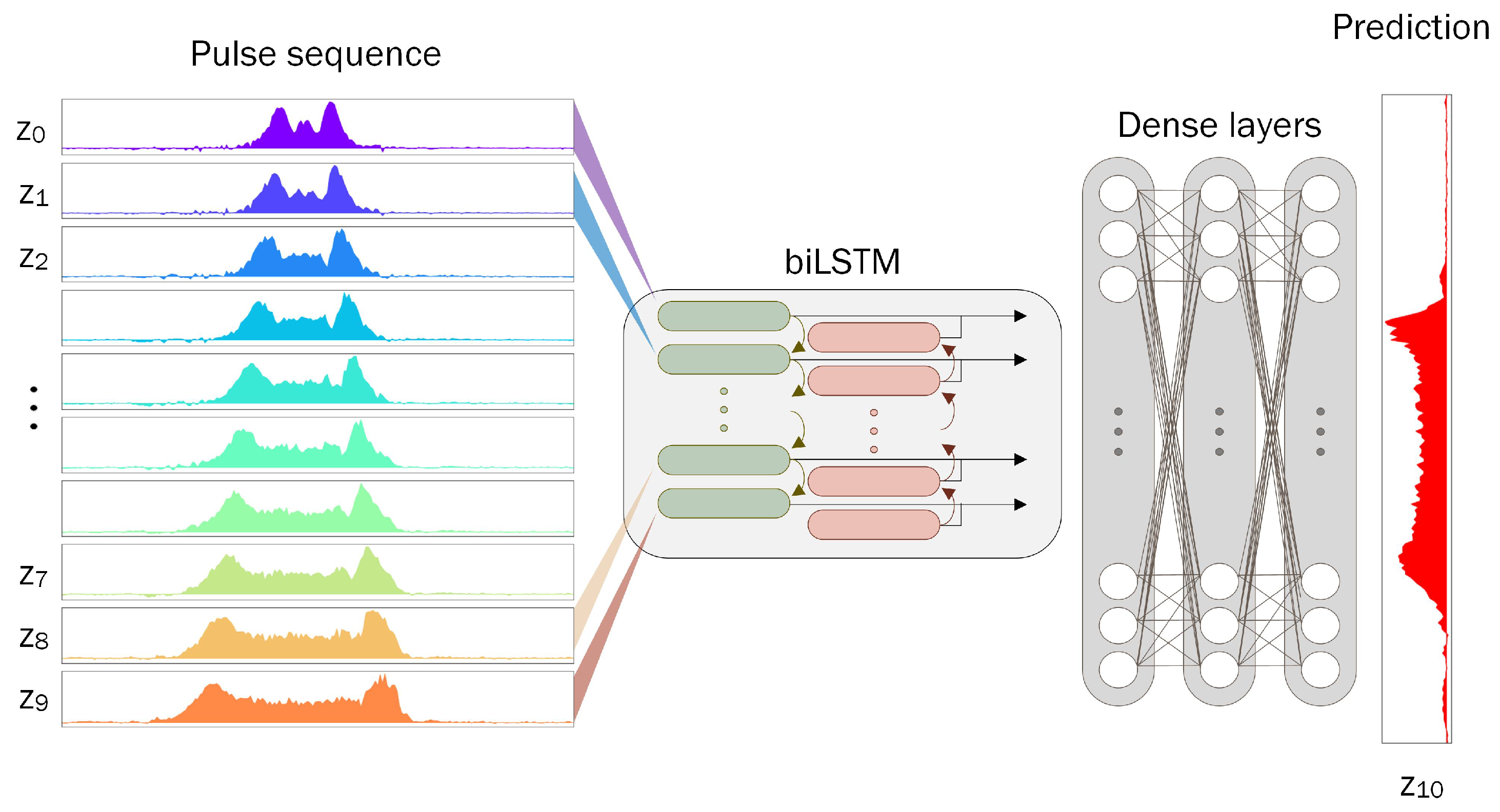
The recurrent neural network’s architecture is depicted in
Figure 1.
Here, we employ two neural networks with similar structures to predict spectral and temporal intensity evolution independently.
4. Data Preparation and Training Process
The RNN was trained with synthetic data generated using the model described in
Section 2. The chosen range of initial pulse parameters spans the variation in the relationship between dispersion and nonlinear length, ranging from 0.25 to 250. The initial pulse intensity is uniformly variable, ranging from 100 W to 1000 W, while the pulse width varies logarithmically from 0.1 to 10 ps. The explored parameter space encompasses a wide diversity of pulse propagation regimes, ranging from GGN amplification to pulse amplification, accompanied by the formation of noise Raman pulses in high-intensity cases [
19]. We selected a length of 7 m for the optical fiber, a choice deemed sufficient for stabilizing a nonlinear attractor, as suggested by Sidorenko et al. [
1]. The training dataset comprises 879 examples of pulse evolution within the specified range of initial parameters. The RNN is trained to forecast the evolution profile at fiber intervals of 46 mm, requiring 150 steps to predict the evolution along the entire length of the fiber. No preprocessing was applied to the data, except for reducing the resolution using linear interpolation along the temporal (spectral) coordinate, from 16384 to 500 points. The choice of this dimensionality reduction was based on the resolution needed to display fine spectral modulation dynamics and the computational resources available for training the neural network, and it can be varied for different problems.
The dataset utilized for testing the model consisted of displaced grid points within the same initial pulse parameter interval. To ensure the construction of a reliable model capable of accurately predicting the evolution of different propagation regimes on a uniform grid, it is essential to employ test and train datasets of equal size and distribution. Therefore, maintaining a 1:1 test-to-train ratio is imperative to effectively assess the prediction performance of the neural network within the chosen parameter range for this task.
The data for training and testing the neural network are prepared using the sliding window method illustrated in
Figure 2a. This technique facilitates the division of the data into smaller segments. The first ten intensity profiles are interpreted as the neural network input, with the subsequent one serving as its target output. The window then slides by one point over the fiber length and repeats the process until the end of the training evolution. After creating 10+1 pairs, it is essential to shuffle these pairs from all the training evaluations to ensure a stable learning process. The prepared data are then fed into the neural network during the training process.
To find the global minimum in the loss function and ensure effective training, we employed several optimization and learning stabilization techniques. These included the Adam optimizer, hyperparameter tuning, and a learning rate scheduler. By utilizing these techniques, we aimed to enhance the training efficiency and stability of our model. Model training was performed on a local server using an NVIDIA RTX 4090 graphics processing unit (GPU).
5. Results
We used an autoregression approach to reconstruct the prediction. This method allows the neural network to forecast the data evolution for any number of steps forward by sequentially feeding its output back into its input.
5.1. Metrics Used for Tracking RNN Performance
Here, we outline the metrics used to assess the final predictive performance of the trained neural network. The network is trained to predict a single pulse profile by leveraging the evolution dynamics extracted from a sequence of profiles using the mean squared error (MSE) loss:
where
I represents the temporal (spectral) intensity array at a fixed z coordinate along the fiber, and
N denotes the size of the temporal (spectral) domain.
In autoregression prediction, the model effectively handles newly self-generated data that were not part of the training sample. To evaluate the final result, a different metric was employed. The normalized root mean square error (NRMSE) metric, widely utilized in similar tasks, provides a robust accuracy estimation for predicting errors in individual intensity profiles.
However, when applied to the entire evolution map, the NRMSE tends to overestimate errors in the case of low-energy pulses with narrow spectra and underestimate errors in high-energy propagation regimes. Additionally, interpreting the quality of the prediction is not straightforward. In an attempt to address these issues, we propose using another version of the normalized MSE—the peak signal-to-noise ratio (PSNR) metric [
20]:
where
is a 2D array that represents the evolution of a temporal (spectral) intensity array along the spatial coordinate
z.
The PSNR is frequently employed for assessing the quality of reconstructed images and offers several advantages over the NRMSE metrics, including a decibel scale and normalization based on the maximum intensity.
5.2. Forecasting of Temporal and Spectral Intensity Evolution
We assessed the prediction error of the PI-RNN model using Equation (
7) and depicted the temporal and spectral intensity maps in
Figure 3a and
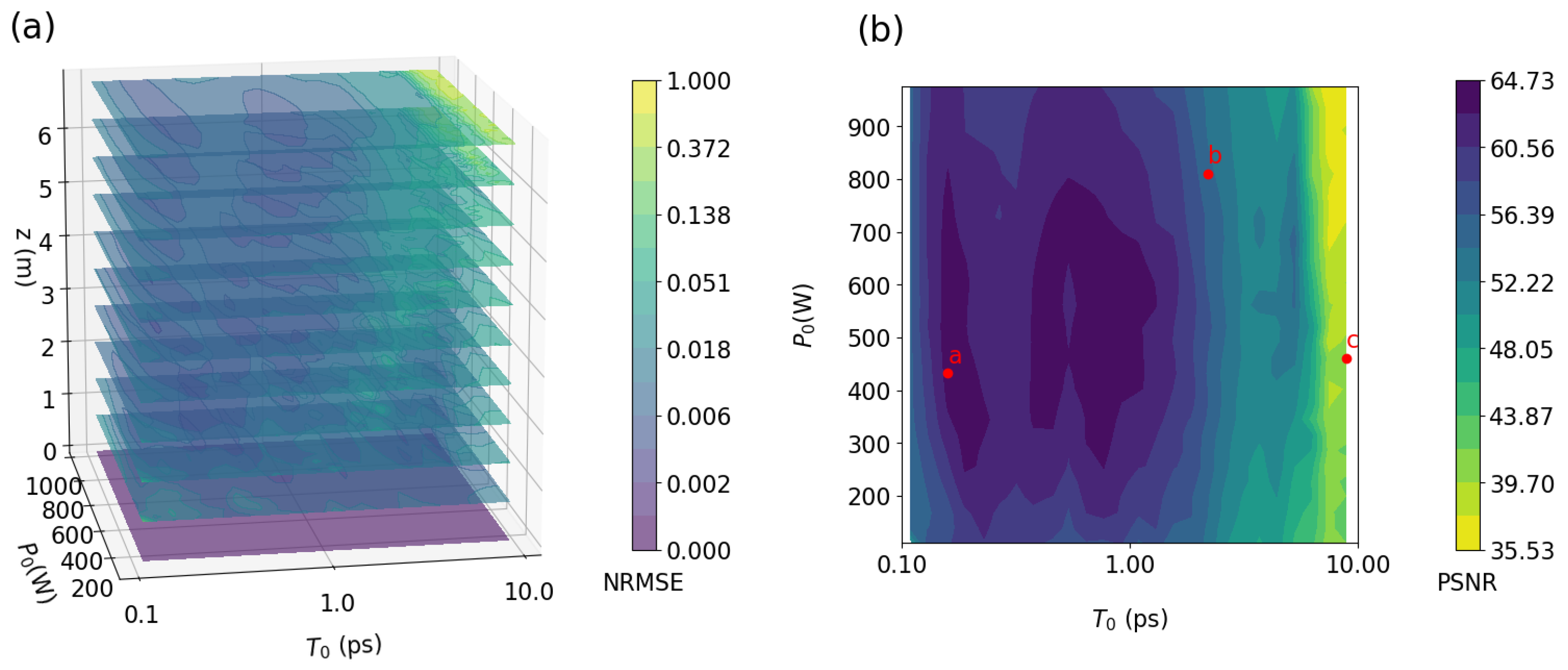
Figure 4a, respectively. The plots illustrate the smooth evolution of errors along the fiber for all initial pulse parameters, with no discernible discontinuities or outliers within the prediction maps.
Figure 3b and
Figure 4b, calculated using Equation (
8), illustrate the comprehensive error maps across the plane of initial pulse parameters. These maps reveal the impact of initial pulse parameters on the overall PSNR error along the fiber. The interpretation of the error diagrams is as follows: the prevailing trend indicating the most significant errors corresponds to situations with numerous high-intensity modulation peaks or noise-like generation. Specifically, in the prediction of the temporal evolution, the highest accumulated error is associated with the Raman generation. When predicting the spectral evolution, the highest error is associated with regions exhibiting significant nonlinear phase accumulation before transitioning to a smooth attractor-like regime or regions characterized by the emergence of a noisy Raman pulse.
We conducted tests on various data preprocessing methods, including normalization and logarithmic transformation, which have demonstrated effectiveness for passive fibers, as reported in previous works [
8,
9]. However, we observed that these methods diminished the information content of the spectral intensity evolution within the active fiber. Recognizing the significance of spectral intensity amplitude as an additional feature aiding the neural network in precise predictions and evolution stage determination through autoregression, we opted to use the spectral intensity data in the original linear scale without any preprocessing.
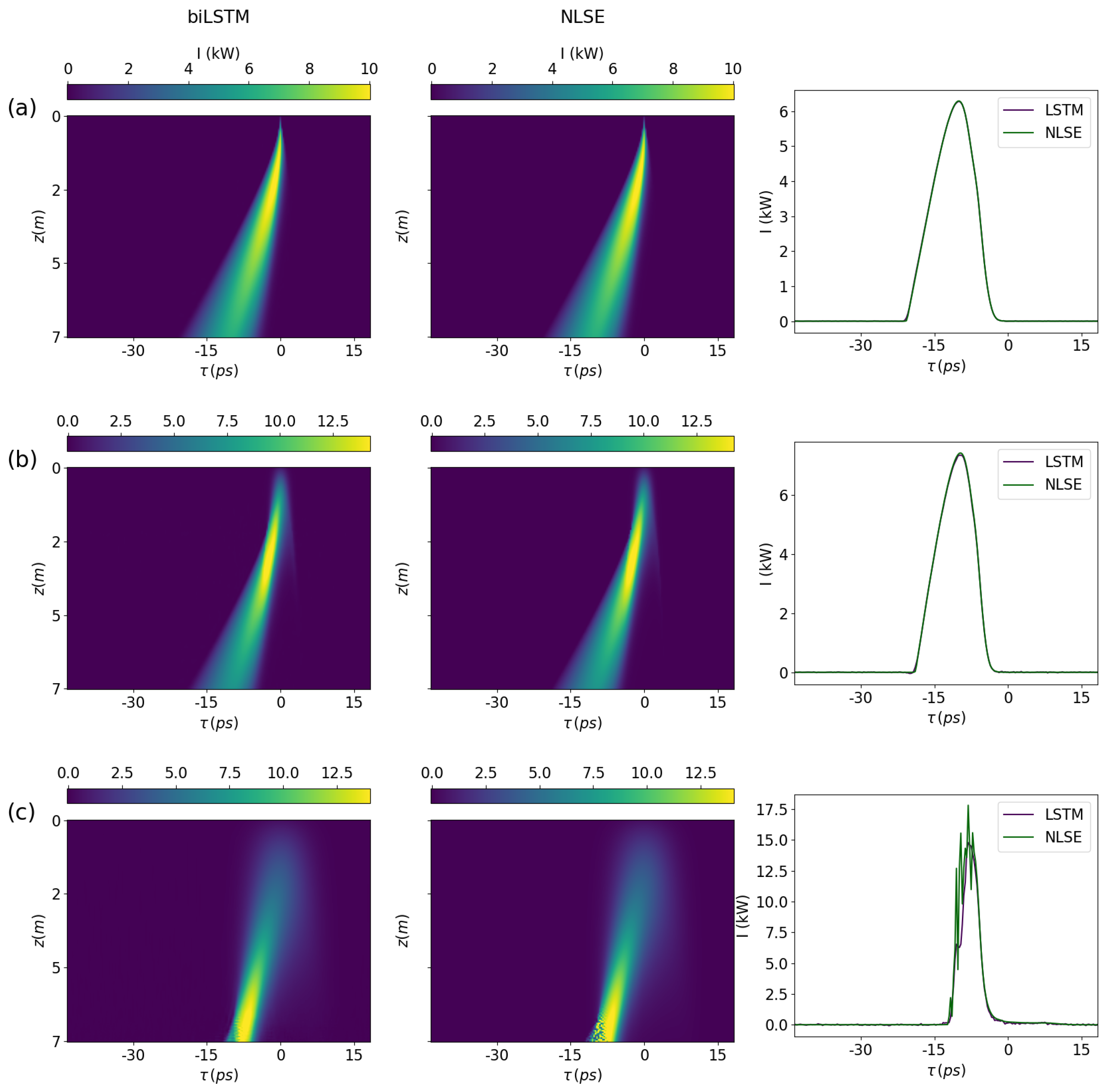
To compare pulse propagation maps predicted by the PI-RNN with numerical modeling using the NLSE, we picked three distinctive regimes from the data. Three main types of behaviors include a smooth GGN regime resulting in a formation of a nonlinear attractor, a transient regime, and a regime showing a pronounced influence of the stimulated Raman scattering on a pulse amplification.
Figure 5 shows examples of the temporal evolutions, along with their locations in the error map displayed with red labeled points in
Figure 3b.
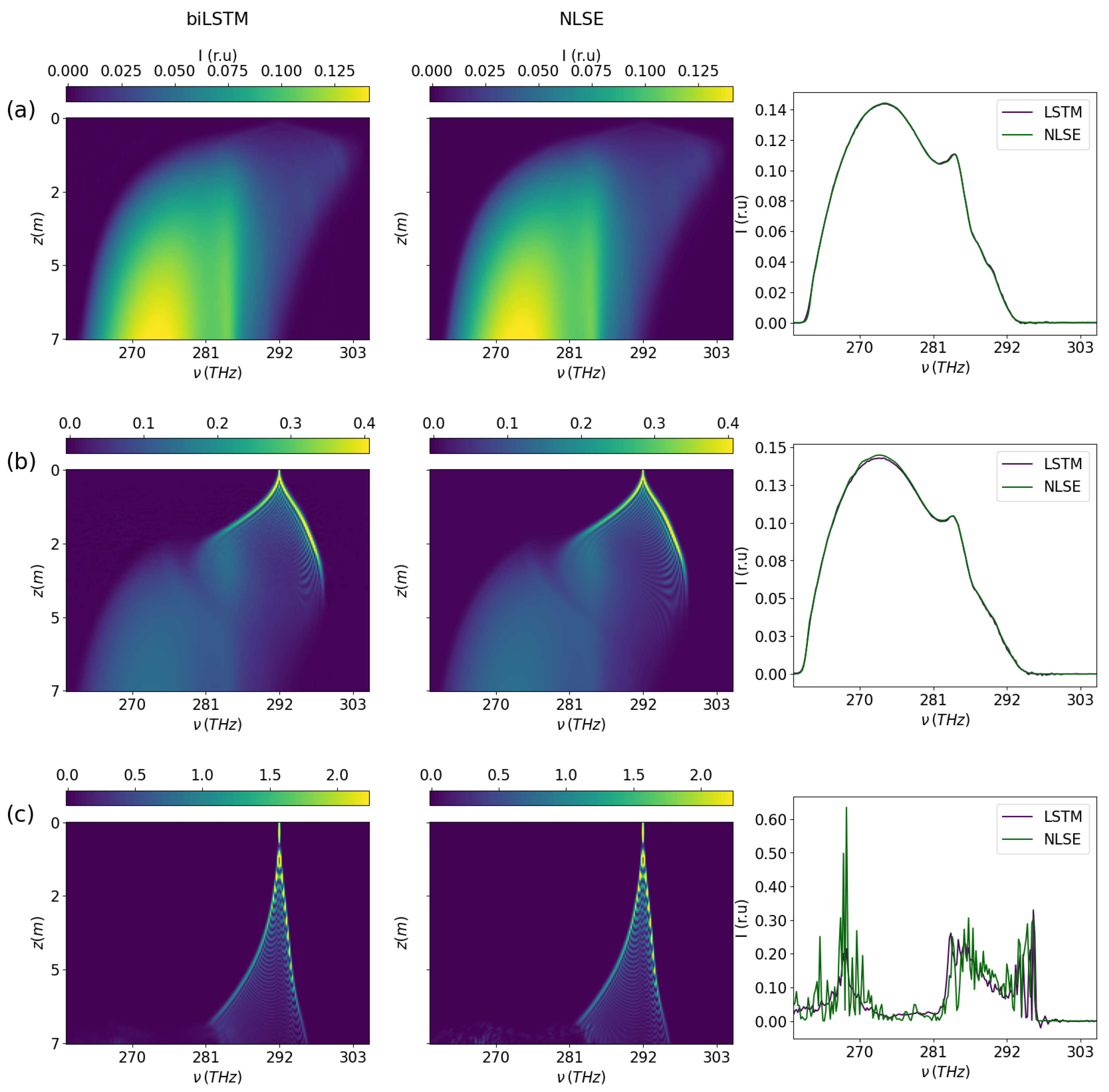
Figure 6 shows typical spectral intensity propagation regimes, with their locations in the error map in
Figure 4b. The Raman scattering manifests itself as the generation of a noise-like pulse with energy comparable to the main pulse, downshifted by about 13.2 THz in frequency (
Figure 6c) [
21].
The PI-RNN demonstrates its capability to model the temporal and spectral evolution for any point within the training parameter area.
Autoregressive reconstruction of the evolution map along the 7-meter-long fibre, as presented in the
Figure 5 and
Figure 6, takes about 0.05 s with PI-RNN. This is approximately 700 times faster than the fastest paralleled numerical NLSE model when using the NVIDIA RTX 4090 GPU and 2000 times faster than the conventional CPU-based numerical model. This notable difference is attributed to the reduction in the number of numerical operations required for each step along the fiber, a decrease in the total number of steps needed to obtain a solution, and the lower temporal (spectral) resolution required for the computations. The final PI-RNN model has an estimated tens of millions of trainable parameters.
5.3. Resistance to Noise
The neural network, trained on undisturbed synthetic data, was found to be robust to external noise in the test dataset. The PI-RNN can capture the pulse propagation regime up to the signal-to-noise ratio values of 20 dB. Specifically, when given an initial pulse with added ’white’ Gaussian noise, the neural network predicts the output pulse with noise suppression. This feature allows for greater practical significance of this study in the future, as it can handle realistic experimental data that may contain noise or other imperfections.
5.4. Autoregression Problems
Overfitting poses a significant challenge in autoregressive prediction problems. In autoregressive predictions, the neural network establishes a feedback loop, using slightly perturbed input data influenced by its own prediction errors to make subsequent predictions. This feedback loop complicates the monitoring and prevention of overfitting, since the neural network is only trained to predict only one step initially and is not explicitly trained for autoregressive prediction. Even though the model has high accuracy for one-step prediction on a validation dataset, it may face issues when estimating autoregressive predictions on a test dataset. The slightly undertrained model seems to be more robust to overfitting the numerical modeling data when predicting the evolution autoregressively.
5.5. Cold Start Problems
Cold start is a method of evolution reconstruction that starts with a single initial pulse profile, which is then fed to all RNN inputs. This method facilitates the reconstruction of the autoregressive evolution map using only a single pulse profile, thereby simplifying its application for various tasks.
To improve the model’s performance in cold start prediction scenarios, we used a specific approach to prepare the training data. The main concept involves incorporating “cold start data” into the training sample, as shown in
Figure 2b. “Cold start data” are a synthetic type of data that mimic the model’s task of reconstructing evolution from one tiled initial profile. The basic idea is to replace the first
n evolution profiles, where
n is the number of inputs for the recurrent neural network, with the initial profile. This approach aids the model in improving predictions by learning from these artificial examples.
We obtained results with comparable accuracy for predicting cold start temporal and spectral evolutions as the prediction based on the starting pulse sequence.
6. Conclusions
In this paper, we explored the potential of using PI-RNN to predict the evolution of spectral and temporal pulse intensity along the fiber amplifier—a computationally challenging task in nonlinear optics. We introduced an updated PI-RNN architecture designed to learn the complex dynamics of the optical field from a large dataset generated via numerical simulations and conducted a thorough evaluation of its performance. We found that the PI-RNN can accurately and precisely estimate the evolution map, outperforming the conventional split-step numerical solution of the NLSE by a significant margin—2000 times faster. This improved speed persists even when parallelized with a GPU, resulting in a 660-fold faster computation.
Furthermore, the PI-RNN adeptly performs interpolation and extrapolation of the field evolution along the fiber with reasonable accuracy. It exhibits adaptability to various grid sizes along the z-coordinate. Notably, a single neural network proved capable of capturing diverse propagation regimes, making it a universal tool for investigating dynamics within the chosen parameter space. The PI-RNN approach can achieve further enhancement by integrating experimental data into the training set. This can not only improve the time performance but also enhances its descriptive capabilities, surpassing numerical modeling.
We have also detailed the challenges encountered during the PI-RNN training process for autoregressive prediction tasks. One significant drawback identified in reconstructing the entire evolution map using PI-RNN is its cold start prediction performance, heavily dependent on the data sample provided. To address this issue, we introduce a novel approach to preparing training data, resulting in improved cold start execution. This modification leads to notable performance enhancements, particularly in predicting the temporal intensity map using a single input profile.
In conclusion, we assert that the PI-RNN has proven to be a promising technique for predicting the evolution of pulse intensity along an active fiber, demonstrating substantial advantages over traditional numerical methods.
Author Contributions
Conceptualization, A.B.; methodology, K.S. and A.B.; software, K.S.; validation, A.B. and K.S.; investigation, K.S. and A.B.; writing—original draft preparation, K.S. and A.B., visualization, K.S. All authors have read and agreed to the published version of the manuscript.
Funding
This research was funded by the Ministry of Science and Higher Education of the Russian Federation (Project No. FSUS-2021-0015).
Institutional Review Board Statement
Not applicable.
Informed Consent Statement
Not applicable.
Data Availability Statement
The data presented in this study are available on request from the corresponding author.
Conflicts of Interest
The authors declare no conflicts of interest.
Abbreviations
The following abbreviations are used in this manuscript:
| PI-RNN | Physics-informed recurrent neural network. |
| NLSE | Nonlinear Schrodinger equation. |
| LSTM | Long short-term memory. |
| MSE | Mean square error. |
| PSNR | Peak signal-to-noise ratio. |
| GPU | Graphics processing unit. |
References
- Sidorenko, P.; Fu, W.; Wise, F. Nonlinear ultrafast fiber amplifiers beyond the gain-narrowing limit. Optica 2019, 6, 1328–1333. [Google Scholar] [CrossRef] [PubMed]
- Chen, Y.H.; Sidorenko, P.; Thorne, R.; Wise, F. Starting dynamics of a linear-cavity femtosecond Mamyshev oscillator. JOSA B 2021, 38, 743–748. [Google Scholar] [CrossRef] [PubMed]
- Turitsyn, S.K.; Bednyakova, A.E.; Podivilov, E.V. Nonlinear Optical Pulses in Media with Asymmetric Gain. Phys. Rev. Lett. 2023, 131, 153802. [Google Scholar] [CrossRef] [PubMed]
- Boscolo, S.; Dudley, J.M.; Finot, C. Modelling self-similar parabolic pulses in optical fibres with a neural network. Results Opt. 2021, 3, 100066. [Google Scholar] [CrossRef]
- Stanfield, M.; Ott, J.; Gardner, C.; Beier, N.F.; Farinella, D.M.; Mancuso, C.A.; Baldi, P.; Dollar, F. Real-time reconstruction of high energy, ultrafast laser pulses using deep learning. Sci. Rep. 2022, 12, 5299. [Google Scholar] [CrossRef] [PubMed]
- Freire, P.; Manuylovich, E.; Prilepsky, J.E.; Turitsyn, S.K. Artificial neural networks for photonic applications—From algorithms to implementation: Tutorial. Adv. Opt. Photon. 2023, 15, 739–834. [Google Scholar] [CrossRef]
- Boscolo, S.; Finot, C. Artificial neural networks for nonlinear pulse shaping in optical fibers. Opt. Laser Technol. 2020, 131, 106439. [Google Scholar] [CrossRef]
- Salmela, L.; Tsipinakis, N.; Foi, A.; Billet, C.; Dudley, J.M.; Genty, G. Predicting ultrafast nonlinear dynamics in fibre optics with a recurrent neural network. Nat. Mach. Intell. 2021, 3, 344–354. [Google Scholar] [CrossRef]
- Teğin, U.; Dinç, N.U.; Moser, C.; Psaltis, D. Reusability report: Predicting spatiotemporal nonlinear dynamics in multimode fibre optics with a recurrent neural network. Nat. Mach. Intell. 2021, 3, 387–391. [Google Scholar] [CrossRef]
- Kirsch, D.C.; Bednyakova, A.; Varak, P.; Honzatko, P.; Cadier, B.; Robin, T.; Fotiadi, A.; Peterka, P.; Chernysheva, M. Gain-controlled broadband tuneability in self-mode-locked Thulium-doped fibre laser. Commun. Phys. 2022, 5, 219. [Google Scholar] [CrossRef]
- Turitsyn, S.K.; Bednyakova, A.E.; Fedoruk, M.P.; Latkin, A.I.; Fotiadi, A.A.; Kurkov, A.S.; Sholokhov, E. Modeling of CW Yb-doped fiber lasers with highly nonlinear cavity dynamics. Opt. Express 2011, 19, 8394–8405. [Google Scholar] [CrossRef] [PubMed]
- Dong, L. Nonlinear Propagation in Optical Fibers With Gain Saturation and Gain Dispersion. J. Light. Technol. 2020, 38, 6897–6904. [Google Scholar] [CrossRef]
- Chen, H.W.; Lim, J.; Huang, S.W.; Schimpf, D.N.; Kärtner, F.X.; Chang, G. Optimization of femtosecond Yb-doped fiber amplifiers for high-quality pulse compression. Opt. Express 2012, 20, 28672–28682. [Google Scholar] [CrossRef] [PubMed]
- Agrawal, G.P. Nonlinear Fiber Optics, 4th ed.; Elsevier: Amsterdam, The Netherlands, 2006. [Google Scholar]
- Hollenbeck, D.; Cantrell, C. Multiple-vibrational-mode model for fiber-optic Raman gain spectrum and response function. J. Opt. Soc. Am. B 2002, 19, 2886. [Google Scholar] [CrossRef]
- Bolt, D. Pyofss. 2013. Available online: https://github.com/LeiDai/pyofss (accessed on 15 December 2023).
- Efremov, V.D.; Evmenova, E.A.; Antropov, A.A.; Kharenko, D.S. Numerical investigation of the energy limit in a picosecond fiber opticparametric oscillator. Appl. Opt. 2022, 61, 1806–1810. [Google Scholar] [CrossRef] [PubMed]
- Paszke, A.; Gross, S.; Chintala, S.; Chanan, G.; Yang, E.; DeVito, Z.; Lin, Z.; Desmaison, A.; Antiga, L.; Lerer, A. Automatic differentiation in pytorch. In Proceedings of the 31st Conference on Neural Information Processing Systems (NIPS 2017), Long Beach, CA, USA, 4–9 December 2017. [Google Scholar]
- Bednyakova, A.E.; Babin, S.A.; Kharenko, D.S.; Podivilov, E.V.; Fedoruk, M.P.; Kalashnikov, V.L.; Apolonski, A. Evolution of dissipative solitons in a fiber laser oscillator in the presence of strong Raman scattering. Opt. Express 2013, 21, 20556–20564. [Google Scholar] [CrossRef] [PubMed]
- Samajdar, T.; Quraishi, M.I. Analysis and evaluation of image quality metrics. In Information Systems Design and Intelligent Applications: Proceedings of Second International Conference INDIA 2015, Kalyani, India, 8–9 January 2015; Springer: Berlin/Heidelberg, Germany, 2015; Volume 2, pp. 369–378. [Google Scholar]
- Agrawal, G.P. Nonlinear fiber optics. In Nonlinear Science at the Dawn of the 21st Century; Springer: Berlin/Heidelberg, Germany, 2000; pp. 195–211. [Google Scholar]
| Disclaimer/Publisher’s Note: The statements, opinions and data contained in all publications are solely those of the individual author(s) and contributor(s) and not of MDPI and/or the editor(s). MDPI and/or the editor(s) disclaim responsibility for any injury to people or property resulting from any ideas, methods, instructions or products referred to in the content. |
© 2024 by the authors. Licensee MDPI, Basel, Switzerland. This article is an open access article distributed under the terms and conditions of the Creative Commons Attribution (CC BY) license (https://creativecommons.org/licenses/by/4.0/).

