Adaptive Threshold Algorithm for Outlier Elimination in 3D Topography Data of Metal Additive Manufactured Surfaces Obtained from Focus Variation Microscopy

Abstract

The topography of surfaces produced by metal additive manufacturing is a challenge for optical measurement systems such as focus variation microscopes. These irregularities can lead to artifacts, such as incorrectly measured protrusions or spikes, hampering reliable topographic characterization. In order to eliminate this problem, we introduce a new algorithm based on dual convolving a vertical Sobel operator with cross sections of an image stack parallel to the scanning direction of the so-called depth scan. This has proven beneficial in order to distinguish the focus region from out-of-focus areas where outliers are frequently detected. This paper introduces a method for deriving self-adaptive thresholds from the convolution result and compares the effects of different operators in creating self-adaptive thresholds. Additionally, a simulation model of focus variation microscopy is introduced to validate both the measuring system and the proposed algorithm, thereby enhancing the overall performance of focus variation microscopy. Finally, comparisons of measurement results on rough metal additive manufacturing workpieces with and without self-adaptive thresholds are discussed to demonstrate the algorithm’s effectiveness.The utilization of self-adaptive thresholds demonstrably reduces the uncertainty range in roughness parameter calculations. For example, in the case of an additive manufactured metal sample due to outlier elimination, the $Sz$ roughness value reduces from 543 µm to 413 µm.

1. Introduction

In recent decades, the development of optical 3D-microscopy has significantly advanced the characterization and reconstruction of surface topography, which is increasingly important in various industrial fields. Characterizing surface topography essentially involves managing the manufacturing process, thereby enabling the modification and improvement of the functionality of targeted workpieces [1,2] here reference is added. Measuring certain critical surfaces, such as those produced by metal additive manufacturing (MAM), is particularly challenging due to their strong surface irregularities, which include sharp and rounded protrusions, deep undercuts, and grooves. Consequently, reflectivity varies across different regions, leading to overexposure of camera images in some areas while others remain dark [3,4]. The steep slopes of surface microtexture can exceed the measurement limitations of certain optical systems [5,6], resulting in artifacts like spikes or unexpected protrusions on the reconstructed surface topography. These artifacts affect the accuracy of calculating roughness parameters due to rapid changes in surface heights and can misrepresent surface texture. Therefore, detecting and removing these artifacts is essential to obtain accurate topography data for reliable surface analysis [1].

The topography of MAM surfaces can generally be measured using tactile stylus instruments, X-ray computer tomography (XCT), or optical instruments [7]. These optical instruments include coherence scanning interferometers (CSI) [8], confocal microscopes (CM) [9], and focus variation microscopy (FVM) [10], among others. FVM offers several advantages for reconstructing MAM surfaces, including the application of ring light illumination with multilayer LEDs to complement coaxial illumination, providing a more comprehensive observing view. Additionally, this combination mitigates the effects of numerical aperture (NA) limitations, unlike CSI or CM. For more details related to the construction of FVM relevant to this work, we refer to [11,12]. Additionally, the relevant optical components are presented in

Table 1. Optical component parameters utilized in the experimental setup [13].

Optical Components	Specification
Coaxial illumination	Single high-power green LED (λ = 520 nm, Pmax = 126 mW);
Ring light	Custom-built dome-shaped;
	approx. 100 red LEDs (λ = 623 nm) arranged in three rings;
Working distance	approx. 19 mm;
Objective lens	Magnification: 10; Numerical aperture (NA): 0.45;
Camera	ALLIED VISION GF146B ASG Guppy CCD camera (Allied Vision, Stadtroda, Germany); IEEE 1394a interface;
	1280 × 960 pixels with a field of view (FOV) of approx. 583 µm × 438 µm;
Depth of field	5.2 µm (for 520 nm, calculated using $2\times {\displaystyle \frac{\lambda }{{\mathrm{NA}}^2}}$);
Lateral resolution	0.58 µm (for 520 nm, calculated using ${\displaystyle \frac{\lambda }{2\times \mathrm{NA}}}$);

.

To achieve height discrimination, the FVM system performs a so-called depth scan. During this process, the distance between the object under investigation and the FVM is continuously varied, capturing images of the workpiece surface at equidistant steps. This results in a series of images known as an image stack. In this study, the horizontal plane of the images is aligned with the $xy$-plane, making the z-direction the scanning direction. The vertical range of the depth scan performed by the FVM is adjusted so that the most relevant information about the surface under investigation is located vertically in the center of the image stack. The data near the central vertical region of the image stack exhibit a common feature, namely that some areas are in focus while others are defocused. Consequently, a small square of neighboring pixels in the $xy$-plane relative to each pixel within the image stack changes from defocus to focus and back to defocus along the z-axis. All focus positions related to all pixels on a camera contribute to the reconstruction of the surface topography to be measured.

To address artifacts in reconstructed topography, previous research has focused on spike-removal filters [14], such as morphological filters that use a rolling ball to identify spike positions [15]. However, this method can be time-consuming, especially when dealing with reconstructed textures containing numerous spikes. More common spike-detection methods involve thresholds related to the maximum and minimum valid height values, thus excluding out-of-focus heights. Previous studies often use a constant threshold for all determined height values to detect spikes. This threshold can be determined simply by a fraction of the maximum height value if spikes are well-separated from surface positions [1] or by analyzing the height distribution [16]. The threshold is typically directly applied to the height values after topography reconstruction [17]. Moreover, thresholds can be dynamically adjusted to different surface areas of interest to adapt to rapid height changes [11,12]. Another approach is to apply a threshold to height values after separating the original surface into a low-pass filtered component and a residual surface, with the threshold applied only to the residual surface [18]. Additionally, thresholds can be applied to other physical quantities such as power spectral density (PSD) to detect spikes by treating them as high-frequency errors [19] or to detail coefficients associated with decomposed surface information, where the threshold is used to select the spikes [20].

Among the mentioned methods, employing pairs of self-adaptive thresholds positioned above and below the reconstructed topography may be especially effective for eliminating spikes in MAM textures. However, these thresholds can also be applied before the reconstruction of the topography, as demonstrated in the study of Xu et al. [11]. They introduced such a method, translating the reconstruction of a pair of three-dimensional self-adaptive threshold topographies (for both upper and lower limits for valid height values) into a series of pairs of two-dimensional self-adaptive threshold profiles (SATP) located in $xz$- or $yz$- planes to restrict the range of the z-axis used for focus searching. Typically, the entire vertical range of the depth scan, i.e., the z-axis, is utilized. They employ the vertical Sobel operator twice, aiding the construction of the SATP by enhancing the contrast between the region of focus (ROF) and the region of defocus (RODF). This paper aims to introduce an algorithm to construct such an SATP and compare the effects of different operators on their construction.

The proposed algorithm relies on images captured using a self-constructed FVM [11,12]. A significant advantage of employing this system is the need for raw and unprocessed datasets to assess the effectiveness of introducing an SATP.

The contributions of this study are outlined as follows:

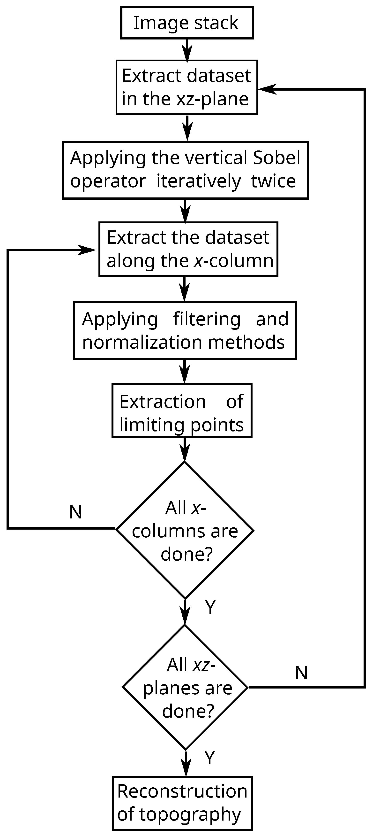
• Detailed explanation of the construction of a pair of SATP for each $xz$-plane to determine the ROF, where the focus position is highly probable;
• Comparison of several constructed SATPs based on different operators;
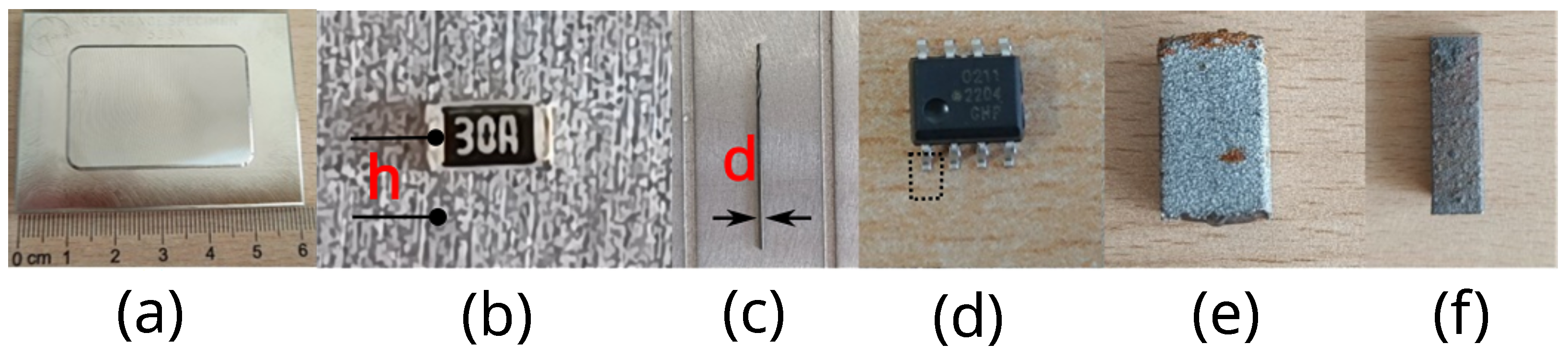
• Validation of the findings by measuring several electrical components with microscale dimensions due to the lack of a standard MAM workpiece, as per the authors’ knowledge;
• Validation of the findings involves measuring the texture of a Rubert precision reference standard 525C, which features quite smooth surfaces, and then adding additional roughness using a virtual FVM instrument.
• Prevention of most artifacts from appearing on the initially reconstructed surface texture, thereby eliminating the need for removing invalid pixels as generally utilized in previous studies.

2. Methodology

2.1. Samples for Simulation, Validation and Experiments

In this section, the measurement samples used for validation are introduced. Initially, a microtexture standard, Rubert 525C, which features a specular surface in reality with a sinusoidal texture of peak-to-valley (PV) amplitude 19 µm and a period length of 135 µm, as shown in Figure 1a, serves as the validation standard in the absence of an MAM standard. Given the impracticality of physically adding roughness to Rubert 525C (Rubert & Co Ltd., Cheadle, United Kingdom), a simulation model [21] is employed, which virtually adds additional roughness to the Rubert 525C sample. In previous works, measurements obtained by different instruments were used for validation. However, discrepancies in measured profiles of rough surfaces obtained by different instruments can reach up to 60%, as reported in [22]. Consequently, this type of validation is not considered here.

Further objects used for validation include an electrical resistor, a metal drill, and an optically-coupled logic gate, as illustrated in Figure 1b–d, respectively. The measured dimensions are as follows: the height ‘h’ (see Figure 1b) of the resistor (SMD-RCM x), defined as the vertical distance between the top of the resistor and an aluminum baseplate, is 0.45 mm ± 0.05 mm as specified by the manufacturer. The diameter of the drill’s shaft, measured between two black arrows (see Figure 1c), is 0.5 mm, with a caliper measurement uncertainty of 0.05 mm. The datasheet for the logic gate (HCPL-0211) produced by Avago Technologies (San Jose, CA, USA) indicates a leg width of 0.406 mm ± 0.076 mm, marked by a dashed black box (see Figure 1d). Additional measurements pertain to MAM workpieces, MAM1 in Figure 1e, and MAM2 in Figure 1f. These workpieces exhibit high roughness, enabling the comparison of the improved performance using the proposed SATP against the performance without them.

2.2. Proposed Algorithm to Construct the SATP

Figure 2 presents a flowchart illustrating the complete procedure, implemented in Python, developed for the construction of the SATP. As mentioned earlier, the idea of the SATP is to select ROF, covering the entire x-axis, in each $xz$-plane of an image stack [11]. A dataset of an $xz$-plane corresponding to MAM2 is shown in Figure 3a, with part of the ROF from $x\approx 300$ µm to $x\approx 450$ µm highlighted by the dashed green box. The two areas above and below this highlighted region are part of the RODF. Within the ROF, intensities alternate more frequently compared to the RODF, allowing the algorithm to set SATPs that separate the ROF from the RODF.

Figure 3b presents the reconstructed profile, depicted by the red curve, alongside the dataset shown in Figure 3a, emphasizing the importance of constructing SATPs. In the absence of SATPs, the areas labeled as no. 1, 2, 3, and 4 in Figure 3b exhibit significant artifacts, while No. 5 displays a type of artifact that can be overlooked easily. This artifact no. 5, appearing as a small spike pointed out by a red arrow in Figure 3b, is characterized as a defocus issue, as explained by Xu et al. [12], where defocus issues produce significant artifacts that cannot be overlooked. It arises from gray level gradients observed within the dashed red box, highlighted on its left side in Figure 3a. These gradients, formed between relatively brighter and darker regions, sometimes exhibit higher contrast compared to the corresponding focal position. If they are not excluded, such contrast values are used for focus detection in the evaluation of the FVM image stack. As a result, these regions with gray level gradients should be excluded from the ROF.

The remaining artifacts can be categorized into two types: unexpected protrusions (no. 1, 2, and 3) and spikes (no. 4). These artifacts are found in sections such as undercuts, grooves, and steep slopes, where only a small amount of light is captured by the camera. This issue is common when reconstructing MAM topographies, as protrusion artifacts also appear in results obtained by commercial systems, as described in [23]. Although it is easy to find a constant threshold for selecting artifacts on this specific $xz$-plane, the irregularity of the MAM surface makes it inappropriate to apply the same constant threshold to other $xz$-planes without affecting non-artifact areas. This challenge is addressed through the use of SATPs, which will be demonstrated in detail in Section 3.3.

SATP appear as pairs at each x-axis position for each $xz$-plane, one above and one below the ROF. Constructing such a pair starts with the analysis of an z-column, illustrated as a dashed white line in Figure 3b for $x\approx$ 205 µm, defined as the dataset obtained by one pixel along the z-axis. The dataset of this z-column is shown in Figure 3c. The region between z values of 500 µm and 750 µm, represented by points L1 and L2, belongs to the ROF according to Figure 3b. Intensities within this region change rapidly, while those outside change relatively slowly. Therefore, L1 and L2 are the rough boundaries separating the ROF and the RODF, defined here as a pair of limiting points (LP). The approximate positions of LPs vary when using different processing algorithms (e.g., different operators).

The intensity signals for each pixel corresponding to each x-column in Figure 3b provide a pair of LPs. These LPs play a key role in constructing a pair of SATPs for each $xz$-plane. Essentially, constructing a pair of SATPs entails forming a sequence of LP pairs. The direct LP identification using Figure 3c is possible but complex. For instance, the most dominant frequency components within the ROF after low-pass filtering should exceed the corresponding components within the RODF. However, the determination of LPs becomes much easier if a suitable operator, such as the vertical Sobel operator, is used to filter the intensity values in Figure 3a.

The mathematical expressions of the operators involved are displayed in the following equations:

$$S_{\mathrm{v}}=\left[\begin{array}{ccc}-1& 0& 1\\ -2& 0& 2\\ -1& 0& 1\end{array}\right]$$

(1)

$$S_{\mathrm{h}}=\left[\begin{array}{ccc}-1& -2& -1\\ 0& 0& 0\\ 1& 2& 1\end{array}\right]$$

(2)

and

$$L=\left[\begin{array}{ccc}0& 1& 0\\ 1& -4& 1\\ 0& 1& 0\end{array}\right]$$

(3)

The results obtained after convolving the dataset in Figure 3a with the vertical Sobel operator ($S_{\mathrm{v}}$), the horizontal Sobel operator ($S_{\mathrm{h}}$), and the Laplacian operator (L) individually are depicted in Figure 3d–f, respectively. The minimum and maximum values of the colorbar for each figure have been adjusted to enhance the visibility of ROFs. These operators increase the contrast between the ROF and the RODF, simplifying LP determination. This improvement is due to the widespread application of these operators in boundary detection, where the ROF is characterized by numerous rapidly changing intensities, forming densely packed quasi-boundaries, while the RODF generally lacks such features except for gradients.

When comparing the maximum values in these colorbars, it is evident that the contrast in Figure 3d is the most prominent among the three operators. Additionally, the gradients within the area marked by a dashed red box in Figure 3e are more pronounced compared to the same area in Figure 3a, resulting in more defocus issues. Therefore, the vertical Sobel operator has been demonstrated to be superior compared to the other two operators.

To further enhance the contrast between the ROF and RODF, the vertical Sobel operator is used twice, and the result is depicted in Figure 3g. The regions indicated by green boxes in Figure 3d–g can be utilized to compare the contrasts for different operators. If we extract the same z-column ($x\approx$ 205 µm) in Figure 3g, the absolute values of the corresponding dataset are displayed in Figure 3h, where the ROF in the middle is much easier to identify compared to Figure 3c by using a constant threshold, for instance. However, a more effective approach before applying this constant threshold is to further utilize a moving average filter with a window size of 50 samples, for example, to reduce the noise. The result is illustrated in Figure 3i. Based on this curve, the full width at half maximum (FWHM) is calculated to obtain two boundaries marked by dashed blue and orange lines on both the left and right sides. The two cross points between the dashed lines and the z-axis provide us with two LPs, L1 and L2, with respect to the z-column. It is worth noting that L1 and L2 can be adjusted with a reasonable distance from each other to expand the ROF when necessary. This process is repeated for each z-column covering the entire x-axis. A sequence of pairs of LPs is obtained, forming a pair of SATPs represented by the blue and orange curves shown in Figure 4b. Figure 3j displays the evaluated profile (red curve) extracted using SATPs together with the dataset shown in Figure 3g, where artifacts do not appear anymore.

Note that LPs (indicated by blue and orange dots) may not be found for certain z-columns, resulting in the absence of valid LPs, as depicted in Figure 4a. This is partly attributed to the low signal-to-noise ratio (SNR) in the captured intensity signals, which does not always exhibit a high SNR as depicted in the curve shown in Figure 3h. The main incomplete areas are labeled as P1 to P5 in Figure 4a. P1 is situated in an area resembling a hole, while the others are located on steep slope areas. These gaps can be filled through linear interpolation, as illustrated in Figure 4b, to maintain geometric continuity. Furthermore, in Figure 4c,d, LPs determined by applying the vertical Sobel operator once and the Laplacian operator are depicted for comparison. Both operators exhibit a higher number of gaps, with the Laplacian operator showing only a few pairs of LPs, marked as P6 to P9. Note that all backgrounds in these figures correspond to the one shown in Figure 3a.

Using the vertical Sobel operator twice is akin to employing the second derivative, which enhances the contrast around sharply tapered regions more effectively than using the first derivative [24] citation is changed, equivalent to applying the Sobel vertical operator once. The reason why the Laplacian operator does not outperform the twice-applied vertical Sobel operator could be attributed to its incorporation of second derivative operations in both horizontal and vertical directions. This vertical derivation does not significantly enhance the contrast between the ROF and RODF, as observed in Figure 3c. Considering the vertical derivation alongside the horizontal derivation actually, diminishes the effect primarily achieved by the horizontal derivation, which accounts for the negative impact of using the Laplacian operator.

To determine focal positions within the ROF, standard deviations $\sigma$ at specific positions $(x,y,z)$, ranging between each pair of SATPs, are computed to represent the contrast values associated with those positions. A window covering a length of $(2n+1)$ pixels centered around each position $(x,y,z)$ is defined to calculate $\sigma$. The central pixel lies within the ROF, indicated by a black point in the extract of Figure 4b. In essence, the length of each contrast curve, formed by a series of $\sigma$ values along the z-axis, is limited by the SATPs rather than covering all z values. Mathematically, the standard deviation is expressed as:

$$\sigma (k,l,m)=\sqrt{{\displaystyle \frac{1}{{(2n+1)}^2-1}}\sum _{i=k-n}^{k+n}\sum _{j=l-n}^{l+n}{(I(i\Delta x,j\Delta y,m\Delta z)-\overline{I})}^2},$$

(4)

where ($k\Delta x,l\Delta y,m\Delta z$) are the coordinates of the central pixels inside the image stack. It is worth noting that $\Delta x$ and $\Delta y$ represent the intervals between two consecutive pixels in the x and y dimensions, respectively. $I(i\Delta x,j\Delta y,m\Delta z)$ with $(i,j)\ne (k,l)$ denotes the intensity of neighboring pixels surrounding the central pixel, and $\overline{I}$ represents the average intensity inside the window [25]. Throughout this study, the window size is set to 5 × 5 pixels, i.e., $n=2$.

2.3. Procedure to Characterize Surface Roughness

This section elucidates the subsequent processing of the reconstructed topography and the acquisition of roughness parameters using the topography analysis software ‘Mountains Map’ from Digital Surf. The surface roughness of a profile is commonly characterized by the arithmetic mean value $Ra$ and maximum peak-to-valley deviation $Rz$ [26] (here reference is added), while parameters $Sa$ and $Sz$ are employed for areal measurements. The latter parameters are utilized to characterize the roughness of the MAM surfaces discussed in Section 3.3.

For calculating roughness parameters, the field of view (FOV) of 0.59 mm × 0.44 mm, as determined by the self-constructed FVM system configuration, is insufficient for rough MAM surfaces, especially with higher $Ra$ values, such as 40 µm. Hence, stitching is necessary to enhance the informative value of the roughness parameters. According to DIN EN ISO 25178-601 [27], a profile length of at least 56 mm is required to determine meaningful roughness parameters for $Ra$ values between 10 µm and 50 µm. However, this exceeds the capability of the current FVM setup, which achieves a lateral scanning length (in one direction) of approximately 3 mm and covers eight reconstructed topographies. Moreover, the tilt angle of the topography is corrected after stitching, as this angle significantly affects the calculation of roughness parameters such as $Sa$ or $Sz$. Typically, tilt is caused by misalignment of the workpiece in the optical system. Subsequently, a median filter with a window size of 9 × 9 pixels is applied. Since the lateral sampling interval equals 4.65 µm, these filter dimensions can be justified. Finally, $Sa$ and $Sz$ values are calculated according to ISO 25178-2 [28] (described in ‘Mountains Map’), and the stitched topography is observed.

3. Results and Discussion

3.1. Validation by Simulation

The mathematical model used to simulate the transfer behavior of the current self-constructed FVM system is described by Pahl et al. [21]. Although the simulation model accounts for both coaxial illumination and ring light illumination, it simplifies the setup by considering a continuous light distribution for the ring light instead of the multilayer LEDs used in practice. Additionally, the mathematical model of Rubert 525C is represented as an ideal sinusoidal texture specified by the amplitude and period of this standard.

The resulting intensity datasets in the $xz$-plane of an image stack, obtained from simulation and measurement for the specimen Rubert 525C, are depicted in Figure 5a,b, respectively. A comparison of these results reveals an additional intensity modulation (green arrow) in the measurement that is absent in the simulation. This difference can be attributed to the 3-layer LEDs used in the actual measurement, as reported in [21]. However, this discrepancy does not affect the shape information in the depth scanning results, which accurately represent the period and amplitude of the sinusoidal texture of Rubert 525C, demonstrating consistency between the simulation and the measurements. This indicates that the simulated FVM system can accurately represent the real system in terms of depth scan results. Apart from this discrepancy, the light distribution in other regions is quite similar, further demonstrating consistency between them.

Both, Figure 5a,b, exhibit intensity maxima (blue arrow) at the positions of the peaks and valleys due to higher intensities in these regions compared to sloped regions. To investigate the cause of the high-intensity discrepancies reflected from the surface of Rubert 525C, a reference measurement using the tactile stylus instrument MarSurf GD26 (Mahr GmbH, Esslingen, Germany) in a multisensor measuring system [29,30] was performed. The resulting profile exhibited no notable roughness. This outcome was confirmed by an additional measurement using an atomic force microscope, which showed an $Ra$ value of 12 nm [21]. Therefore, the sinusoidal texture of Rubert 525C could not be adequately reconstructed either in the simulation or the measurement, as a certain level of surface roughness is necessary for a workpiece to be suitable for FVM.

However, when considering a roughness with an $Ra$ value of 200 nm in the simulation, the sinusoidal texture becomes evident in the simulated depth scanning result, as shown in Figure 5c, rather than just the peak and valley positions. The corresponding evaluated result is depicted in Figure 5d. As indicated by the green curve, the sinusoidal texture is recovered using the SATPs, and the shape of the sinusoidal wave is clearly discernible. The corresponding amplitude and period are approximately 19 µm and 135 µm, respectively. This suggests that if the Rubert 525C standard would show considerable roughness, the real FVM system is capable of reconstructing the corresponding sinusoidal profile with SATPs as well.

3.2. Validation by Test Samples

Since validating the sinusoidal Rubert 525C standard requires simulation assistance, the objects introduced in Figure 1b–d are used for further validation. Reconstructed surfaces are depicted in Figure 6a–c, respectively, and their corresponding dimensional measurements are obtained using the ‘Mountains Map’. To measure the height difference ‘h’ between the aluminum baseplate and the top side of the resistor (see Figure 6a), two fitted planes of both the upper and lower surfaces are utilized. The resulting height difference h = 0.42 mm falls within the specified height range of 0.45 ± 0.05 mm in the datasheet of SMD-RCM x.

The reconstructed surface of the drill’s shaft is depicted in Figure 6b. Due to the steep slopes, accurately reconstructing the curved sides of the drill’s shaft is challenging; instead, straight walls are reconstructed, as highlighted by the red double arrow. Consequently, only the partially reconstructed topography at the top and the surface related to the aluminum baseplate (blue color) are considered reliable. A cylinder is used to fit this top part to calculate the diameter of the drill’s shaft in ‘Mountains Map’, resulting in a diameter of 485 µm.

Next, an IC leg of a logic gate positioned on the same aluminum baseplate is examined, as depicted in Figure 6c. The width of the leg is measured using two parallel lines aligned with its edges, resulting in a leg width of 407 µm analyzed with ‘Mountains Map’, indicated by a black double arrow A. This result falls within the specified range of $0.406$ mm $\pm 0.076$ mm provided in the datasheet of HCPL-0211. These results, based on three samples, demonstrate the system’s reliability and the effectiveness of the SATP.

The validation achieved by the aforementioned workpieces can only partially confirm the effectiveness of the SATP. This is because the textures of MAM surfaces are significantly more complex. Therefore, another form of validation is being considered, which involves comparing the measurement results before and after applying the SATP. This type of validation, termed “Measurement Results” in Section 3.3, does not involve comparing the measurement results with those obtained by other systems. This is why it is not included in the validation section. Nevertheless, if by utilizing the SATP, inaccurately reconstructed protrusions and spikes disappear, it validates the utility and functionality of the SATP in a positive manner.

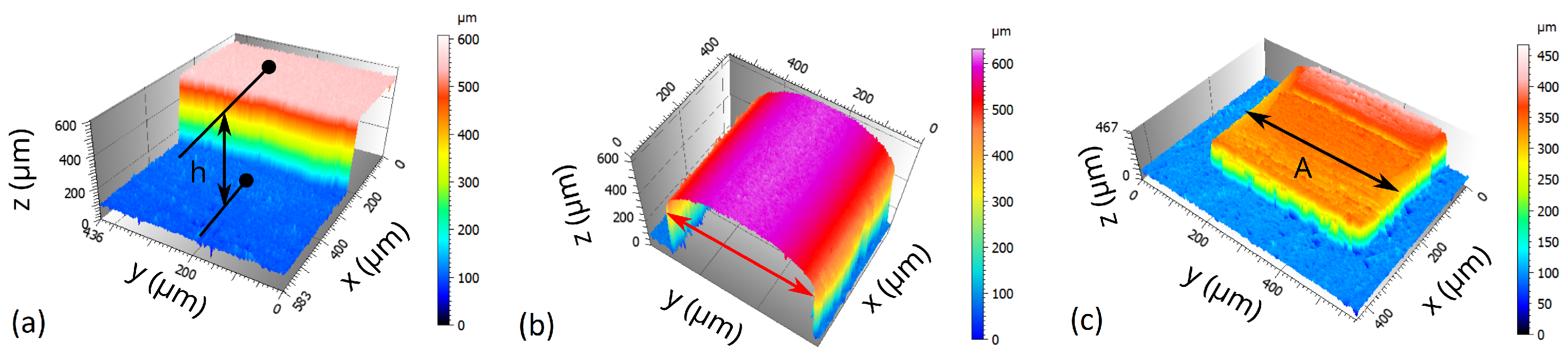
3.3. Measurement Results

To emphasize the advantages of the SATP and further validate its performance, the results obtained without using the proposed SATP for the surface topographies of MAM1 and MAM2 are presented in Figure 7a,b, respectively. Multiple areas with outliers, particularly unexpected protrusions, shown by abrupt color changes, are noticeable. These areas, highlighted by magnified sections (indicated by dashed black arrows in the ‘Top view’ of $xy$-planes), are likely to be deep grooves or regions with steep slopes. The inefficiency of using constant thresholds, indicated by black dashed lines in Figure 7a,b, for removing outliers, is more apparent in the ‘Side view’. Balancing the preservation of valid topography from the removal against the deletion of most outliers is not achievable simultaneously.

Figure 7c,d depict the results after applying SATPs to MAM1 and MAM2, respectively. Unexpected protrusions are absent in both the ‘Top view’ (see magnified section) and ‘Side view’. The trustworthy topographies obtained validate the outstanding performance of the SATP.

The incorrectly reconstructed surfaces result in discrepancies in the determined roughness parameters. The roughness parameters $Sa$ and $Sz$ for Figure 7a–d are listed in

Table 2. Roughness parameters $Sa$ and $Sz$ of samples MAM1 and MAM2 related to the topographies depicted in Figure 7.

	(a)	(b)	(c)	(d)
$Sa$ (µm)	45.3	57.2	44.9	59.3
$Sz$ (µm)	452	543	339	413

(a) to (d), respectively. The deviations in $Sa$ values between (a) and (c) for MAM1 and between (b) and (d) for MAM2 are 0.4 µm and 2.1 µm, respectively. For the $Sz$ values, the deviations are 113 µm and 130 µm for MAM1 and MAM2, respectively. The higher deviations in both $Sa$ and $Sz$ for MAM2 are likely due to its rougher surface. The reduced deviations in $Sz$ are primarily due to the absence of unexpected protrusions and spikes, highlighting the performance and importance of the SATP. Additionally, $Sa$ ≈ 45 µm for MAM1 and $Sa$ ≈ 60 µm for MAM2 indicate that the roughness of these surfaces is quite high. Such roughness levels are typically beyond the capability of common optical surface measuring systems like CSI or CM.

4. Conclusions

This paper details a method for constructing SATPs that effectively prevent artifacts such as unexpected protrusions and spikes. The SATPs are based on results obtained after dual vertical Sobel filtering of the datasets of all planes containing the depth scan direction of an image stack, i.e., the vertical coordinate z. The study also compares the effects of SATPs using different matrix operators, including a horizontal Sobel operator, a Laplacian operator, as well as single and dual vertical Sobel filtering. The proposed method ensures the most accurate reconstruction of surface topographies obtained by FVM.

Moreover, the measured results of the sinusoidal standard Rubert 525C, obtained from both the simulated FVM system and the experimental FVM system, demonstrate consistency. This suggests the potential to validate the FVM system for arbitrary surface textures without requiring deterministic surfaces with sufficient roughness in practice. The results of the proposed method for SATP determination, based on the simulated rough sinusoidal standard, successfully reproduce the sinusoidal shape of Rubert 525C in terms of both amplitude and period.

Additionally, validation was performed on several test pieces with known dimensions, and the corresponding measured results exhibit remarkable consistency, further confirming the effectiveness of the proposed algorithm. Finally, a comparison of measurement results of two different MAM surfaces, obtained with and without SATP, shows that unexpected protrusions and spikes are effectively eliminated in the topographies, providing convincing validation.

References

1. Leach, R. Optical Measurement of Surface Topography; Springer: Berlin/Heidelberg, Germany, 2011; p. 8. [Google Scholar]
2. Safdar, A.; He, H.; Wei, L.; Snis, A.; Paz, L. Effect of process parameters settings and thickness on surface roughness of EBM produced Ti-6Al-4V. Rapid Prototyp. J. 2012, 18, 401–408. [Google Scholar] [CrossRef]
3. Fay, M.F.; de Lega, X.C.; de Groot, P. Measuring high-slope and super-smooth optics with high-dynamic-range coherence scanning interferometry. In Proceedings of the Optical Fabrication and Testing, Kohala Coast, HI, USA, 22–26 June 2014; p. OW1B-3. [Google Scholar]
4. Mirabal, A.; Loza-Hernandez, I.; Clark, C.; Hooks, D.; McBride, M.; Stull, J. Roughness measurements across topographically varied additively manufactured metal surfaces. Addit. Manuf. 2023, 69, 103540. [Google Scholar] [CrossRef]
5. Townsend, A.; Senin, N.; Blunt, L.; Leach, R.; Taylor, J. Surface texture metrology for metal additive manufacturing: A review. Precis. Eng. 2016, 46, 34–47. [Google Scholar] [CrossRef]
6. Król, M.; Dobrzański, L.; Reimann, I. Surface quality in selective laser melting of metal powders. Arch. Mater. Sci. 2013, 88, 88. [Google Scholar]
7. Kerckhofs, G.; Pyka, G.; Moesen, M.; Van Bael, S.; Schrooten, J.; Wevers, M. High-resolution microfocus X-ray computed tomography for 3D surface roughness measurements of additive manufactured porous materials. Adv. Eng. Mater. 2013, 15, 153–158. [Google Scholar] [CrossRef]
8. Fischer, D.; Cheng, K.; Neto, M.; Hall, D.; Bijukumar, D.; Espinoza Orías, A.; Pourzal, R.; Arkel, R.; Mathew, M. Corrosion behavior of selective laser melting (SLM) manufactured Ti6Al4V alloy in saline and BCS solution. J. Bio-Tribo-Corros. 2022, 8, 63. [Google Scholar] [CrossRef]
9. Grimm, T.; Wiora, G.; Witt, G. Characterization of typical surface effects in additive manufacturing with confocal microscopy. Surf. Topogr. Metrol. Prop. 2015, 3, 014001. [Google Scholar] [CrossRef]
10. Newton, L.; Senin, N.; Gomez, C.; Danzl, R.; Helmli, F.; Blunt, L.; Leach, R. Areal topography measurement of metal additive surfaces using focus variation microscopy. Addit. Manuf. 2019, 25, 365–389. [Google Scholar] [CrossRef]
11. Xu, X.; Pahl, T.; Serbes, H.; Lehmann, P. Robust reconstruction of the topography of metal additive surfaces based on focus variation microscopy. In Proceedings of the 60th ISC, Ilmenau Scientific Colloquium, Technische Universität Ilmenau, Ilmenau, Germany, 4–8 September 2023. [Google Scholar]
12. Xu, X.; Hagemeier, S.; Lehmann, P. Outlier elimination in rough surface profilometry with focus variation microscopy. Metrology 2022, 2, 263–273. [Google Scholar] [CrossRef]
13. Xu, X.; Pahl, T.; Serbes, H.; Krooss, P.; Niendorf, T.; Lehmann, P. Preprocessing method for robust topography reconstruction of surfaces of metal additive manufactured parts based on focus variation microscopy. In tm—Technisches Messen; De Gruyter: Vienna, Austria, 2024; Volume 91, pp. 233–242. [Google Scholar]
14. Podulka, P.; Pawlus, P.; Dobrzański, P.; Lenart, A. Spikes removal in surface measurement. J. Phys. Conf. Ser. 2014, 483, 012025. [Google Scholar] [CrossRef]
15. Lou, S.; Jiang, X.; Scott, P. Fast algorithm for morphological filters. J. Phys. Conf. Ser. 2011, 311, 012001. [Google Scholar] [CrossRef]
16. Pan, Y.; Zhao, Q.; Guo, B. On-machine measurement of the grinding wheels’ 3D surface topography using a laser displacement sensor. In Proceedings of the 7th International Symposium on Advanced Optical Manufacturing and Testing Technologies: Advanced Optical Manufacturing Technologies, SPIE, Harbin, China, 26–29 April 2014; Volume 9281, pp. 87–96. [Google Scholar]
17. Lou, S.; Zhu, Z.; Zeng, W.; Majewski, C.; Scott, P.; Jiang, X. Material ratio curve of 3D surface topography of additively manufactured parts: An attempt to characterise open surface pores. Surf. Topogr. Metrol. Prop. 2021, 9, 015029. [Google Scholar] [CrossRef]
18. Giusca, C.; Leach, R.; Helary, F.; Gutauskas, T.; Nimishakavi, L. Calibration of the scales of areal surface topography-measuring instruments: Part 1. Measurement noise and residual flatness. Meas. Sci. Technol. 2012, 23, 035008. [Google Scholar] [CrossRef]
19. Podulka, P. Suppression of the high-frequency errors in surface topography measurements based on comparison of various spline filtering methods. Materials 2021, 14, 5096. [Google Scholar] [CrossRef] [PubMed]
20. Bitenc, M.; Kieffer, D.; Khoshelham, K. Range versus surface denoising of terrestrial laser scanning data for rock discontinuity roughness estimation. Rock Mech. Rock Eng. 2019, 52, 3103–3117. [Google Scholar] [CrossRef]
21. Pahl, T.; Rosenthal, F.; Breidenbach, J.; Danzglock, C.; Hagemeier, S.; Xu, X.; Künne, M.; Lehmann, P. Electromagnetic modeling of interference, confocal, and focus variation microscopy. Adv. Photon. Nexus 2024, 3, 016013. [Google Scholar] [CrossRef]
22. Pawlus, P.; Reizer, R.; Wieczorowski, M. Comparison of results of surface texture measurement obtained with stylus methods and optical methods. Metrol. Meas. Syst. 2018, 25, 589–602. [Google Scholar] [CrossRef]
23. Lou, S.; Jiang, X.; Sun, W.; Zeng, W.; Pagani, L.; Scott, P. Characterisation methods for powder bed fusion processed surface topography. Precis. Eng. 2019, 57, 1–15. [Google Scholar] [CrossRef]
24. Burger, W.; Burge, M.J. Digital Image Processing: An Algorithmic Introduction; Springer Nature: Cham, Switzerland, 2022. [Google Scholar]
25. Subbarao, M.; Choi, T. Accurate recovery of three-dimensional shape from image focus. IEEE Trans. Pattern Anal. Mach. Intell. 1995, 17, 266–274. [Google Scholar] [CrossRef]
26. Nwaogu, U.; Tiedje, N.; Hansen, H. A non-contact 3D method to characterize the surface roughness of castings. J. Mater. Process. Technol. 2013, 213, 59–68. [Google Scholar] [CrossRef]
27. ISO 25178-601:2010; Geometric Product Specifications (GPS)—Surface Texture: Areal—Nominal Characteristics of Contact (Stylus) Instruments. International Organization for Standardization: Geneva, Switzerland, 2010.
28. ISO 25178-2:2012; Geometric Product Specifications (GPS)—Surface Texture: Areal—Part 2: Terms, Definitions and Surface Texture Parameters. International Organization for Standardization: Geneva, Switzerland, 2012.
29. Hagemeier, S.; Schake, M.; Lehmann, P. Sensor characterization by comparative measurements using a multi-sensor measuring system. J. Sens. Sens. Syst. 2019, 8, 111–121. [Google Scholar] [CrossRef]
30. Hagemeier, S. Comparison and Investigation of Various Topography Sensors Using a Multisensor Measuring System. Ph.D. Thesis, University of Kassel, Kassel, Germany, 2022. [Google Scholar]
Figure 1. Validation samples of (a) Rubert 525C standard, (b) an electrical resistor on an aluminum baseplate, (c) a drill, and (d) an optically-coupled logic gate as well as two MAM samples: MAM1 (e) and MAM2 (f).
Photonics 11 01011 g001
Figure 2. Flowchart illustrating the complete procedure devised for the construction of the SATP.
Photonics 11 01011 g002
Figure 3. Illustration of the proposed method by using a dataset belonging to MAM2: (a) x z -plane on a cross section of an image stack; (b) reconstructed profile without using SATPs applied to the cross section depicted in (a); (c) intensities extracted from (b) marked by dashed white line; (d) the result after applying once the vertical Sobel operator on (a); (e) the result after applying once the horizontal Sobel operator on (a); (f) the result after applying the Laplacian operator on (a); (g) the result after applying twice the vertical Sobel operator on (a); (h) normalized absolute values extracted from (g) with respect to the dashed white line; (i) a result after applying a moving average filter (with window size of 50 samples) to (g); (j) evaluated profile using the proposed method applied to the cross section shown in (a). x-column is changed into z-column in the figure.
Photonics 11 01011 g003
Figure 4. (a) pairs of upper (blue curve) and lower (orange curve) limits calculated based on Figure 3g; (b) linearly interpolated upper and lower limits based on (a); (c) pairs of upper and lower limits calculated by applying once the vertical Sobel operator; (d) pairs of upper and lower limits calculated by applying a Laplacian operator.
Photonics 11 01011 g004
Figure 5. Comparison of a cross section in the x z -plane of an image stack obtained by (a) simulation and (b) measurement for the sinusoidal standard Rubert 525C. (c) Simulation result after adding a roughness topography with R a value of 200 nm to the sinusoidal texture. (d) The simulation result shown in (c) is superposed with the reconstructed profile (green line) after using the proposed SATPs.
Photonics 11 01011 g005
Figure 6. Reconstructed topographies of validation specimens shown in Figure 1b–d: (a) section of an SMD resistor of height h, (b) the shaft of a drill, and (c) section of a solder foot of an optically-coupled logic gate IC.
Photonics 11 01011 g006
Figure 7. Reconstructed topographies of MAM1 (a,c) and MAM2 (b,d) before using SATPs (a,b) and after using SATPs (c,d).
Photonics 11 01011 g007