A Linear, Direct Far-Field Subwavelength Imaging Method: Microparticle-Assisted Nanoscopy

Abstract

Microparticle-assisted nanoscopy (MAN) is a novel emerging technique of direct far-field deeply subwavelength imaging, which has been developed since 2011 as a set of experimental techniques. For a decade, the capability of a simple glass microsphere without fluorescent labels or plasmonic elements to grant a direct, broadband, deeply subwavelength image of a nanostructured object was unexplained. Four years ago, the explanation of MAN via the suppression of diffraction was suggested by the author of the present overview. This explanation was confirmed by extensive full-wave simulations, which agreed with available experimental data and revealed new opportunities for MAN. Although the main goal of the present paper is to review recent works, state-of-the-art concepts in MAN are also reviewed. Moreover, so that the peculiarities of MAN are better outlined, its uniqueness compared to other practically important methods of far-field subwavelength imaging is also discussed.

1. Introduction

In the XIX century, Ernst Abbe considered in [1] the problem of ultimate spatial resolution granted by a microscope to a grating of point scatterers with a small period $\delta$ between them. Due to the diffraction caused by the microscope objective lens, the minimal resolved gap between the scatterers turned out to be finite and equal to the effective radius of the so-called Airy disk, i.e., the spot of intensity in the image plane granted by the same lens to a point dipole. This spot, resulting from the diffraction of the dipole radiation by a thin lens, was previously studied by G.B. Airy in [2]. Later, the results of [1] were revised in work by Lord Rayleigh [3], who, instead of a grating illuminated by a plane wave, considered a pair of point dipole sources. Rayleigh deduced that the ultimate resolution ${\delta }_{\min }$ equals the radius of the Airy disk $0.61\lambda /nsin\psi$ (Abbe’s result for his grating) when two dipoles radiate in phases. Here, n is the refractive index of the medium filling in the space between the object and the microscope (usually, it is free space, i.e., $n=1$), and $\psi$ is the angle between two straight lines connecting the center of the dipole pair with the center of the objective lens and with its edge, respectively. If two dipoles are not mutually coherent, the ultimate resolution is slightly finer than the Airy disk radius: ${\delta }_{\min }=\lambda /2nsin\psi$. Rayleigh’s results can be considered a slight correction of [1] and can also be referred to as the Abbe ultimate resolution [4].

If the objective lens with a large aperture is located at a small distance from a microscopic object, one may assume $\psi \approx \pi /2$. Then, we come to the ultimate resolution of two non-coherent scattering points ${\delta }_{\min }=\lambda /2$ and to that of two in-phase scattering points $0.61\lambda \approx 0.6\lambda$. One often unites these two results and calls the interval ${\delta }_{\min }$ = (0.5–0.6)$\lambda$ the Abbe diffraction limit. Some modern authors refer to this estimate for ${\delta }_{\min }$ as the Rayleigh diffraction limit (see, e.g., [5,6,7]). The Abbe limit (below, we will use this name) was originally deduced for a particular imaging system that was electromagnetically linear and did not comprise other bodies but the object and the microscope located in the far zone of the object. It is implied that the image was visualized directly, without post-processing of the recorded intensity distribution. It was clear that the Abbe limit (0.5–0.6)$\lambda$ was deduced for two scenarios of object illumination in a particular imaging system. However, the optical community treated this particular result as a fundamental limit of the resolution caused by diffraction (see, e.g., [4]). Was this a simple misunderstanding?

No, it was not. The logic of opticians believing in the fundamental nature of the Abbe limit was as follows. A direct acquisition of a far-field image of a tiny object obviously demands its magnification, which can only be achieved through a lens. Therefore, any direct imaging system must comprise a lens. If we consider the spatial spectrum of the far field produced by the object, the lens acts as a low-pass filter for spatial frequencies (components of the wave vector $\mathbf{k}$ orthogonal to the optical axis of the imaging system). Large spatial frequencies (i.e., plane waves strongly tilted to the axis) are scattered by the lens in lateral directions and do not contribute to the image; therefore, the lens worsens the optical signal and puts a limit on the resolution. This resolution (0.5–0.6)$\lambda$ is achievable only for the simplest imaging system, which was considered by Airy, Abbe, and Rayleigh. The presence of additional bodies near the object may only worsen the ultimate resolution since any body produces an additional diffraction, especially if the body is located near the object [8]. This insight can be referred to as the conventional paradigm of direct optical imaging.

The rise of scanning near-field optical microscopy (SNOM) in the 1970s stimulated the scientific community to recall that the Abbe diffraction limit makes no sense in near fields [9]. In SNOM, images with a resolution of ${\delta }_{\min }<\lambda /2$ (usually called super-resolution) result from the scanning of a cantilever tip of subwavelength thickness, which either collects or emits photons. In the first case, the tip transfers the optical signal created by a subwavelength part of the object to the receiver. In the second case, the tip excites a subwavelength part of the object, and the scattering of this part is measured in the far zone. In both cases, the imaged part of the object is distanced maximally by dozens of nm from the apex of the tip [10]. Therefore, the field involved in SNOM imaging is the so-called near field, in which evanescent waves dominate over the propagating waves. Super-resolution in SNOM does not contradict the opinion that the Abbe limit obviously holds in linear, direct far-field optical imaging.

This point of view was shared by John B. Pendry, who suggested in [11] that the Abbe limit in the far zone of the object should be beaten by transmitting the near fields there. In that paper, it was proven that the evanescent spatial spectrum of the near field around a point source could be exactly reproduced at an optically substantial distance using the so-called Veselago pseudo-lens. The Veselago pseudo-lens is a layer of a hypothetical medium, the so-called left-handed metamaterial, whose relative permittivity $\epsilon$ and permeability $\mathsf{\mu }$ are both equal to $-1$. V.G. Veselago showed in [12] that such a layer should focus without aberrations on rays diverging from a point source into a point located at the same distance from its rear interface as the distance between the source and front interface. In accordance with [11], the evanescent waves existing around the point source are transferred by this layer at the same image point without distortions because they are uniformly amplified across the layer, and this amplification exactly compensates for their decay in free space. So, the ray image and the near-field image occur at the same point, and the Veselago pseudo-lens turns out to be a perfect lens, granting the perfect image of a point source [11].

Since 2000, all attempts to validate this claim numerically and check it experimentally have failed for two reasons. First, the target values $\epsilon =\mathsf{\mu }=-1$ for evanescent waves are not achievable in principle due to the unavoidable granularity of the metamaterial and electromagnetic loss. Meanwhile, even small deviations from the target values are critical for the subwavelength resolution. Second, it was theoretically shown that perfect imaging implies singularity: infinite reactive power stored in a metamaterial layer. The detection of such a singular image would demand the full absorption of the light at the image point. In a continuous absorber, such as a sheet of photoresist, the image of a luminescent point cannot be point-wise and cannot even be a subwavelength spot. The necessity of absorption makes further research in this area impossible. More details on this issue and relevant references can be found in [13].

However, [11] played a great positive role in the development of imaging. First, it attracted the attention of researchers to metamaterials, i.e., effectively continuous composites with unusual and useful optical properties. Scientists studying metamaterials created a class of novel imaging structures called magnifying metamaterial superlenses or hyperlenses [14,15,16]. Although these structures were expensive and challenging to fabricate, they granted the linear, direct image in the far zone of the object together with object magnification. They allowed one to see and record the subwavelength details of the objects (see, e.g., [13,17]). Second, besides the idea of the perfect lens, [11] also comprised the idea of the so-called poor man’s superlens (PMSL). PMSL is simply a submicron-thick nanopolished layer of silver. This layer is thicker than the skin-depth of silver, i.e., it is practically impenetrable for propagating waves, but at the wavelength of the so-called plasmon resonance, the TM-polarized evanescent waves created by a closely located object are uniformly amplified across it. This uniform amplification results in the transfer of the near field image through the PMSL and grants the ultimate resolution of the order of ${\delta }_{\min }$ = (0.2–0.3)$\lambda$ to a scanning probe located behind the layer at the same distances. This idea offers the beneficial decoupling of the scanning probe of an SNOM from the object (in the usual SNOM, their coupling is often destructive for the object). Moreover, the PMSL was successfully applied for the commercial replication of ultraviolet diffraction gratings (see, e.g., [13]).

Abundant investments in nanotechnologies in the early 2000s stimulated the rise of other far-field imaging methods for which the Abbe diffraction limit is not applicable. In some of these methods, a microscope is used, but either nonlinear or parametric photonic processes are involved, which disable the Abbe limit, such as Raman scattering by the object surface and fluorescence from it. In 1994, the imaging method utilizing fluorescent labels (organic dye molecules or quantum dots) covering the object in combination with the so-called confocal dark-field microscope was suggested in [18]. In the 2000s, this method was called stimulated emission depletion (StED) imaging and has been practically developed so well that the ultimate lateral resolution ${\delta }_{\min }\approx \lambda /20$ was achieved. In 2014, its main authors (E. Betzig, S. Hell, and W. Moerner) were awarded a Nobel Prize.

In addition to StED, several methods granting super-resolution due to fluorescent labels covering the object have been developed. Among them, the reversible saturated fluorescence transition method, photo-activation localization method, and saturated structured illumination method have granted resolution of the order of ${\delta }_{\min }$∼$\lambda /10$ (see, e.g., [19]).

Meanwhile, linear optical imaging (without nonlinear labels) still remains of prime importance for biomedical investigations. Far-field label-free subwavelength imaging (LFSI) does not demand the introduction of labels, which may cause harm to the object. LFSI is implied as linear imaging, which introduces no restrictions to biomedical applications in which the sub-cellular structures are directly visualized in vivo. All of the known methods of LFSI are reviewed below. Here, we will prove that the Abbe limit is not applicable to them.

The general drawback of LFSI is subtle scattering in cases when the nanostructured object is not resonant. It results in rather low image contrasts compared to the images obtained with the use of nonlinear physical processes. This low contrast makes the problem of super-resolution tightly related to the problem of the limited photon budgets offered by unstained nanostructured objects. Both of these problems are resolved in smart LFSI methods via a sufficient set of optical measurements and their post-processing. The accumulation of measured data allows one to reimburse the lack of contrast, and one obtains a reliable image of a weakly scattering object with super-resolution. However, it is achieved by the price of the finite time resolution. Really, if the image is visualized on the display after post-processing of the measured data, a certain amount of time is required for this visualization. This time delay may not be convenient for the imaging of moving or transforming objects.

A direct method of LFSI was suggested in 2011 in [20]. This work revealed the capability of a simple glass microsphere to offer the far-field lateral super-resolution of flat nanostructured objects. A set of such objects was located in a tiny crevice formed by the nanostructured substrate and the microsphere touching the substrate at a point of rest. The object was illuminated by a laser light with variable frequency. The spheres studied in [20] had radii in the limits R = (2–9)$\lambda$ and refractive indices of $n=1.46,1.8$ and 2. These spheres offered super-resolution in all cases under study. Of course, the microscope cannot resolve subwavelength details without magnification; its objective lens forms an image of a virtual object created by the sphere, in which the real object is magnified M times. This virtual object is located behind the real object in the substrate. A resolution of $\lambda /8$ was achieved in cases where the magnification was as high as M = 7–8.

The authors of [20] claimed that these virtual objects were the same as those predicted by geometrical optics (GOs) in all cases, as the microspheres were usual macroscopic lenses of spherical shape. Since it is commonly believed that GOs have no predictive power for this case (the distance d between the object and the lens is smaller than $\lambda$, and the lens size is comparable with $\lambda$) due to diffraction, the reason for the correct prediction of M by the GO was not explained in [20].

This amazing method of imaging is called microsphere-assisted nanoscopy (MAN) or microsphere-assisted microscopy (MAM). It has been extended to microcylinders (microfibers), which grant 1D super-resolution and 1D magnification [21,22,23]. Nowadays, the abbreviation MAN can be understood as microparticle-assisted nanoscopy, implying that both glass microsphere and microfiber are microparticles (MPs). Experiments have shown that the 1D ultimate resolution offered by glass microfiber is nearly the same as the 2D lateral resolution granted by a glass microsphere, although the magnification is lower (M = 2–3 versus 3–10 granted by the spheres in the known experiments). Over the past decade, works about MAN have formed a body of literature, and the main achievements of MAN are reviewed almost annually, e.g., in [17,21,23,24,25,26,27,28,29].

Two different names (MAN and MAM) are utilized in the literature for the same method of LFSI and can be explained as follows. Optical imaging in visible light is usually referred to as nanoscopy (or nanoimaging) if the resolution is below 100 nm. It corresponds to the case when the resolution is as fine as ${\delta }_{\min }$∼$\lambda /10$ or finer. The super-resolution $\lambda /4<{\delta }_{\min }<\lambda /2$ is referred to as slightly subwavelength. Corresponding imaging techniques are usually referred to as subwavelength optical microscopy. Glass MPs (microfibers and microspheres) may offer either slight or deep super-resolution depending on their parameters and those of the substrate. Therefore, both MAN and MAM can be used equally for this imaging method. Below, only the name MAN is used for certainty. It is probable that the main practical achievement of MAN is two techniques that allow one to image all tiny objects in a macroscopic area via the displacement of MPs over the substrate [21,22]. Another important achievement results from the combination of a glass MP with the so-called Mirau interferometer. In this way, one can achieve a 3D deep super-resolution for bulk nanostructured objects [30].

However, during the first decade after the publication of [20], optical theorists suggested only a few very particular and not very convincing explanations of MAN. Most of the experimental results remained unexplained until 2020, when a hypothesis of the underlying physics of MAN was suggested by the author of the present overview in [31]. This hypothesis was based on the dipole source pattern having the exact zero on the dipole axis. Due to this feature, the diffraction effects are suppressed for a radially (with respect to the MP) polarized dipole in the paraxial region of the wave beam created by this dipole behind the MP. This suppression makes the GO applicable, and the magnification granted by the MP can be correctly explained in terms of rays. The main goal of the current overview is to present the main theoretical results confirming this hypothesis. However, to better elucidate the unique features of MAN, the author felt it was necessary to show its place in the set of known LFSI methods. Therefore, practical achievements of all LFSI methods, not only those of MAN, are reviewed below. This review is educational and strongly differs from the review of LFSI presented in the recent roadmap article [19]. At the end of the present paper, three main action points which may revolutionize MAN are formulated.

2. Label-Free Subwavelength Imaging

2.1. List of Indirect Label-Free Subwavelength Imaging Techniques

There are several methods of linear optical imaging in far fields for which the limit $\lambda /2sin\psi$ related to the lens is irrelevant simply because the image is formed after a set of optical and post-processing measurements. All these indirect imaging methods are mentioned in [19]. Among them, there are methods which, in accordance with the above definition of nanoscopy, should be referred to as nanoscopic, although the original names of these methods do not contain the word “nano”:

• Ultramicroscopy [32,33];
• Diffraction grating-assisted microscopy (Lukosz microscopy) [34,35,36];
• Computational imaging using machine learning [37];
• Computational imaging using compressed optical sensing [38];
• Sparsity-based diffraction imaging, including tomographic diffraction imaging [39,40,41];
• Nanoimaging based on the interferometric detection of scattering (iSCAT) [42,43];
• Topological microscopy [44,45].

These methods are united in [19] by the name of an informational approach to far-field nanoscopy. In the present paper, another name is suggested for these methods: smart optical nanoscopy.

LFSI methods with post-processing in which the experimentally reported ultimate resolution is slightly subwavelength are as follows:

• Structured illumination microscopy without fluorescent labels (Gustafsson microscopy) [46];
• Far-field phase-contrast microscopy (Zernike microscopy) [47];
• Differential interference contrast microscopy (Hoffman microscopy) [48];
• Digital holographic microscopy [49];
• Computational integral imaging [50];
• Quantitative phase imaging [51].

Each of these methods is targeted to specific chemical, biological, or biomedical applications and implies a finite time resolution. The methods listed in this subsection are discussed below in their historical context.

2.2. Prehistory of LFSI

In 1903, R. Zsigmondy and H. Siedentopf analyzed the spectra of Tindall scattering, i.e., the lateral scattering of visible light by substantial nanoparticles of size 400–500 nm uniformly distributed (due to Brownian movement) in a colloidal solution. Additionally, on a photographic plate, they recorded the intensity distribution of the laterally scattered light. Combining these data, they managed to retrieve both the frequency-dependent polarizability of an individual particle and their concentration in water. In other words, they indirectly measured the mean inter-particle distance a in a colloid. This method turned out to be applicable even if this distance was smaller than the wavelength, which was a breakthrough at that time [32]. Further development of this method, called ultramicroscopy by its authors, allowed the extension of the method to Rayleigh scattering, i.e., deeply subwavelength colloidal nanoparticles and optically dense colloids in which $a<\lambda /2$. This achievement in ultimate resolution was awarded the Nobel Prize in 1925. Nowadays, ultramicroscopy is a widely used technique of biomedical sensing, and even a multidisciplinary journal with the same name exists. In the modern version of this method, the distribution of intensity is recorded by advanced optical detectors, in which the spectral analysis is also advanced, and arrays a as small as a few dozen nm are measured [33]. Indeed, these achievements do not dispute the Abbe limit because an array of particles is not truly imaged. Only the mean parameters are indirectly measured, and only the time-averaged nanostructure of the array is retrieved. However, ultramicroscopy is an important stage of the prehistory of LFSI.

In 1934, F. Zernike (Nobel Prize in 1953) suggested a method for image retrieval using structured illumination, which increased image contrast/visibility and reduced the impact of diffraction by a lens. This method, called phase contrast microscopy, was developed extensively and, in the 1960s, allowed one to restore recorded images with a resolution below $\lambda /2sin\psi$ without immersion [47]. The effective enhancement of the numerical aperture compared to $sin\psi$ occurs due to the coherent illumination created with an interferometer. Since, in this method, $sin\psi \ll 1$, the improvement of the resolution was not sufficient enough to beat the half-wavelength limit. Therefore, this achievement also refers to the prehistory of LFSI.

In 1952, G. Toraldo di Francia [52] pointed out a link between far-field super-resolution in optics and the phenomenon of superdirectivity in phased antenna arrays at microwaves. Superdirectivity (also called supergain) is a highly directive pattern of a phased antenna array whose overall size is below $\lambda /2$. Antennas of a superdirective array separated by a deeply subwavelength gap $\delta$ can be resolved in their far field because the array pattern for specially engineered phases keeps the information of both $\delta$ and phase shifts between the dipole moments of antennas. The author of [52] noticed that in optics, there may be situations when the far-field pattern of the object keeps the information of its subwavelength structure. Then, the image beating the Abbe limit may be retrieved from the measured far-field intensity pattern. Indeed, this work also refers to the prehistory of LFSI.

2.3. Indirect LFSI Methods

In 1966, W. Lukosz, in his pioneering work [34], raised the question of the ultimate resolution in the case of if an image created by a lens is recorded several times for different cases of illumination and its post-processing is allowed. Lukosz explained why, in this case, the Abbe diffraction limit is not relevant. Using the apparatus of Fourier optics, he proved that the ratio ${\delta }_{\min }/\lambda$ depends on the composition of the imaging system, and its finite value results from the restricted information capacity of this system. In the same work, several ways to indirect super-resolution were suggested: the use of pinholes for the illumination of the object and for the formation of its image, the use of two orthogonal polarizations of the incident light, and the use of phase diffraction gratings.

The last suggested method promised a deeply subwavelength image along one transverse Cartesian axis (e.g., z), sacrificing the lateral resolution along the other transverse axis (e.g., x). In the tangential object plane, the spatial spectrum of the object near field (i.e., the effective interval of the wave vector components $(k_x,k_z)$) should be effectively shrunk along the $k_z$ axis, utilizing phase diffraction grating with period $b>\lambda$ located in the near vicinity of the object. When evanescent waves propagating along z, i.e., waves with $k_z>k_0$ and imaginary $k_y$ (here $k_0=\omega /c$), are in the spatial resonance with some Floquet harmonics of the field scattered by the grating (i.e., with plane waves having the z-component of the wave vector $k_z^{\prime }=2\pi m/b\pm k_z$, where $m=\pm 1,\pm 2,\dots$), these evanescent waves are converted into propagating plane waves ($|k_z^{\prime }|<k_0$) by the grating. If we know the approximate distances between the partial nanoscatterers forming the object, we may estimate the dominant spatial frequencies in the spatial spectrum of the object and find the set of m. Corresponding plane waves should carry the information of deeply subwavelength details of the object. In this model, Lukosz utilized the property of the phase diffraction gratings to share the dominant Floquet harmonics out from the scattering spectrum.

The Lukosz method demanded that the distance d between the object and the grating would be deeply subwavelength and that the grating would be fabricated with nanometer precision. In the 2000s, the development of nanotechnologies granted the needed precision, and in 2006 the Lukosz method was ingeniously implemented in work [36] where the transmitting phase-diffraction grating was combined with the poor man’s superlens suggested by Pendry.

The first drawback of this method was the necessity of some prior knowledge of the object’s internal structure. The second drawback was the negligence of optical noises. Therefore, this work could not be used to obtain the explicit limit for the ultimate resolution, and in 1986, this approach was revisited in [35], where optical noises were qualitatively taken into account. However, in [35], the problem remained unsolved: no explicit expressions for the ultimate resolution restricted by noises were deduced. The goals of [35] were to explain why the Abbe limit is irrelevant for imaging systems with post-processing and to show that the ultimate resolution of such systems is determined not only by the information capacity of the imaging system but also by the signal-to-noise ratio (SNR) in the object area. The explicit expression for ${\delta }_{\min }$ of a flat nanostructured object taking SNR into account was deduced much later in [53]:

$${\delta }_{\min }={\displaystyle \frac{\lambda /2}{{log}_2\sqrt{1+2SNR+\zeta SN{R}^2}+O(1/k_{0}L)}}$$

(1)

In (1), $SNR$ is the mean signal-to-noise ratio in the area of the signal detectors, which also takes their own noises into account, $\zeta$ is the integral coefficient depending on the distribution of the complex permittivity inside the object, and L is the object transverse size. Formula (1), which was derived under assumption $k_{0}L\gg 1$, is not applicable to such an object as a pair of dipoles with a subwavelength gap between them. As to the coefficient $\zeta$, it may be arbitrary, but it was shown that it is close to unity when the object consists of alternating transparent and opaque parts (e.g., an array of metallic nanoparticles in a dielectric host) and vanishes if the object is lossless (e.g., an array of dielectric nanoparticles in the free space of another dielectric host). For these two cases, assuming $SNR\gg 1$, one may deduce the following from (1):

$${\delta }_{\min }^{lossl.}\approx {\displaystyle \frac{\lambda }{1+{log}_{2}SNR}},{\delta }_{\min }^{opaque}\approx {\displaystyle \frac{\lambda }{2{log}_{2}SNR}}$$

(2)

In accordance with [35], dark-field microscopy grants the signal-to-noise ratio as high as $SNR$∼${10}^3$–${10}^4$. For dark-field microscopy with post-processing of recorded images, Formula (2) implies ${\delta }_{\min }=(\lambda /10-\lambda /15)$ for lossless objects and ${\delta }_{\min }=\lambda /20-\lambda /30$ for objects composed of opaque (metal) nanoblocks.

Restrictions to (2) are not relevant for nonlinear and parametric methods of imaging. They are also not applicable to the case when prior knowledge about the object is used. Finally, the derivation of this limit in [53] refers to illumination by a wave beam and does not cover the case when the incident light is nanostructured (for example, when it contains evanescent waves).

In 1999, a linear indirect LFSI method called structured illumination microscopy (SIM) was suggested by M. Gustafsson. SIM, described in [46], grants the modest ultimate resolution of $0.31\lambda$, but its advantage is that prior knowledge about the object is not required. In this technique, one illuminates the object laterally with a laser light using a mirror, creating a standing wave. The images should be recorded for a sufficient amount of illumination in different lateral directions. A set of intensity distributions corresponding to a set of standing waves recorded in the image plane of a microscope grants the object image in which the spatial resolution is twice as fine as ${\delta }_{\min }\approx 0.6\lambda$, i.e., the Abbe limit for two mutually coherent sources.

In the 2000s, the SIM method was modified using the fluorescent molecules attached to the surface of the object. Since they emitted light at mutually random phases, it allowed one to enhance the resolution to $0.25\lambda$. Further, one developed a related method, which was called SIM with saturated fluorescence or simply saturated SIM. This method, in combination with the metamaterial substrate of an object, offered the ultimate resolution $\lambda /12$ [54]. However, this story goes beyond the framework of LFSI.

The method of indirect imaging based on machine learning, the method based on compressed sensing, and the method based on so-called optical signal sparsity were developed in the 2000s. All of them grant the ultimate resolution of the order of $\lambda /10$ without prior knowledge about the object. These three methods are three different types of coherent diffraction imaging, an approach in which the intensity of light scattered by the object is measured in a sufficiently wide sheer of angles, and the image is retrieved using a specific post-processing algorithm. Not only are these algorithms different in these three methods, but they also differ by the regions in which the scattering is measured (forward scattering, backward scattering, and lateral scattering) and by the schemes of the object illuminations.

The method based on the optical signal sparsity seems advantageous compared to two of its counterparts. Only one measurement is sufficient for this method, which makes its time resolution the finest one. The corresponding post-processing exploits the fact that the far field produced by an array of nanoscatterers illuminated by a plane wave is a set of mutually coherent spherical waves with slightly different amplitudes and phase centers. This fact is treated as the sparsity of the far-field pattern.

Sparsity in the theory of signals is defined as the smallness of the most projections of a signal function onto a complete set of properly chosen base functions. For this method, sparsity means that the far-field pattern of a nearly planar nanostructured object is an expansion over a finite functional basis in which a finite number of the base functions (spherical waves) are significant. The spatial filtering operation applied to the measured intensity distribution allows one to retrieve these base functions (amplitudes and phases) from the result of their interference. These functions accurately point out the locations of the nanoscatterers composing the object and allow us to retrieve their polarizabilities [40]. In [39], an image with a resolution of $\delta \approx \lambda /8$ was restored experimentally for a pair of nanoparticles. In further works, the same resolution was achieved for more complex objects.

An important indirect method of LFSI is the method called iSCAT, which was developed in the 1990s. It is similar to ultramicroscopy in the sense that it does not grant the true image but some statistical data about the inter-particle distances. In this method, the resolution limit (2) is not applicable because the method implies prior knowledge about the nanoparticles forming the object. Namely, this method is applicable only to nanoparticles whose polarizabilities are known. The measurements of array scattering after post-processing deliver both the mean gap between these particles and the statistical deviation of this gap. Nowadays, this method grants an amazing resolution for this gap of the order of $\lambda /100$ [42]. The post-processing of the iSCAT method is very fast, and iSCAT is applicable even for rapidly moving nanoparticles [43].

The method called topological microscopy does not demand any prior knowledge of the object, although it grants a similarly amazing ultimate resolution. This method is based on so-called superoscillatory illuminations of an object [45]. Superoscillation in LFSI is defined as a small-scale variation of the amplitude and phase of the incident light in the object plane. The scale of this variation is subwavelength without evanescent waves, which is possible due to specially engineered interference of propagating spatial harmonics [55]. Such interference resulted in works [44,45] from the transmission of a plane wave through a thin spatially modulated nanolayer, which can be referred to as a periodically non-uniform metasurface. The superoscillatory spatial distribution of the incident light was called topologically structured illumination in [44] because it was determined by the topology of the metasurface. In [44], it was experimentally shown that a set of topological illuminations with different patterns in combination with artificial intelligence may grant the lateral resolution of flat nanostructured objects as fine as ${\delta }_{\min }\approx \lambda /130$ and sometimes even ${\delta }_{\min }\approx \lambda /200$. The limit (2) is not applicable to topological microscopy because the superoscillatory illumination of the object is nanostructured. The main drawback of topological microscopy is quite long post-processing that practically restricts its applicability to static objects.

It is interesting that the name topological nanoscopy was later attributed to one of the techniques of near-field scanning microscopy, namely, the method utilizing the so-called Ebbesen effect of extraordinary optical transmission [56]. The fact that topological microscopy [44] grants much finer resolution than ${\delta }_{\min }=\lambda /70$ granted by the topological nanoscopy [56] is an illustration of the terminological mess found in modern optical literature.

After learning the achievements of smart optical nanoscopy, a reader not working in this area should be hardly motivated to familiarize themselves with such methods of LFSI as differential interference contrast microscopy, digital holographic microscopy, computational integral imaging, and quantitative phase imaging. As noticed above, these methods also demand post-processing and offer a slightly subwavelength resolution. Their importance is related to the specific advantages of these methods for targeted applications.

For the completeness of this review, it is reasonable to mention so-called advanced solid immersion lens microscopy. Although it grants resolution of $0.15\lambda$ [57], after some post-processing (reconstruction of the refractive index spatial distribution in the object area), it is not nanoscopy. It is a technique of far-infrared imaging, and the best resolution achieved is of the order of several microns.

To sum up, the ultimate resolution in smart nanoscopy is not limited by lens diffraction either due to the absence of lenses or due to the post-processing of the image recorded using lenses. Post-processing makes the conventional paradigm of optical imaging irrelevant and does not touch the Abbe limit. This paradigm and this limit are disputed by other imaging methods, such as those reviewed below.

2.4. Far-Field Surface Plasmon Resonance Microscopy

The conventional paradigm of direct optical imaging was first disputed by Richard Feynman. In 1963, Feynman read the course of general physics to his students, which was recorded by them by hand, and after Feynman’s death, it was published as a study book [58]. Feynman caught the attention of his students with the fact that the Abbe diffraction limit refers to the case when the object scatters the light in a steady regime. Therefore, an aperiodic time-varying illumination will disable this limit. Here, we do not concern ourselves with the story of high-resolution imaging in time-varying systems. Instead, we formulate the following question: can the Abbe limit be beaten for a steady regime in a linear, direct image formed by the objective lens of a usual microscope? The answer is yes. To the knowledge of the author, this answer was first given in 2005 by I. Smolyaninov, who suggested so-called far-field surface plasmon resonance microscopy (FF SPRM).

In [59], the previously known method of surface-plasmon resonance microscopy (SPRM) was modified and became a far-field LFSI method. Initially, SPRM was one of the SNOM techniques used for sensing dielectric nanolayers and measuring their thicknesses [60]. Whereas a usual SNOM grants a subwavelength image of a flat object with a resolution of 40–50 nm, SPRM allows one to measure the thickness of dielectric nanoobjects with excellent precision (1 nm or even less). This technique utilizes the unique property of an interface between a nanopolished plasmonic metal (silver or gold) and dielectric. Along such an interface, a surface wave called surface plasmon polariton (SPP) may propagate in the range of visible light. The wavelength of the SPP shortens compared to $\lambda$ up to ${10}^3$ times, and this shortening depends on the dielectric thickness.

In [59], the imaging system utilizing the SPP comprised not a flat dielectric microparticle or a multilayer structure on top of a plasmonic metal as in the usual SPRM method but a macroscopic droplet of liquid dielectric (glycerine) with a specially adjusted shape resembling a pear, as shown in Figure 1. An SPP on the interface metal/glycerine is excited by a laser beam obliquely incident through a prism and impinges on the object located on the metal surface in the narrow part of the droplet (around its internal focus). If this object is an array of nanoscatterers, every nanoscatterer acts as a point dipole, partially converting the incident SPP into a scattered SPP. This SPP has a circular front and propagates from the dipole in all directions. It totally (internally) reflects from the boundary between the glycerine and the air because, at the operation frequency, the SPP cannot exist on the boundary metal/air. As a result, the droplet focuses the scattered SPP produced by a nanoparticle into a hot spot of electromagnetic field located in the wide part of the droplet. Since the object (called the “sample” in [59]) is located in the narrow part of the droplet, and the corresponding array of hot spots is located in its wide part, the gaps between these spots are magnified. Every hot spot, referred to as [59] in the intermediate image, has the horizontal dipole moment shown in Figure 1 by an arrow. Really, the subwavelength concentration of the electric field on the metal surface is the same as the subwavelength concentration of the surface current, which is the same as the Hertzian dipole. These dipoles (virtual sources, in the terminology of the present paper) correspond to every nanoparticle forming the object. In a properly shaped droplet, the gaps between the virtual sources (VSs) may be magnified by an order of magnitude. This effect was referred to as [59] in the in-plane magnification.

Indeed, both the primary source (nanoscatterer) and corresponding VSs, being the dipole light sources, create bulk spherical waves propagating in the glycerine towards its top surface. These waves transmit into free space and are developed by the microscope. The wave beams leaving the narrow part of the droplet are parasitic; therefore, they only reduce the useful image contrast. This useful image is produced (in the microscope) by an array of VSs, which are sufficiently distant from one another. The phase centers of these spherical waves were resolvable when the gaps between the nanoparticles composing the “sample” were as small as $\lambda /5$ in [59] and $\lambda /10$ in [61]. By reshaping the liquid droplet with a small cantilever called a micro-manipulator, one may magnify and visualize all nanostructured objects covered by the glycerine. In other words, a droplet of glycerine on the surface of a plasmonic metal enables LFSI without post-processing.

This far-field version of SPRM was historically the first demonstration of the fact that the Abbe diffraction limit is not fundamental: an auxiliary body introduced into an imaging system improved its spatial resolution instead of its presumed worsening. Indeed, the spherical waves produced by the VSs experience some diffraction on the convex surface of the glycerine droplet, but the harm of this diffraction is negligible and is overcompensated by the in-plane magnification effect. More details on the FF SPRM can be found in [62].

3. Microsphere-Assisted Nanoscopy as a Counterpart of Hyperlens-Assisted Microscopy

3.1. Hyperlens-Assisted Microscopy

The theoretical importance of the FF SPRM was great, but practical applications were very restricted. First, to shape the droplet, one utilizes manipulators, which cannot be handled automatically. The second (and basic) shortcoming of this technique is the necessity to locate the object directly on the metal. It practically excludes any applications of this technique for biological/biomedical research because plasmonic metals chemically destroy living cells and their components. Therefore, an alternative idea of direct, linear, instantaneous LFSI suggested in 2006 in [63,64], the idea of so-called hyperlens-assisted microscopy, evoked a keener interest in the optical community.

A hyperlens, also called a magnifying superlens, is made of a tapered nanostructured metamaterial. This metamaterial in the electrodynamics of continuous media is referred to as the hyperbolic medium. This name originates from the shape of the corresponding isofrequency surfaces, the surfaces of constant frequency in the space of eigenmode wave vectors $\mathbf{k}$. For a hyperbolic medium, this surface is a hyperboloid, a pair of semi-infinite surfaces of hyperbolic shape symmetrically located with respect to the origin of $\mathbf{k}$-space. For usual media, the isofrequency surface forms a finite body whose size depends on the frequency. Therefore, high spatial frequencies (tangential components of $\mathbf{k}$ exceeding $k_0\equiv 2\pi /\lambda$) of the field produced by the object in free space turn out to be outside its isofrequency surface, i.e., the bulk propagating waves with such spatial frequencies are impossible. Only evanescent waves may exist with such high spatial frequencies. Meanwhile, the isofrequency surface of an ideal hyperbolic medium is infinitely extended in a plane, i.e., the spatial spectrum of the medium eigenmodes is unbounded. Of course, an unbounded isofrequency surface is a physical idealization restricted by the granularity of the metamaterial and losses in it. However, there are two implementations of a hyperbolic metamaterial (see below) for which the size of the isofrequency surface is much larger than the interval $[-k_0,k_0]$ corresponding to free space.

From the Fourier theory, we know that a wide spectrum of a function implies the effective concentration of this function in a narrow interval. Therefore, each nanoscatterer of the object located in this metamaterial produces a very tiny wave beam propagating in this material. The total wave beam created by a complex object in such metamaterial is a set of partial wave beams produced by the nanoscatterers, and the subwavelength information of their locations is kept in this total beam.

Since the microscope is located not in the metamaterial and comprises a lens which cannot develop so thin beams, a magnification of this object is needed. For this magnification, the authors of both initial works [63,64] suggested tapering the hyperbolic metamaterial. A hyperlens shaped as a semi-cylinder of tapered hyperbolic metamaterial forms the image with 1D lateral super-resolution. To achieve 2D super-resolution, the hyperbolic metamaterial should be tapered spherically. The underlying physics for both cylindrical and spherical hyperlenses is the same. The object under imaging is located in the central (micron-sized) air cavity, which is left between the semi-cylindrical (hemispherical) metamaterial and substrate [14,65,66]. The object is strongly coupled to the metamaterial by near fields, and each nanoscatterer composing the object creates a tiny wave beam propagating towards the hyperlens surface. Due to the tapering of the hyperbolic material, the partial imaging beams broaden compared to the path. It means that the spatial spectrum of a partial beam shrinks, which allows this beam to transmit into free space through the top surface of the structure. Due to refraction, the phase center of the partial beam propagating in free space turns out to be located closer to the top surface of the structure than the nanoscatterer. This phase center is the VS, which is seen in the microscope. Unlike the FF SPRM, this VS does not correspond to a real dipole; it is a virtual phase center of the partial wave beam impinging on the microscope.

So, the hyperlens magnification $M_h>1$ of a real array of nanoscatterers is granted by a virtual object, an array of VSs. Another difference compared to the FF SPRM is that the magnification is not in-plane, i.e., the VSs arise between two curved interfaces of the hyperlens. Again, an additional body (hyperlens) allows one to beat the Abbe limit: the minor harm caused to the resolution by the diffraction of the imaging beam on the top surface of the hyperlens is negligibly small compared to the positive impact of the magnification. A year after the publication of the initial works [63,64], the predicted operation of a hyperlens was confirmed experimentally in [65,66]. Later, hyperlens-assisted microscopy was reviewed in [14,15,16].

Now, let us briefly discuss two technical solutions of a hyperbolic metamaterial which turned out to be suitable for hyperlenses. One metamaterial is a set of two alternating nanolayers: that of a plasmonic metal whose thickness is much smaller than the skin-depth and that of a dielectric whose thickness is larger than that of the metal but much smaller than $\lambda$. Another hyperbolic metamaterial is called nanostructured wire medium. It is an array of parallel nanowires of a plasmonic metal in a dielectric host. In a hyperlens utilizing the first technical solution, tapering means that all nanolayers are either spherical (2D lateral super-resolution) or cylindrical (1D lateral super-resolution) [14,15,63,64]. Tapered wire medium represents an array of radially diverging nanocones of silver or gold [16]. This implementation of the hyperbolic metamaterial is advantageous for infrared hyperlenses.

The operation of a nanolayered hyperlens is illustrated by a color map of instantaneous electric field distribution (wave picture) presented in Figure 2a. In the central microcavity, the object under imaging is located in contact with the metamaterial. This object is a pair of two nanoscatterers. These nanoscatterers are $\lambda /7$-wide openings in a nanolayer of chromium covering the surface of the cavity. The gap between their centers is slightly subwavelength ($\delta \approx 0.4\lambda$). This object is illuminated by a horizontally polarized plane wave incident from the top through the semitransparent superstrate (in the color map, the incident field is subtracted from the total field). The wave beams consist of two non-overlapping beams created by nanoscatterers. Initially, two imaging beams have a deep subwavelength width. However, due to tapering the metamaterial, propagating across the hyperlens, these wave beams broaden, which implies shrinking their spatial spectrum. At the external surface of the hyperlens, these beams become broad, and their spatial frequencies (azimuthal components $k_{\varphi }$ of the wave vectors of plane waves forming the beams) become smaller than $k_0$. This allows us to ensure matching with free space for the most part of the imaging beam, and it almost fully transmits into free space where both partial beams become cylindrical waves. As a result, they acquire two virtual phase centers located inside the hyperlens, and the distance between these VSs equals $M_h\delta$, where $M_h\approx 2$. Respectively, a hyperlens simulated in [67] grants a slight subwavelength resolution equal to $0.61\lambda /M_h\approx 0.3\lambda$.

Before 2011, hyperlens-assisted microscopy was the only technique of LFSI which granted an instantaneous linear far-field super-resolution to the objects located on a dielectric substrate. The main shortcoming of this technique is the modest gain in the ultimate resolution and modest magnification granted by such an expensive structure as the hyperlens. The limitation of the resolution originates mainly from the optical losses in the metamaterial, which are high due to the presence of metal elements. Losses result not only in the decay of the imaging beam produced by a dipole but also in its spread. Two light beams produced in a layered hyperlens by two nanoscatterers critically overlap if the gap $\delta$ between them is smaller than $\lambda /4$[13,14,15,68]. As to the magnification, it is restricted by decay. To achieve $M_h$ > (2–3), one would need a larger hyperlens, but in a larger hyperlens, the partial wave beams decay, spread, and overlap stronger. The best experimentally reported magnification achieved together with the slight super-resolution ${\delta }_{\min }<\lambda /3$ in a passive hyperlens is $M_h=2.5$ [68].

In [67,69], a linear method of hyperlens improvement granted by the spatial filtering of the imaging beam was suggested. It was theoretically shown that the structure combined with a hyperlens and performing this filtering allows one to achieve ultimate resolution as fine as $0.15\lambda$ and magnification of $M_h=3$. However, these theoretical predictions have not been confirmed experimentally. Also, it remains unclear how to record the magnified image. Available optical detectors do not offer granularity finer than $0.5\lambda$, whereas the additional magnification of such small details by a lens is accompanied by a destructive diffraction. Finally, researchers are not sufficiently motivated to improve hyperlenses. Prior to the publication of [67,69], much better ultimate resolution ($\lambda /8$) and much better magnification ($M=8$) were achieved experimentally with a simple glass microsphere [20]. Since 2011, it has been clear that hyperlens-assisted microscopy does not stand to contest MAN.

3.2. Microsphere/Microfiber-Assisted Nanoscopy

A glass microsphere and a microcylinder (microfiber) grant better resolution and magnification than a spherical and cylindrical hyperlens, respectively. They are incomparably cheaper and, what is more, they are much more apt for imaging. A hyperlens grants an image only to the objects somehow placed into its central micron-sized cavity. To insert a biological nanostructured object into this cavity without its destruction is very difficult, and in all known experiments, hyperlenses were built around immovable nanostructured objects. Meanwhile, a glass microsphere grants super-resolution to the objects simply located on a substrate (in the area of micron radius around the point of the rest). If the object moves along the substrate, the MP may be shifted after it without any damage to the object. Moreover, nowadays, in MAN, there are two techniques utilizing arrayed glass MPs, which grant super-resolution to many nanostructured objects located in a total macroscopic area [21,22].

In the first technique of this imaging, as illustrated in Figure 2b, an array of microspheres of different radii is located in a lubricant (alcohol). All spheres offer the subwavelength images of nanoscatterers: a larger microsphere grants the ultimate resolution (0.2–0.3)$\lambda$ but in a larger area (of the order of 10 $\mathsf{\mu }$m²). A smaller microsphere grants the deep super-resolution $\lambda /6$ but in a much smaller area. The experimentally measured magnification is M = 5–8 for microspheres, whereas microfibers (for which the technique is the same) grant M = 2.0–2.5. The spatial distribution of these MPs is not fully random. Due to the self-assembly of the MPs in the liquid host, they form a monolayer. The liquid has the refractive index $n_l=1.37$, and sufficiency for MAN optical contrast with this host medium is achieved for MPs when the glass has a refractive index of $n_g>1.8$. After imaging one set of the objects with these MPs, the alcohol evaporates, and another drop of alcohol forms the other spot to which the same set of MPs is mechanically moved with a micro-manipulator (similar to that used in the far-field SPRM). Due to self-assembly, the MPs are distributed inside the new drop in the same way as before.

In the second technique, an array of dielectric MPs (either microspheres or microcylinders) with high refractive indices $n_g$ is incorporated into a refractive film of a polymer (PDMS, $n_p=1.40$) so that the bottom point of every MP is located on its bottom surface and touches the substrate. Again, the sufficient optical contrast of the MPs with the host medium (for which one needs $n_g\ge 1.9$) allows one to image a number of nanostructured objects simultaneously with a resolution of $\lambda /6$ [22]. Due to Van der Waals forces, a polymer film cannot be dragged along the substrate. However, between the film and the substrate, there are random crevices, and one uses them to inject the lubricant between the film and the substrate. The lubricant forms a micron-thick layer of liquid separating the array of MPs from the objects. The floating state allows the micromanipulator to shift the film along the substrate, locating the MPs over the next array of objects. After a while, the alcohol evaporates, and the MPs descend onto the substrate. Then, the same super-resolution restores $\lambda /6$. This technique is illustrated in Figure 3, in which the micromanipulator can be seen. The second technique of large-area MAN seems to be very promising, especially if one replaces the lubricant with the engineered repulsion between the polymer film and the substrate. If the repulsive forces eliminate the friction and compensate for the Van der Waals attraction, one will be able to drag the array of MP along the surface on which the objects are located.

Let us now discuss the achievements of MAN in terms of resolution and magnification. The inspection of works [17,21,22,23,24,25,26,27,28,29] allows one to claim that the glass MPs of both types grant the deeply subwavelength lateral resolution $\lambda$/5–$\lambda /8$ in broad ranges of refractive indices n and size parameters $R/\lambda$. Size parameters for which super-resolution has been observed lie in the range of $R/\lambda$ = (3–15) for microspheres and $R/\lambda$ = (3–20) for microfibers. For microspheres, the ranges of refractive indices that grant super-resolution are n = 1.4–1.7 without immersion of the MPs and n = 1.8–2.2 with their immersion into polymer, alcohol, or acetone. For microcylinders, super-resolution is achieved for n = 1.45–1.7 only in the case of immersion in a lubricant.

For resonant objects and in the case when the MP is covered by a plasmonic nanoshell, both resolution and magnification may be enhanced up to, respectively, ${\delta }_{\min }=\lambda /15$ and $M=20$ [28,70]. However, even beyond the resonances, at a wide range of frequencies, the in-plane resolution (0.13–0.16)$\lambda$ is granted by a simple glass microsphere to arbitrary nanostructured objects. It remains stable after multiple displacements of MPs and evaporation of the liquid ambient. It is worth noting that new opportunities have been opened by the recent discovery of the deep super-resolution granted by weakly refractive MPs located in a strongly refractive host [71]. This effect is weakly studied and deserves the attention of researchers.

4. Modeling the Microsphere-Assisted Nanoscopy of Tangentially Polarized Objects

The majority of researchers trying to explain MAN adopt by default that the object is polarized in parallel to the substrate surface. It is a strange paradox because the super-resolution granted by a glass microsphere was also revealed for the oblique incidence of a non-polarized wave [72] and even for the illumination by the filtered daylight (see, e.g., [73]). In the last case, the resolution is worse but still subwavelength (${\delta }_{\min }\approx \lambda /4$).

Why were all attempts to explain MAN prior to [31] concentrated on the study of the imaging beam produced by the tangential polarization of the object? Maybe the theorists were mentally stuck on the initial experiment reported in [20], in which the incident light was polarized horizontally. Really, the area to which a microsphere grants super-resolution is a circle of micron radius on the substrate around the sphere rest point. In this area, the horizontal polarization of any nanoscatterer is practically tangential with respect to the sphere. The similar micron interval of super-resolution corresponds to a microcylinder.

Theoretical speculations aiming to prove that a glass MP grants super-resolution to objects with tangential polarization can be split into two groups: attempts to explain the resonant MAN, and one known attempt to explain the non-resonant MAN. Let us review these attempts.

4.1. Models of Resonant Super-Resolution Granted by Microcylinders and Microspheres

Resonant mechanisms of MAN were theoretically studied in [28,70,74,75]. The common feature of these works is the interpretation of the VS corresponding to a real point source as a leaky hot spot, an area in which the evanescent waves are converted into propagating waves. Full-wave simulations of resonant MPs excited by tangential dipoles have shown that such VSs may arise due to three types of resonance: plasmon resonance [28,70], Mie resonance [74,76], and the resonance of the whispering gallery [75]. In [28,70], resonance is achieved due to plasmonic elements (metal patches on the substrate or metal nanoshell covering the MP). In [74,75,76], there are no metal elements, but the MP experiences dimensional resonances.

In Figure 4b, the simulated intensity color map from [74] is shown for a glass MP (microcylinder) operating at the wavelength of the Mie resonance. The object is formed by two horizontally polarized dipole line sources located at a distance of $d=\lambda /5$ from the cylinder with a lateral gap of $\delta =\lambda /3$ between them. The dipole sources create the resonance of the $T{M}_6$ mode inside the cylinder. Two external hot spots are formed outside it at a distance of $D=0.8\lambda$ from the top of the surface. These maxima serve the spread phase centers of two imaging beams leaking from them and can be treated as two VSs because the gap $\Delta$ between the centers of these maxima is proportional (nearly two-fold) to $\delta$. In Figure 4f, the intensity of the color map is simulated at a slightly different frequency. In this non-resonant case, two VSs essentially overlap and form the common imaging beam. This means that two tangentially polarized sources cannot be resolved beyond resonance.

Similar results were obtained in [28,70,75], where plasmonic substrates, plasmonic nanoshells, and whispering gallery resonance were involved. In all these works, the simulated super-resolution was slight (of the order of $\lambda /3$) and lost beyond resonance. Doubts that MAN was offered, namely by the tangential polarization of the object, were not found in works published prior to [31]. The analysis of the literature creates an impression that the majority of researchers believed that microsphere-assisted nanoscopy and microfiber-assisted nanoscopy had different physical mechanisms in both resonant and non-resonant cases.

4.2. Photonic Nanojet as a Presumed Mechanism of Non-Resonant MAN

An attempt to relate MAN with the so-called photonic nanojet (PNJ) was made in [77]. This idea was supported in [27,29]. Photonic nanojets were theoretically revealed 20 years ago in [78]. Since that time, the phenomenon of PNJ has been studied in [79,80,81,82,83] both theoretically and experimentally. PNJ is a light beam with a rather long and thin (submicron thick) waist, which results from the transmission of a plane wave through a low index ($n<2$) microsphere or a microcylinder. In the last case, PNJ is a 2D analogue of the wave beam formed by a sphere. The prerequisite of the PNJ is poor convergence of the Mie series for MPs in the visible range of wavelengths. Poor convergence means that the amplitudes of many terms in the series have very close absolute values. This fact enables a constructive interference of several spherical (or cylindrical) harmonics behind the rear edge of the spherical (or cylindrical) MP [78,79]. The location of this hot spot fits the so-called optical theorem (see, e.g., [4]), in accordance with which the field scattered by a large finite body is maximal, namely in the region of transmission (for metal bodies, it is the shadowed region). For a sphere with $R/\lambda \le 2$, the Mie series converges well, and the PNJ is not formed. For a sphere with $R/\lambda \gg 10$, the PNJ degrades into a usual focal spot. The feature of PNJ corresponding to R/$\lambda$∼10 is that the hot spot is as narrow as the usual focal spot (as in [78,79]) or even narrower (as in [80,81,82]) but much more elongated along the beam axis compared to a usual focal spot. This shape of the focus allows one to treat it as the waist of the transmitted wave beam and to call this beam PNJ. In [78,79], PNJs with a waist of thickness (0.5–1)$\lambda$ were theoretically revealed. Further studies [80,81,82] revealed theoretically and experimentally that the waist of a PNJ may be as narrow as $\lambda /3$. In the waist region, the evanescent waves dominate over the propagating ones [83].

The authors of [77] assumed that the physics of MAN in the case when the object is illuminated through the MP is as follows. The waist of the PNJ covers the object, and some evanescent waves that arise in this waist are in spatial resonance with the nanostructured object (like in the Lukosz microscopy). These evanescent waves are enhanced by the object and convert into propagating waves in the MP. This spectrum of propagating waves carries the subwavelength information of the object structure. Since the reflected beam is formed by propagating waves, the object is magnified in it. Figure 4b illustrates this hypothesis. Its most vulnerable point is the conversion of evanescent waves into propagating waves, which should have been granted by a glass MP.

The conversion of evanescent waves into propagating waves is sometimes mixed up with row scattering or radiation. However, the decay of evanescent waves with the distance from the source is not a conversion. Propagating waves are also generated by the source; simply, in the near-field zone, they do not dominate. If the PNJ waist is subwavelength, the propagating waves convert into evanescent waves. However, there is no inverse conversion in the transmitted PNJ. After the waist, this beam diverges gradually and smoothly, which means the decay of the evanescent waves like in the row scattering process. The authors of [77] assumed that this inverse process holds in MAN when the waist of the PNJ incident from the top impinges on the object, and the object scatters the field of this waist back towards the microscope. They argued that this backward conversion (of evanescent waves into propagating ones) should follow from the reciprocity theorem. However, the authors of [27,29,77] fully concentrated on the microsphere and did not manage to convincingly confirm their claim by numerical simulations. As the theoretical validity of this claim, it was criticized in [84]. Really, evanescent waves are not rays; they decay and do not propagate along the axis of the reflected and transmitted wave beams. Therefore, the reciprocity theorem does not imply the inversion of these waves, and the conversion of propagating waves into evanescent waves in the PNJ incident from the top does not imply the inverse conversion in the back-scattered wave beam. Also, in the initial work [20], where the object was illuminated from the bottom, the absence of PNJ did not cancel the super-resolution $\lambda /8$. In many other MAN works, the PNJ either does not arise or arises apart of the object because the top illumination direction is oblique. Below, we will review the works which finally disable the explanation of non-resonant MAN via the PNJ, even in the special case of the normal illumination of the object from the top.

4.3. Numerical Simulations of a Non-Resonant Glass MP Excited by a Tangentially Polarized Source

The rigorous solution of the problem for a tangential dipole exciting a glass microsphere in the form of the spherical Mie series is well known (see, e.g., [85]) but not helpful since this series poorly converges for optically large spheres. There are several approximate high-frequency methods, but they do not allow one to properly evaluate the VS and calculate the image via its parameters. Therefore, the authors of [76] suggested a heuristic method close to the well-known approximation of physical optics. Their method starts from a strict boundary integral equation for a sphere excited by a complex source but replaces its solution with a simple integration of a presumed electromagnetic field distribution over the surface of the sphere. The complex source in these calculations is a set of bright nanoslits in an ideal screen. The gaps between the adjacent edges of the slits were equal $\delta =0.23\lambda$ and the gaps between their centers were as substantial as $\delta =0.74\lambda$. The applied approach resulted in the simulated virtual object, which was magnified and resembled the overall shape of the original array of nanoslits, but the separate slits were not resolved in it.

The overall magnification of the object turned out to be equal to $M=2.5$. In corresponding experiments with bright slits, the values of M in the range of size parameters $3<R/\lambda <15$ for the index $n=1.46$ varied in the interval 2–10 with the mean value close to 4 (see the references in [76]). However, the authors [76] are happy with this approximate agreement because, for their simulated resolution, the disagreement with the experiment (in which these bright slits were resolved) was critical. Indeed, this disagreement was explained in [76] by numerical errors of the method. An assumption that, in the experiment, the finite-thickness screen could have normal polarization was not explored. In the end, the authors of [76] claimed that their method was suitable for locating a VS corresponding to a nanoscatterer but was not accurate enough to calculate the effective size of this VS.

The authors of [86] developed a finite-difference time-domain (FDTD) code, which allowed them to find the field produced by a tangential dipole located near the surface of a glass microsphere with $R/\lambda <10$ in the proximity of the sphere. In this code, it is assumed that the sphere is confined in a large box formed by distant, perfectly matched layers and that the dipole source is located in free space (no substrate). Using this FDTD code, the electric $\mathbf{E}$ and magnetic $\mathbf{H}$ fields are calculated on the surface of a cube into which the glass microsphere is inscribed.

This was the first stage of calculations of the VS. In the second stage, the tangential components of these $\mathbf{E}$ and $\mathbf{H}$ are treated, respectively, as magnetic and electric surface currents distributed over the cubic surface, and the electromagnetic field in the far zone of the sphere produced by these currents is found as it is done in the theory of antennas. For acceleration of the integration, the expansion of the far field into spherical spatial harmonics is used. The far-zone field turns out to be close to that of a spherical wave, but this wavefront is not ideally spherical, which makes the phase center of the wave not point-wise. This spread phase center was treated in [86] as a VS of finite sizes in both the transverse plane and axial direction.

In this way, the authors of [86] found both the magnification of an object consisting of two dipole sources and their resolution. The result $M=2.8$ was obtained for a sphere with $R=5.7\lambda$ and $n=1.46$ when the dipole source was located at a distance of $d=\lambda /8$ from the surface of the glass. The same M was obtained experimentally with the same parameters (in the presence of a dielectric substrate). Meanwhile, the simulation of the VS resulted in its substantial effective size, which did not allow super-resolution and, therefore, contradicted the experiment. In [86], one obtained ${\delta }_{\min }\approx 0.6\lambda$ for a pair of dipoles, whereas in the corresponding experiment, the ultimate resolution was ${\delta }_{\min }=\lambda /6$. The authors of [86], as well as the authors of [76], treated this disagreement as an imperfectness of their numerical algorithm, which predicted the magnification very well but was not accurate enough to predict the size of the VS. Indeed, in [86], there are no doubts that the object polarization is always tangential to the sphere.

It is worth noting that in [86], there is some misleading terminology. The calculation of the field in the far zone of the sphere via the fictitious electric and magnetic surface currents rigorously calculated on a closed surface is treated as an original method, which is called near-to-far-field (NTFF) transformation in this work. Meanwhile, this method is a standard application of the Huygens principle to the diffraction problem and represents a form of the commonly known Green’s theorem (see, e.g., [85]). During the whole approach to the diffraction problem, in the first stage, one rigorously calculates the electromagnetic field on a closed surface, confining the scattering body, and in the second stage, integrates the distribution of the Huygens sources, which is also well known (see, e.g., [87,88]). This is a standard way to match the large sizes of the region in which the field should be calculated with the subwavelength features of the scattering system.

In [86], the field on the surface of a cube into which an optically large sphere is inscribed is called the near field. However, in electrodynamics, the near field is the field at optically small distances from the object, the field in which evanescent waves dominate over propagating ones. Well, the field in the far zone of the sphere is correctly called in work [86] the far field. However, this correctness is irrelevant because, in electrodynamics, the far-zone field and the far field are conceptually different. The far zone of the sphere is the region in which the distances from the sphere are much larger than the sphere diameter. Meanwhile, the far field is simply the field at all distances from the object, which are larger than the wavelength, because at such distances, the contribution of evanescent waves becomes negligibly small. Finally, the term NTFF transformation in work [86] is awkward because it refers to a stage of a numerical algorithm but may be wrongly understood as a process of the conversion of evanescent waves to propagating waves like that enabled by the diffraction grid in the Lukosz nanoscopy.

Despite this drawback, [86] is important because in this work, the rigorous 3D simulations did not result in a hot spot identified with the VS as in works [28,74,75,76] but in a spread phase center of a nearly spherical wave created by a closely located dipole in the far zone of a glass microsphere.

A similar understanding of the VS was suggested in [84], where the real source was also polarized tangentially. This work referred to microfiber-assisted nanoscopy. The replacement of a sphere by a cylinder granted a huge economy of computational resources. In paper [84], one simulated a glass microcylinder excited by closely located tangentially polarized dipole lines parallel to the cylinder. Simulations were performed for a broad range of cylinder size parameters and refractive indexes, as well as for several subwavelength values of distance d between the cylinder and the line sources. In the first stage, the fields of the imaging beam were calculated in the far zone of the MP. In the second stage, these fields were used to simulate the point-spread function. In this stage of calculations, the approximation of physical optics was used, which allowed one to avoid the divergence of the strict numerical solution for macroscopic distances.

One of the targets of [84] was to numerically check the claim of [77] about the evanescent-to-propagating wave conversion in the glass MP excited by an array of sources. The conversion of the near field of this object into propagating waves beyond the Mie resonances was not found in [84]. The array was magnified, but again (as in [76,86]), the VSs turned out to be so spread that the lateral gaps $\delta <\lambda /2$ could not be detected in the object image. The slight super-resolution was simulated in [84] only at the resonances.

Even after the publication of [84], some researchers still believed in the link between the PNJ and the non-resonant MAN (see, e.g., [83]). Therefore, it is worth adding one more argument against this belief. From the general theory of scattering (see, e.g., [85]), it is known that the evanescent-to-propagating wave conversion and the inverse conversion are resonant wave processes. The formation of a PNJ with a subwavelength thick waist is theoretically studied in detail in recent works [89,90,91]. It makes it clear that the subwavelength waist of the PNJ arises only at resonances of the MP. The higher the resonance quality, the more pronounced the PNJ waist. In particular, thin and long waists arise at whispering gallery resonances [91]. The non-resonant PNJs studied in [78,79] have waists of width $(0.5-1)\lambda$. Even if the link between the MAN and the phenomenon of PNJ existed, it could refer only to the particular case when the light impinges on top of a resonant MP in the direction normal to the substrate. Non-resonant MAN has nothing to do with the phenomenon of PNJ.

5. Super-Resolution Enabled by Creeping Waves

From the inspection of these early attempts to explain MAN, it should be clear that the commonly adopted assumption about the direction of the object polarization needs to be revised. In 2014, both possible object polarizations, tangential and radial, were studied in [92]. However, it was not a simulation of a realistic MAN system. In this theoretical work, the imaging beam was formed by two glass MPs, a microsphere with radius $R=3 \mathsf{\mu }\mathrm{m}$ and a hemisphere with radius $R_h=20 \mathsf{\mu }\mathrm{m}$, which were coupled by near fields.

The structure simulated in [92] also comprised a thin lens which formed the image inside a box formed by perfectly matched layers. This lens was a 20 $\mathsf{\mu }$m wide ($2.5 \mathsf{\mu }\mathrm{m}$ thick) segment of a glass sphere of radius $R_l=20 \mathsf{\mu }\mathrm{m}$. The gap $\Delta$ between the hemisphere and the microsphere was variable. The super-resolution was obtained only in the case when $\Delta \ll \lambda$. For these simulations, the authors developed a homemade software based on the system of boundary integral equations, which was solved using the finite elements method. The convergence of simulations was possible because the whole box was not macroscopic. The maximal dimension of the structure depicted in Figure 5a was 80 $\mathsf{\mu }$m ($160\lambda$). In these simulations, the finite-size dipole of length $l=0.2\lambda$ was oriented either radially so that its end touched the glass or tangentially so that its center touched the glass. The physics underlying the simulated super-resolution was not discussed in [92].

In accordance with the studies of our group, in this imaging system, the super-resolution results from the generation of the so-called creeping waves, also called circulating waves (see, e.g., [85,93]). If an individual MP with $R\gg \lambda$ is excited by a closely located dipole, these waves are obviously excited and circulate around the MP. Whispering gallery resonance corresponds to the case when only one creeping wave dominates and forms a resonant pattern with an integer number of wavelengths around the MP. Beyond these resonances, creeping waves form a continuous spatial spectrum, and some of them eject from the lateral edges of the MP, forming a wave beam with oscillating angular distribution of both intensity and phase. In the case of the sphere, this beam is close to the so-called Bessel beam, which experiences very small diffraction spread propagating in free space [85]. In the case of a cylinder, this beam is close to the so-called cosine beam, a 2D analogue of the Bessel beam, which was wrongly called the Mathieu beam in [31] (in fact, the Mathieu beam is a 3D beam strongly different from the Bessel beam but characterized by the similar level of the diffraction spread).

If $\Delta \ll \lambda$ in the imaging system of [92], the creeping waves excited in the microsphere by the dipole source tunnel through this tiny gap into the glass hemisphere. This tunneling can be guessed in the color map of the light intensity in the case when the super-resolution is achieved (Figure 2b of this paper). The imaging beam with the pronounced but finite-size phase center is formed in the transmission region of the hemisphere. The spread phase center of the imaging beam is the VS located beneath the dipole source, and its enlarged distance from the MP grants a magnification $M>1$. In accordance with [92], $M\approx 6$ for both tangential and radial dipoles. The ultimate resolution numerically obtained in this work for a pair of tangential dipoles is equal to ${\delta }_{\min }\approx 0.4\lambda$, and for the pair of radial dipoles ${\delta }_{\min }\approx \lambda /4$.

In [31], the formation of a magnified virtual object consisting of two Hertz dipoles separated by a lateral gap $\delta$ due to the ejected creeping waves was rigorously simulated for a single MP (microcylinder). In this work, the dipole sources were mutually coherent, and their phase shift $\Delta \Phi$ was assumed to be equal $k\delta$, which corresponds to the lateral illumination of two identical nanoscatterers by laser light. For such an object, the ejection of creeping waves results in the imaging beam, which in the far zone consists of two nearly cylindrical waves with two spread phase centers treated as VSs. It was numerically shown that for the tangential object polarization, the effective size of these VSs is too large for super-resolution, whereas for the radial polarization, this size allows the resolution to be heuristically estimated as ${\delta }_{\min }\approx \lambda /4$.

However, work [31] does not explain MAN. In this study, the gap $\Delta$ between two simulated VSs (corresponding to the creeping waves bouncing off the MP) was proportional not directly to the real gap $\delta$ between the dipole sources but to the phase shift $\Delta \Phi =k\delta$ between them. If this phase shift was smaller than $\pi /2$, our simulations did not show the super-resolution. Meanwhile, MAN covers the case of non-coherent scattering, and for mutually coherent sources, MAN covers the case of their in-phase scattering. Both were unexplained in [31].

Below, we will see that the creeping waves are a parasitic factor in MAN. Further simulations have shown that they destroy MAN for some specific values of the refractive index. For a cylinder, these values lie in the interval n = 1.4–1.44. We have proved that MAN is enabled by the paraxial rays emitted by a radially polarized object and transmitted through the MP towards the microscope.

6. Super-Resolution Due to the Suppression of Diffraction

6.1. Conventional Scenario of MAN

As already mentioned in several papers on MAN (e.g., in [20,21,22,26]), the location of the VSs was calculated using the simplistic GO approach, i.e., treating the MP as a lens. Assume that MAN can be explained via ray tracing through the MP. Then, for an object consisting of two point dipoles $S1$ and $S2$, both magnification and resolution are illustrated in Figure 5b. Since the distance $\Delta =M\delta$ between $VS1$ and $VS2$ comprises the large factor $M\gg 1$, the real sources S1 and S2 are resolved even if $\delta <\lambda /2$. If the VSs were point-wise, the ultimate resolution would be equal $\lambda /2M$. In reality, the resolution is restricted by to the finite effective size of each VS. The larger M is and the smaller its size, the finer the ultimate resolution.

Indeed, the GO treats the VS as a point and cannot be used to evaluate its effective size. In the above-cited theoretical works, M was predicted more or less correctly (because, for M, the wave theory fits the GO approximation), but the non-resonant subwavelength resolution was obtained in none of these works. In all cases (resonant and non-resonant), the sizes of the simulated VSs were too large to fit the theory and the experiment. A natural question arises: maybe the sizes of these VSs were overestimated in all these works because, in all of them, the polarization of the object was wrongly assumed to be tangential to the surface of the MP. Maybe for the dipole with the radial polarization, the size of the corresponding VS is smaller.

In theoretical paper [93], the author proved the applicability of the GO approximation for the transmitted wave beam created by a radially polarized dipole located on the surface of a low-index ($n<2$) dielectric sphere with large size parameters $R/\lambda \gg 1$. In that study, the field of the wave beam transmitted through the sphere was separated from the field of creeping waves circulating around the sphere and bouncing off. It was shown that the GO correctly predicts the fields in the paraxial (with respect to the direction of the dipole moment) region of the transmitted wave beam on the rear surface of the sphere. This beam is, indeed, radially polarized with respect to its axis and has the exact zero on this axis. The field distribution in the paraxial region corresponds to the commonly-known dipole pattern that qualitatively remains in the presence of a sphere because this diffraction problem is axially symmetric. Only the axial component of $\mathbf{E}$ may be nonzero on this axis, but this component is negligibly small in the far field, which consists of propagating waves polarized transversely.

Indeed, the field created by a radial dipole experiences some diffraction by a microsphere, and this diffraction is harmful. It results in the ejection of the creeping waves which create the side-lobes in the transmitted beam, which are partial wave beams propagating under substantial angles to the axis of our dipole. However, we should distinguish the diffraction of the dipole field by a body, which is the same as scattering, and the diffraction of the transmitted (imaging) wave beam in free space, which is the same as the wave beam spread.

The physics of wave beam diffraction was described by T. Young (see the discussion and references in [94]). It is a diffusion of the wave energy along the wavefront, which results in both the reshaping of this front and the spread of the whole beam versus its optical path along the axis. In the side-lobes of the transmitted beam, the diffraction is significant. In the case of a tangential dipole moment of a nanoscatterer, nothing restricts this diffraction, even on the axis connecting the nanoscatterer with the center of the objective lens. For a radial dipole moment of the nanoscatterer, this axis is also the direction of its dipole moment. The diffraction is zero on this axis because the value of the electromagnetic field is predefined (zero). As a result, there is a drastic difference between the tangential and radial dipoles. In the first case, the phase front of the imaging beam continuously reshapes over the path of this beam towards the microscope. In the second case, the energy diffusion is zero on the beam axis and, therefore, remains small in the whole paraxial region of the imaging beam.

The COMSOL Multiphysics and Triton supercomputer allowed our group to simulate the evolution of many 2D light beams produced by both tangentially and radially polarized dipole lines parallel to the axis of cylindrical MPs and located at the small distances $0<d<\lambda /5$ from their surfaces. For both radial and tangential dipole sources, we studied the evolution of imaging beams up to the distance $1000\lambda$. The main results of these studies were reported in [95,96,97]. They convincingly confirmed the hypothesis about the diffraction suppression in the imaging beam produced by a normally oriented dipole source located on the surface of a glass MS.

It may be thought that the annular wave beams corresponding to the radial dipole source being focused by an objective lens experience stronger diffraction than a usual spherical wave, i.e., offer worse resolution than usual wave beams, having the maximum intensity on their axes. However, in accordance with works [98,99], the situation is the opposite. Propagating in free space, an annular wave beam with radial (with respect to the beam axis) polarization of $\mathbf{E}$ transforms to a nearly spherical wave (in the 3D case) or a nearly cylindrical wave (2D case) similar to a usual Gaussian wave beam. Its evolution into a wave with a nearly circular front occurs at the distances of the order of $D_R$, the so-called Rayleigh range. For a sphere, $D_R=\pi R^2/\lambda$, and for a cylinder, $D_R=2R^2/\lambda$ [85]. Of course, the phase center of the wave resulting from this beam evolution is not a point (line) because the phase front of the wave beam resulting from the diffraction spread is not ideally spherical (cylindrical). However, the nearly spherical (cylindrical) waves are especially tightly focused by lenses with short focal distance, namely in the case when the angular pattern of intensity is annular. The focal spot has an intensity maximum at its center where the electric field is polarized longitudinally with respect to the beam axis [98]. In this focal spot, the conversion of propagating-to-evanescent waves occurs like in the waist of a resonant PNJ; the effective radius of this spot turns out to be slightly smaller than $\lambda /2$ [99]. For two dipoles located in free space so that their dipole moments point out to a tightly focusing lens, the Abbe diffraction limit is beaten even in the absence of the glass MP [99]. The MP only increases this effect due to the magnification of the gap between these dipoles.

In Figure 6, two typical intensity distributions produced by a radially polarized dipole line located on top of a glass microcylinder with $n=1.6$, and two values of R are shown. The area of the imaging beam in both cases is marked in these maps. The sidelobes of the transmitted wave beam at very large distances strongly spread up and overlap so that the intensity beyond the imaging beam becomes nearly uniform versus the tilt angle. Meanwhile, the imaging beam spreads weakly, and its phase fronts reshape slightly. This result fits the results of our work [93].

Our group numerically studied the phase front reshaping in the range of distances $\left|y\right|=$ (1–20)$D_R$. In Figure 7, one may see two instantaneous wave pictures in the right half ($x>0$) of the imaging beam transmitted through a weakly refractive MP with $n=1.38$ and $R/\lambda =4.3$. Here, we inspect two ranges of distances $\left|y\right|$ from the source, both much larger than $D_R$, though comparable to it. At these distances in the paraxial region (in the present case, it is the interval $\left|x\right|<20\mathsf{\mu }$m), the phase front is nearly circular. Figure 7a corresponds to the first range of distances $\left|y\right|=$ (167–190) $\mathsf{\mu }$m. Two sufficiently distant phase fronts, $PF1$ and $PF2$, deviate (in the paraxial region of the imaging beam) from two ideally circular arcs maximally by $\pm 1.1\mathsf{\mu }$m and the centers of the two mean circles corresponding to these arcs deviate from one another by $0.7\mathsf{\mu }$m. This range of distances is not yet suitable for locating the VS. For distances $\left|y\right|=$ (248–268)$\mathsf{\mu }$m, the maximal deviation of two similar phase fronts that forms circular arcs is $\pm 0.6\mathsf{\mu }$m, and the centers of these phase fronts are distanced by $\pm 0.4\mathsf{\mu }$m. These deviations remain the same if we increase the distances. Therefore, this range of distances allows us to find the VS. Its coordinate is the mean center of two phase fonts, PF1 and PF2, corresponding to Figure 7b. This coordinate is denoted $y_{GO}$ because the replacement of the imaging beam by an ideally cylindrical wave is the same as the approximation of the GO applied to this beam.

Indeed, this is an advanced application of the GO because this $y_{GO}$ is calculated not via the GO applied to the MP but via the GO applied to a rigorously simulated wave beam transmitted through the MP. The maximal deviation in the centers of different phase fronts corresponding to the distances larger than $\left|y\right|=248\mathsf{\mu }$m may be treated as an effective longitudinal size of the VS, centered by the point $y_{GO}$. In the large-area plots of the light intensity, $y_{GO}$ looks as a point from which the imaging beam diverges.

A simplistic application of the GO for finding the VS (the treatment of an MP as a usual lens) is illustrated in Figure 8, where it is shown how treating the MP as a lens, we find another estimate denoted Y for the axial coordinate of the VS. Continuations of all rays with small tilt angles $\alpha \ll 1$ cross at a point distanced from the MP by Y. Nonzero Y for a dipole source located at point $y=0$, i.e., on the surface of the MP implies the magnification because $M=(Y+R)/R$. Using only the Snell law for the paraxial region ($sin\left(n\alpha \right)\approx n\alpha$ and $cos\alpha \approx 1$), we obtain the following:

$$Y=2R{\displaystyle \frac{n-1}{2-n}},M={\displaystyle \frac{n}{2-n}}.$$

(3)

In (3), it is assumed that $n<2$ (for all glasses). In the case presented in Figure 8, the magnification $M=2.1$ is close to the maximal achievable one for a cylindrical MP with the index $n\le 1.4$. The comparison of this analytical calculation with numerical simulations shows that the distance Y calculated in accordance with (3) almost coincides with $y_{GO}$ for the interval of size parameters $R/\lambda$ = 3–20 when the refraction indices are in the interval $1<n\le 1.4$. Indeed, this simplistic application of the GO cannot be used to find the effective sizes of the VS, though it properly predicts its location for low-index MPs.

Similar simulations were also carried out for the case of a tangentially polarized dipole source. In this case, the axial size of the VS found via the deviations of the imaging beam phase center turns out to be comparable with the diameter of the MP (by one order of magnitude larger than that calculated for the radial dipole source). These results confirmed our insight that non-resonant super-resolution cannot be achieved when an object is polarized tangentially to the MP.

Our insight into super-resolution granted by an MP to two radially polarized dipoles is illustrated in Figure 9. The formation of virtual sources (VS1 and VS2) corresponding to a pair of point-wise radially polarized dipoles (3D case) or dipole lines (2D case) with a magnified gap $\Delta \gg \delta$ holds at a substantial distance $Y\approx y_{GO}$ in front of the MP. The super-resolution occurs when $\Delta$ is sufficient enough to resolve the two finite-size VSs. It is evident that ${\delta }_{\min }=R{\Delta }_{\min }/Y\equiv {\Delta }_{\min }/M$. If VS1 and VS2 are point-wise, they will be resolved by a microscope if $\Delta \ge \lambda /2$. However, in reality, the VS is spread in space, and the GO approach allows one to find only its axial coordinate but not its lateral size. Below, we will familiarize ourselves with a method which will allow us to estimate this lateral size and, consequently, the resolution of MAN.

6.2. Novel Scenario of MAN

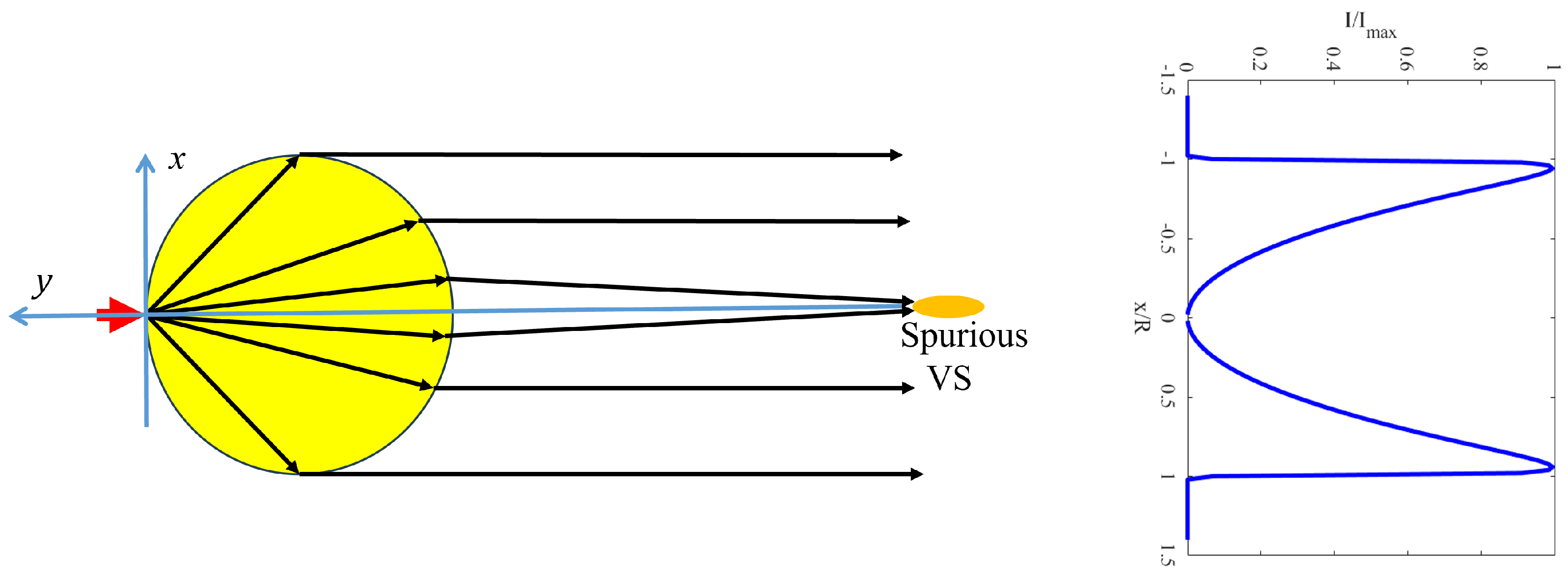
We numerically found that the approximate equivalence of two distances, Y and $y_{GO}$, does not hold when $n>1.4$. In this case, a GO is applied to an MP to find if Y gives no meaningful result. Paraxial rays cross out at a point located on the axis y behind the MP, forming a spurious VS (this VS is prohibited by the exact zero of the electromagnetic field on the axis y), whereas non-paraxial rays still diverge, and the crossings of their continuations give an extended VS in front of the MP.

If $n=1.44$, most of the rays transmitted through the MP are nearly parallel to the axis y, which implies $Y\to \infty$, whereas the paraxial rays deliver the spurious VS located at a large distance behind the MP. So, for $n>1.4$, the simplistic GO model becomes fully inadequate, and the Formula (3) is not applicable. The GO approximation applied to the rigorously simulated imaging beam at very large distances makes sense when $n>1.4$, but this method cannot be as straightforward as described above because the simulated imaging beam turns out to be collimated behind the MP and only starts to diverge at large distances from the MP.

In [95], the evolution of the imaging beam for microcylinders with $n>1.4$ was studied up to a distance of $\left|y\right|=3D_R$. These distances were insufficient to reliably evaluate the VS, but this study allowed us to reveal a novel scenario for MAN. This scenario is schematically presented in Figure 10. The previous imaging scheme (that illustrated by Figure 9) in our terminology corresponds to the conventional scenario of MAN. The ray picture for the transition case between the conventional and novel scenarios is presented in Figure 11.

If n lies in the range of 1.45–1.75 (we have not studied the case of higher n), the initially collimated imaging beam at a certain distance $\left|y\right|=D$ from the source (smaller than $D_R$ but comparable with it) sharply diverges. At distances of $\left|y\right|$∼$D_R$, its wavefront resembles a cylindrical wave. In the 3D case, it should be a spherical wave. So, the imaging beam of a dipole source located in front of our MP in this new scenario transmits through the MP as a set of parallel rays and, after a certain path, transforms into a diverging wave having the annular pattern with the exact zero on the beam axis. The phase center of this diverging wave is nothing but the novel VS, which is now located behind the MP at a substantial distance, $R<D<D_R$, from it. The coordinate of this point can also be denoted as $y_{GO}$ ($|y_{GO}|\equiv D$) because, treating this phase center as a point, we replace the diverging part of the imaging beam with a set of diverging rays, i.e., apply the same ray tracing approach as it was described above. For the ultimate spatial resolution, we have the following scenario: ${\delta }_{\min }=R{\delta }_V^{\min }/D$. Here, ${\delta }_V^{\min }$ is the minimal distance between the centers of two VSs when they are still resolvable.

In the simulations reported in [96], we studied the evolution of imaging beams until $1000\lambda$ and found ranges of n and $R/\lambda$, which offer both conventional and novel scenarios of MAN. The conventional scenario for microcylinders holds for n = 1.01–1.40 and $R/\lambda$ = 3–20. In these intervals, the simplistic approach (when the GO is applied to the MP treated as a usual lens) allows us to quite accurately find the axial location Y of the VS. For n = (1.41–1.44), the GO approximation does not work even when being applied to the rigorously simulated imaging beam. The reason is the interference of the transmitted rays with the rays corresponding to creeping waves bouncing off the MP. These waves, in case $1.41\le n\le 1.44)$, are present inside the area of the imaging beam, and the VS cannot arise in the wave beam impinging on the microscope objective.

The novel scenario of MAN holds when n = 1.45–1.75 and $R/\lambda$ = 3–20. For the most values of parameters lying in these intervals, the GO approximation applied to the diverging beam is suitable to find $y_{GO}$. When $R/\lambda$ = 4–6 and n = (1.45–1.75), the distance of the VS from the center of the MP is maximal and is rather close to $D_R$. Since $M=(D-R)/R$, we have $M\approx D_R/R=2R/\lambda$. In accordance with this estimate, in the novel scenario, the magnification may attain 12, even for a cylinder. If $n>1.44$ and $R/\lambda >6$, the distance D gradually decreases versus $R/\lambda$. Therefore, for larger R, the predicted magnification is also equal to 10–12. Recall that the known experiments with glass microcylinders operating in the conventional regime M = 2–3. Therefore, the novel regime promises nearly five-fold improvement. A glass microsphere offers magnification of M = 3–8 in the conventional non-resonant regime. Assume that the new scenario offers the same improvement as it grants for a microcylinder and microsphere. Then, we will obtain non-resonant magnification of M = 20–50 in this scenario. This amazing magnification may open new gates for biomedical investigations.

6.3. Bounds of Non-Resonant Ultimate Resolution for Microfibers

In the novel scenario, simulated in Figure 12, the imaging beam initially collimated after transmission through the MP sharply diverged at a distance of $|y_{G}O|=D\approx 13\lambda \approx 0.4D_R$ from the source and transformed into a nearly cylindrical wave. However, this method, as already noticed, does not allow us to find the transversal size of the VS. Therefore, in [96], we developed a method based on imaging beam inversion. Let us take the phase front S of the imaging beam at such a big distance that $\mathbf{E}$ on this surface would be practically tangential to it (the magnetic field vector $\mathbf{H}={\mathbf{z}}_0{H}_z$ is tangentially polarized in our 2D simulations everywhere). We may treat the electromagnetic field distribution simulated over S as the distribution of the Huygens sources. Using Green’s formula and neglecting the field outside the relevant area S, we may reconstruct the virtual past of the imaging beam in which there was neither a source nor an MP, but there was the wave beam incoming from $y\to \infty$. To calculate this virtual beam, we invert the magnetic field ($\mathbf{H}\to -\mathbf{H}$), keeping the same $\mathbf{E}$ on S, and calculate the inverted (backward) beam in free space.

Since the phase front S is not ideally circular and $\mathbf{E}$ is not ideally tangential to it, our inverted beam does not converge into a point. It forms a waist of effective width $d_V$ in a certain plane $y=y_W$, where its phase front becomes flat. Behind this plane, the backward beam diverges again and travels towards $y\to \infty$. Indeed, the zero field remains at the center of the waist point $(y=y_W,x=0)$. If we now invert the magnetic field $\mathbf{H}$ of the backward beam in this waist plane and apply Green’s formula once more, we will obtain exactly the same imaging beam created by the dipole source and the glass MP.

The waist of the inverted beam can be interpreted as the VS because only in the plane $y=y_W$ the wavefront of this beam is flat, and two halves of the piece $d_V$ may be treated as two opposite-phase finite-size Huygens elements. The electric dipole moments of these Huygens’ sources are oriented along x and are proportional to $H(x=d_V/2,y=y_W)d_V$ and the magnetic dipole moments are proportional to $E(x=d_V/2,y=y_W)d_V$ and are oriented along z. This anti-symmetric pair of Huygens’ elements creates nearly the same imaging beam as that created by our radial dipole and the glass MP. So, this pair of finite-size Huygens’ elements is our VS.

This approach works very well if the wavefront S is selected so that $\mathbf{E}$ is really tangential to it. In Figure 12, all wavefronts corresponding to $\left|y\right|>7D_R$ are suitable for simulating the backward beam, and a further increase of the distance does not reduce the width $d_V$ of the virtual source. Indeed, the field distribution in the backward beam is qualitatively different from that in the imaging beam propagating forward. It is not surprising that the Green formula demands the integration of the Huygens sources over a closed surface, whereas, when calculating the backward beam, we skip the area located beside the imaging beam. However, in MAN, if the objective lens develops, namely the imaging beam, the side-lobes completely spread and form a uniform background before they attain the microscope. Our method allows us to determine the VS that is maximally close to that seen with the microscope.

Indeed, this method is applicable to both conventional and novel scenarios. In the conventional scenario (when $n<1.4$ and the VS is formed in front of the MP), this method and the method based on the GO mutually validate one another because we numerically obtained $y_W\approx y_{GO}$. Moreover, if the radius of the MP is sufficiently large, $y_{GO}\approx Y$ and $y_W\approx Y$. In other words, the VS estimated treating the MP as a spherical lens nearly coincides with that obtained by our full-wave method for sufficiently large MPs. In Figure 13, we present an illustrative example of such simulations. Here, the phase front of the imaging beam becomes nearly circular when $\left|y\right|$ exceeds $D_R$. We have chosen the line S in the region when $\left|y\right|\approx 2D_R$. In this case, the backward beam has the waist $y_W$ in front of the MP and $y_W\approx y_{GO}\approx Y$.

Now, let us estimate the ultimate lateral resolution, which corresponds to the given magnification M. Unfortunately, the method of calculating it via the distribution of the light intensity in the imaging beam created by the VS at macroscopic distances (like it was done in [84,86]) cannot be applied. This method is elaborated for wave beams of the Gaussian type, i.e., those having the maximum intensity on the beam axis. However, our imaging beam is annular. Therefore, in our studies, we only evaluated the pessimistic and optimistic bounds of the ultimate resolution and compared them to the known experimental values for the glass microfiber. We saw that these values always lie in between these extremities.

In accordance with the Rayleigh criterion, two wave beams are resolved if the distance between their axes equals their effective widths defined at the level of 70% to the maximum. However, this criterion was elaborated only for the case when the intensity distributions of two beams are taken in the same plane. Since we cannot calculate the point-spread function in the microscope image plane, we have to resolve two VSs corresponding to two imaging beams with non-parallel axes. Respectively, the two VSs are defined in two different planes. Their mutual overlapping may not be so important for the resolution simply because they produce two wave beams which diverge from one another on the path towards the microscope. However, for a pessimistic estimate of the ultimate resolution, we may neglect this divergence. In this estimation, two VSs are assumed to be created in the same plane. Then, they are distinguished if their cross-sections overlap not critically, i.e., so that the null of one beam is not yet veiled by the maximum of another one. The analysis of the intensity distribution in the waist of the backward beam shows that this pessimistic ultimate resolution (that we denote below ${\delta }_{\min }^{\prime }$) corresponds to the case when ${\delta }_V\approx 2d_V/\pi$. Then, we have ${\delta }_{\min }^{\prime }=2d_V/\pi M$.

In the optimistic estimation, we neglect the finite size of the VS. As already discussed, in this estimation, two VSs are resolved if the distance ${\delta }_V$ between them is equal to $\lambda /2$ or larger. Therefore, the optimistic estimate for the ultimate resolution is ${\delta }_{\min }^{\prime \prime }=\lambda /2M$. The bounds of ultimate resolution for four sets of parameters of a microcylinder are given in

Table 1. Pessimistic and optimistic estimates of the resolution for two scenarios.

	Conventional Sc. ($\mathit{n}=1.3$)		Novel Sc. ($\mathit{n}=1.6$)
R	${\delta }_{\min }^{\prime }$	${\delta }_{\min }^{″}$	${\delta }_{\min }^{\prime }$	${\delta }_{\min }^{″}$
4.3$\lambda$	0.72$\lambda$	0.18$\lambda$	0.38$\lambda$	0.04$\lambda$
10.45$\lambda$	0.97$\lambda$	0.39$\lambda$	0.54$\lambda$	0.05$\lambda$

. Size parameters and refraction indices for this table were chosen to enable both scenarios of super-resolution and to avoid the resonances of the MP.

Experimental data for the ultimate resolution granted by glass microfibers are known only for a conventional scenario, which is implemented with the help of the liquid host medium. For example, in [22], the super-resolution ${\delta }_{\min }\approx 0.2\lambda$ was granted by a microfiber of silica ($n_s=1.47$) with a radius of $R\approx 7\lambda$ submerged into a drop of acetone into which the objective lens was also submerged. In the acetone, the relative index of silica reduces to $n\approx 1.1$, and the experimental result of [22] turns out to be close to the lower bound of the interval $[{\delta }_{\min }^{\prime }=0.83\lambda ,{\delta }_{\min }^{\prime \prime }=0.19\lambda ]$ that we obtained for $n=1.1$ and $R=7\lambda$. In our theory, much better resolution arises without acetone in the novel scenario, but the authors of [22] tuned their microscope only for the conventional scenario when the VS is located below the real source.

Treating the value in the middle of the interval $[{\delta }_{\min }^{\prime \prime },{\delta }_{\min }^{\prime }]$ as the true ultimate resolution, we revealed an important feature of the novel scenario of MAN. When the radius of the MP increases starting from the optimal value $R\approx 4\lambda$, the ultimate resolution worsens gradually. In the case $n=1.6$, it achieves $\lambda /2$ when $R\approx 20\lambda$. Meanwhile, when R is decreased compared to R = (3–4)$\lambda$ (the exact value depends on n), the spatial resolution worsens sharply. The possible reason for this difference will be discussed below.

6.4. Mechanism of the Object Radial Polarization

Now, let us consider the origin of the radial (with respect to the MP) polarization of an object in the case when it is illuminated by a normal incidence plane wave like in [20]. If the object area is illuminated by daylight or the obliquely incident laser light, the radial component of the electric field has the same order of magnitude as the tangential component. Due to the strong diffraction spread, the imaging beam produced by the tangential polarization represents a parasitic luminescent background, which should not veil the subwavelength image created by the radial polarization.

However, if the object is illuminated by a normal incident light, as shown in Figure 14, the incident electric field is horizontal, and its radial component is very small. In MAN, the area in which super-resolution is achieved represents a circle of micron radius centered by the touch point of a sphere (for a cylinder, it is a strip whose width is equal to 2–3 $\mathsf{\mu }$m). If the radial polarization is very small, the subwavelength image will be veiled by the parasitic spread image created by the tangential polarization.

Let us qualitatively consider two nanoscatterers located in the crevice beneath the MP, as shown in Figure 14. Let a nanoscatterer located in the left part of the crevice and characterized by the central angle $\alpha \le 0.3$ rad be closer to the MP rest point $x=0$ than the other one located in the right part of the crevice and characterized by the central angle ${\alpha }^{\prime }>0.5$ rad. Let both nanoscatterers be illuminated by the laser light normally incident on the substrate interface from the bottom. Our simulations have shown that for nanoscatterers located at $\alpha \le 0.3$ rad, a strong cross-polarization effect arises, and for $\alpha \ge 0.5$, this effect is absent.

Without the cross-polarization effect, the radial component of the dipole moment of the left scatterer would be equal to $p_{rg}\approx p\alpha \ll p$, where p is the absolute value of its dipole moment and $p_{rg}$ is the “geometric” radial component corresponding to the horizontal orientation of the dipole $\mathbf{p}$. Due to the cross-polarization effect, the radial dipole moment $p_r$ turns out to be much larger than $p_{rg}$. For $R=7\lambda$ and $n>1.5$, the corresponding area may be determined as $\left|x\right|<2\lambda =1.1$ mm. For $R=4\lambda$ and $n>1.5$ mm, the area of strong cross-polarization was determined as $\left|x\right|<1.5\lambda$. Below, we call the region of such strong cross-polarization the object area.

For the right nanoscatterer in Figure 14, which is located beyond the object area, the impact of the crevice shape is not important, and its dipole moment ${\mathbf{p}}^{\prime }$ remains practically horizontal. The radial polarization of this nanoscatteter is purely geometric $p_r^{\prime }=p_{rg}^{\prime }$, i.e., for angles ${\alpha }^{\prime }\ll 1$, we have $p_r^{\prime }\ll p^{\prime }$. For larger angles, $p_r^{\prime }$ approaches $p^{\prime }$, but the distance from the nanoscatterer to the MP becomes large, and the near-field coupling disappears. This is the reason why super-resolution cannot be achieved beyond a narrow object area.

Numerical simulations reported in [97] revealed that the cross-polarization of nanoscatterers located in the object area arises mainly due to two physical effects. The first effect is the near-field coupling of the nanoscatterer and the MP. In the zero approximation, the radial polarization of the nanoscatterer is equal to $p_{rg}$, which is nonzero everywhere besides the MP rest point. This small radial dipole creates the radially polarized near field. Though a dipole does not radiate along its axis, its near field is maximal, namely in the axial direction. Therefore, a small part of the MP located in front of the radial dipole turns out to be radially polarized. The interaction of two collinear dipoles across the nanogap amplifies both these dipole moments compared to their values taken in the zero approximation. This effect is basically the same on which the metal-enhanced fluorescence is based (see, e.g., [100]). In nanophotonics, this effect results in the so-called photon tunneling, i.e., the enhanced transmission of evanescent waves polarized normally to the dielectric-vacuum interfaces across the vacuum nanogap between two dielectric media. It is the key physical effect on which the operation of the so-called near-field thermophotovoltaic systems is based [101]. The second effect, also resulting in cross-polarization, may either enhance radial polarization or completely suppress it. This is the effect of the MP touch point, which reflects the electric field created by the nanoscatterer back to the crevice.

In Figure 15a, we show the simulated structure in which the nanoscatterer is a silver nanocylinder of diameter 10 nm located in the object area (marked by red) on the silicon substrate. The coordinate x of its center is counted from the touch point of the microparticle. Figure 15b depicts the results for $p_r/p$ as a function of $x/\lambda$ for $R=7\lambda$ and four different values of n. The interplay of the photon tunneling and the reflection from the touch point results in the spatial oscillations of the radial polarization. If n = 1.6–1.7, the cross-component of the electric field attains the maximum at $\left|x\right|$ = (0.1–0.2)$\lambda$, where the 30-fold enhancement of $p_r$ compared to $p_{rg}$ is achieved. For n = 1.4–1.5, there is a deep minimum in the region x = (0.7–0.8)$\lambda$. Thus, for MPs with small indices, the cross-polarization effect may be destructive for the radial polarization (in a part of the object area). If $n>1.5$, the constructive effect for the cross-polarization prevails in the whole object area ($\left|x\right|<1.5\lambda$). This result was confirmed by a set of simulations into which the substrates of different thicknesses and refractive indices were studied.

Simulations of [97] have shown that the significant radial component of the object polarization in MAN arises in most parts of the object area, even in the case when the object is illuminated normally by coherent light. The simulations were carried out for microcylinders but the physics, indeed, remains the same for microspheres. So, we have completed the quantitative explanation of MAN and may start the general discussion.

7. Discussion of Our Theoretical Results

The initial experiments reported in the seminal paper [20] have shown that the GO correctly describes the formation of a magnified virtual object by a dielectric microsphere with modest values of the refractive index. Namely, the location of virtual sources forming the virtual object was adequately predicted when the microsphere was treated as a usual macroscopic spherical lens. In this work, the unexpected predictive power of the GO was not explained, and in further works on MAN, it was treated as an occasional coincidence because the GO should not have worked for spheres whose radius was comparable with $\lambda$ especially if the distance d between the object and the sphere was much smaller than $\lambda$.

The author of the present paper assumed that it was not a coincidence but resulted from two factors. Th first factor is the critical suppression of the diffraction in the wave beam transmitted through a glass microsphere or a microcylinder. The second factor is the photon tunneling, which effectively unites the luminescent object and the microparticle. Both these effects demand the radial (with respect to the MP) polarization of the object. For a tangentially polarized dipole source, nothing restricts the diffraction spread of the wave beam transmitted though the sphere, and the photon tunneling is weaker. After publishing this guess in [31], the analytical study [93] was found whose main message was namely, the unexpected predictive power of the GO for the wave beam created by a radially polarized dipole behind a dielectric sphere whose radius was larger than $\lambda$ but comparable with it. Since the photon tunneling was already well studied, the only question left to explain MAN was as follows: is the reduction in the diffraction in the case of the normally polarized source sufficient for super-resolution?

So, to answer this question, the group of the author in 2020–2022 performed extensive numerical simulations using the COMSOL Multiphysics software and a supercomputer. We simulated and thoroughly analyzed the evolution of the 2D imaging wave beam for both tangentially and radially polarized dipole line sources in the case of the glass microparticle being a microcylinder. In general, these studies confirmed the author’s hypothesis. Let us now discuss the important details of MAN we have revealed.

If the refractive index of the MP is small ($n<1.4$), the GO can be applied in a simplistic way, treating the MP as a cylindrical lens. As well, in papers about spherical MAN where the same approach is successful when $n<1.5$, this approach allows one to predict the location of the virtual source corresponding to a point dipole line in a broad range $R/\lambda$ = 3–20. The diffraction effects are responsible for the effective size of this VS but do not change the estimate of its location.

In the case of a tangential dipole, the size of the VS resulting from the diffraction and estimated through the deviations of the wave fronts in the imaging beam from the concentric circles is much larger than $\lambda$. It does not offer the super-resolution in spite of the magnification granted by the glass MP. However, if the dipole located near its surface is polarized radially, the size of the virtual source turns out to be of the order of $\lambda$. Together with the magnification M = 3–4, this size enables the super-resolution in the case $n<1.4$ and R = (3–20)$\lambda$.

However, in the most interesting case, when $n>1.4$, the treatment of a glass microcylinder as a usual lens becomes meaningless. For n = 1.40–1.44, the super-resolution is not possible for any size parameters of the microcylinder due to the interference pattern caused by the ejection of creeping waves into the paraxial region. If n = 1.45–1.75, the super-resolution again becomes possible for glass microcylinders with R = (3–20)$\lambda$. In this case, the VS is formed not in front of the MP but at a large distance D behind it, which is still smaller than the Rayleigh range $D_R$ but comparable with it. The imaging beam corresponding to a dipole source located on the surface of the MP keeps collimated until this distance and then sharply diverges. This diverging beam has a spread phase center that represents the VS in this novel scenario of MAN, existing up to now only in our theory. Indeed, the effective size of this VS is much larger than $\lambda$; it is of the order of R, but the distance D is much larger, and the super-resolution in our calculations is maximal, namely in this new scenario. To estimate this size, we have elaborated a new method which allowed us to obtain the pessimistic and optimistic bounds for the size of the VS. If we identify the middle of this interval with the true size of the VS, the novel scenario of MAN grants a magnification which is 4–5 times higher than that in the conventional scenario and may attain $M=20$.

An important physical mechanism that enables MAN when the illumination of the object is normal to the substrate surface is the constructive cross-polarization of the object. It results in a drastic increase in the radial (with respect to the MP) polarization of the object. The main underlying physics of the effect is photon tunneling.

Now, let us discuss two important issues: (1) the intervals of size parameters and refractive indices suitable for MAN and (2) the possibility of MAN for distant objects.

When $R/\lambda <3$, the rays inside the MP are not formed, and the GO cannot describe the imaging beam for any n. There is no magnification for a set of dipole sources composing the object. Indeed, without a magnification, two radial dipoles cannot be resolved if the gap $\delta$ between them is deeply subwavelength because in the imaging beam, the zero of one dipole pattern is veiled by the nonzero radiation of another dipole in the same direction. This is why, for the super-resolution, there is a short-wave threshold of the size parameter $R/\lambda$. For example, $n=1.6$ and $R/\lambda =3$ in our simulations correspond to the absence of magnification and super-resolution, whereas $n=1.6$ and $R/\lambda =3.5$ correspond to the magnification $M\approx 20$ and resolution $({\delta }_{\min }^{\prime }+{\delta }_{\max }^{\prime })/2\approx 0.19\lambda$.

The size parameter $R/\lambda$ grows compared to this optimal value at which the super-resolution would sharply disappear. The resolution worsens gradually versus $R/\lambda$ and exceeds $\lambda /2$ within the interval $R/\lambda$ = 8–20 (the corresponding value of the size parameter depends on n).

Now, let us discuss the imaging of the objects substantially distant from the MP. Indeed, a formula similar to (3) can be easily derived for nonzero distances d from the dipole to the MP. However, if $d<\lambda /5$, this formula is not needed. In this case, the photon tunneling tightly couples the radial dipole to the microparticle, and the imaging beam is formed in the same way as if the dipole was located exactly on the surface of the glass.

When d∼$\lambda$, it is not so. Experiments in [22] showed that the MPs separated from the objects by a micron layer of a lubricant do not grant the super-resolution. The most probable reason for this is that $\lambda$ is comparable with R, though smaller. Applying the simplistic GO approach to the case when d is comparable with R, we obtain two VSs: one corresponding to paraxial rays, which is located in front of the microparticles, and the other one is either inside it or behind it, depending on n. This ambiguity means that the GO approach does not work. In this situation, the suppression of the diffraction on the imaging beam axis is hardly helpful for the resolution. It means that the conventional scenario of MAN for substantially distant objects is not possible. As to the novel scenario, this question is open. In our simulations, we have not really studied the case when $d\sim \lambda$ because the first simulation has shown that in this case, the cross-polarization effect (necessary in the case when the illumination is normal to the substrate) is practically absent. However, the illumination may be oblique, and the object may be polarized radially even when substantially distanced from the MP. This case needs further investigation.

8. Conclusions and Outlook

In this overview paper, we familiarized ourselves with the microparticle-assisted nanoscopy considered in the context of the linear methods of direct subwavelength imaging. To understand the uniqueness of this method we considered all other LFSI methods: indirect and direct ones. We discussed and demystified the popular myth that the Abbe diffraction limit is fundamental and may be beaten in direct far-field imaging only with the help of metamaterials, evanescent waves, and their conversion.

We considered the main experimental achievements of MAN and reviewed the state-of-the-art in its theoretical investigations. We have seen that beyond the resonances of MP or elements on its substrate, the super-resolution results are not from wave conversion and have nothing to do with the phenomenon of the photonic nanojet. It is enabled by partial suppression of diffraction which makes the description of the imaging in terms of the GO possible. This suppression of diffraction occurs if and only if the object has sufficient radial polarization with respect to the MP. This claim was confirmed by the analysis of a huge amount of numerical data.

In these simulations, we revealed not only the diffraction suppression for the radial polarization of the object but also a novel scenario of MAN, which holds in the case of large values of the refractive index. We developed a method which allowed us to calculate the virtual source corresponding to a real dipole source. Using this method, we obtained optimistic and pessimistic estimates for the ultimate resolution in both scenarios of MAN. Also, with this method, we validated the application of the GO for the case of small refractive indices of the MP. Including the substrate in our simulations, we have obtained an explanation of why the radial polarization of the object is not weaker than that of the tangential one, even when the object is illuminated by the normally incident plane wave.

So, the origin of MAN and the operation of MPs in the non-resonant MAN are explained. MAN is the manifestation of the fact that the Abbe limit (0.5–0.6)$\lambda$ is not something fundamental. It can be beaten without conversion of evanescent/surface waves to propagating ones simply due to the advantageous polarization of the object and lensing properties of the MP. Like in the far-field SPRM and in the hyperlens microscopy, in the MAN, the impact of the magnification dominates over the impact of the additional diffraction.

As to the outlook of MAN, one may suggest the following action points:

• Experimental confirmation of the novel scenario. For it, one should start by studying the 2D MAN, e.g., the case of a microfiber, because for this case, the needed parameters have been calculated. The microscope should be tuned in accordance with the predicted location of the virtual object, i.e., in the region over the microparticle and not in the substrate as in the conventional scenario. If our theory promising huge magnification (up to 20) is confirmed, it will open a new chapter in MAN.
• A numerical and experimental study of MAN in the case when the radially polarized object is located at a substantial distance d from the strongly refracting microparticle. In the experiment, one may use a weakly refractive layer of variable thickness. For example, an MP with high n may be incorporated into a low-n polymer film, and the distance d between the bottom edge of the MP and the bottom surface of the polymer may be gradually reduced by chemical etching. Since the radial polarization of the normally illuminated object does not arise when d is substantial, the illumination should be oblique. Again, this study will open a new chapter in MAN.
• Creation of a technique which would allow one to drag an array of the MPs over a macroscopic area of a substrate covered by the objects. Friction and Van der Waals forces may be compensated by specially engineered repulsive forces (e.g., electrostatic forces between the film comprising the MPs and the substrate).

There is no doubt that the successful completion of these three studies will have a revolutionary impact on the whole of subwavelength imaging.

References

1. Abbe, E. Beiträge zur Theorie des Mikroskops und der mikroskopischen Wahrnehmung. Arch. Mikrosk. Anat. 1873, 9, 413–468. [Google Scholar] [CrossRef]
2. Airy, G. On the Diffraction of an Object-Glass with Circular Aperture. Trans. Camb. Philos. Soc. 1835, 5, 283–291. [Google Scholar]
3. Rayleigh, L.F. Investigations in optics, with special reference to the spectroscope. Lond. Edinb. Dublin Philos. Mag. J. Sci. 1879, 8, 261–274. [Google Scholar] [CrossRef]
4. Born, M.; Wolf, E. Principles of Optics; Pergamon Press: Oxford, UK, 1965. [Google Scholar]
5. Liang, C.; Wu, G.; Wang, F.; Li, W.; Cai, Y.; Ponomarenko, S.A. Overcoming the classical Rayleigh diffraction limit by controlling two-point correlations of partially coherent light sources. Opt. Express 2017, 25, 135–214. [Google Scholar] [CrossRef]
6. Rueckner, W.; Papaliolios, C. How to beat the Rayleigh resolution limit: A lecture demonstration. Am. J. Phys. 2002, 70, 587–594. [Google Scholar] [CrossRef]
7. Paur, M.; Stoklasa, B.; Hradil, Z.; Sanchez-Soto, L.L.; Rehacek, J. Achieving the ultimate optical resolution. Optica 2016, 3, 1144–1147. [Google Scholar] [CrossRef]
8. Lipson, S.G.; Lipson, H.; Tannhauser, D.S. Optical Physics; Cambridge University Press: Cambridge, MA, USA, 1995; pp. 345–354. [Google Scholar]
9. Ash, E.A.; Nicholls, G. Super-resolution aperture scanning microscope. Nature 1972, 237, 510–512. [Google Scholar] [CrossRef]
10. Dürig, U.; Pohl, D.W.; Rohner, F. Near-field optical-scanning microscopy. J. Appl. Phys. 1986, 59, 3318–3327. [Google Scholar] [CrossRef]
11. Pendry, J.B. Negative refraction makes perfect lens. Phys. Rev. Lett. 2000, 85, 3966–3969. [Google Scholar] [CrossRef]
12. Veselago, V.G. The electrodynamics of substances with simultaneously negative values of epsilon and mu. Sov. Phys. Uspekhi 1968, 10, 509–514. [Google Scholar] [CrossRef]
13. Baryshnikova, K.V.; Kharintsev, S.S.; Belov, P.A.; Ustimenko, N.A.; Tretyakov, S.A.; Simovski, C.R. Metalenses for subwavelength imaging. Phys. Uspekhi 2022, 65, 355–378. [Google Scholar] [CrossRef]
14. Rho, J.; Ye, Z.; Xiong, Y.; Yin, X.; Liu, Z.; Choi, H.; Bartal, G.; Zhang, X. Spherical hyperlens for two-dimensional sub-diffractional imaging at visible frequencies. Nat. Commun. 2010, 1, 143. [Google Scholar] [CrossRef]
15. Lu, D.; Liu, Z. Hyperlenses and metalenses for far-field super-resolution imaging. Nat. Commun. 2012, 3, 1205. [Google Scholar] [CrossRef] [PubMed]
16. Hayashi, J.G.; Stefani, A.; Antipov, S.; Lwin, R.; Jackson, S.D.; Hudson, D.D.; Fleming, S.; Argyros, A.; Kuhlmey, B.T. Towards subdiffraction imaging with wire array metamaterial hyperlenses at MIR frequencies. Opt. Express 2019, 27, 21420–21434. [Google Scholar] [CrossRef] [PubMed]
17. Zhu, H.; Yan, B.; Zhou, S.; Wang, Z.; Wu, L. Synthesis and super-resolution imaging performance of a refractive-index-controllable microsphere superlens. J. Mater. Chem. C 2015, 3, 10907–10915. [Google Scholar] [CrossRef]
18. Hell, S.; Wichmann, J. Breaking the diffraction resolution limit by stimulated emission: Stimulated-emission-depletion fluorescence microscopy. Opt. Lett. 1994, 19, 780–782. [Google Scholar] [CrossRef]
19. Astratov, V.N.; Sahel, Y.B.; Eldar, Y.C.; Huang, L.; Ozcan, A.; Zheludev, N.; Zhao, J.; Burns, Z.; Liu, Z.; Narimanov, E.; et al. Roadmap on Label-Free Super-Resolution Imaging. Laser Photonic Rev. 2023, 17, 2200029. [Google Scholar] [CrossRef]
20. Wang, Z.; Guo, W.; Li, L.; Lukyanchuk, B.; Khan, A.; Liu, Z.; Chen, Z.; Hong, M. Optical virtual imaging at 50 nm lateral resolution with a white-light nanoscope. Nat. Commun. 2011, 2, 218. [Google Scholar] [CrossRef]
21. Allen, K.; Farahi, N.; Li, Y.; Limberopoulos, N.; Walker, D.; Urbas, A.; Astratov, V.N. Overcoming the diffraction limit of imaging nanoplasmonic arrays by microspheres and microfibers. Opt. Express 2015, 23, 24484–24496. [Google Scholar] [CrossRef]
22. Allen, K.W.; Farahi, N.; Li, Y.; Limberopoulos, N.I.; Walker, D.E., Jr.; Urbas, A.M.; Liberman, V.; Astratov, V.N. Super-resolution microscopy by movable thin-films with embedded microspheres: Resolution analysis. Ann. Phys. 2015, 527, 513–522. [Google Scholar] [CrossRef]
23. Darafsheh, A. Microsphere-assisted microscopy. J. Appl. Phys. 2022, 27, 031102. [Google Scholar] [CrossRef]
24. Yang, H.; Moullan, N.; Auwerx, J.; Gijs, M.A. Super-resolution biological microscopy using virtual imaging by a microsphere nanoscope. Small 2014, 10, 1712–1718. [Google Scholar] [CrossRef] [PubMed]
25. Upputuri, P.K.; Pramanik, M. Microsphere-aided optical microscopy and its applications for super-resolution imaging. Opt. Commun. 2017, 404, 32–41. [Google Scholar] [CrossRef]
26. Li, L.; Guo, W.; Yan, Y.; Lee, S.; Wang, T. Label-free super-resolution imaging of adenoviruses by submerged microsphere optical nanoscopy. Light Sci. Appl. 2013, 2, e104. [Google Scholar] [CrossRef]
27. Lecler, S.; Perrin, S.; Leong-Hoi, A.; Montgomery, P. Photonic jet lens. Sci. Rep. 2019, 9, 4725. [Google Scholar] [CrossRef]
28. Cao, Y.; Yang, S.; Wang, D.; Wang, J.; Ye, Y.H. Surface plasmon-enhanced dark-field microsphere-assisted microscopy. Opt. Express 2023, 31, 8641–8649. [Google Scholar] [CrossRef]
29. Huszka, G.; Gijs, M. Super-resolution optical imaging: A comparison. Micro Nano Eng. 2019, 2, 7–28. [Google Scholar] [CrossRef]
30. Kassamakov, I.; Lecler, S.; Nolvi, A.; Leong-Hoï, A.; Montgomery, P.; Haeggström, E. 3D Super-Resolution Optical Profiling Using Microsphere Enhanced Mirau Interferometry. Sci. Rep. 2017, 7, 3683. [Google Scholar] [CrossRef]
31. Heydarian, R.; Simovski, C.R. The role of normal polarization in far-field subwavelength imaging by a dielectric microsphere or microcylinder. J. Opt. 2020, 22, 075002. [Google Scholar] [CrossRef]
32. Siedentopf, H.; Zsigmondy, R.E. Über Sichtbarmachung und Grössenbestimmung ultramikroskopischer Teilchen, mit besonderer Anwendung auf Goldrubingläser. Ann. Phys. 1903, 10, 1–39. [Google Scholar]
33. Lewis, A.; Isaacson, M.; Harootunian, A.; Muray, A. Development of a 500 Angström spatial resolution light microscope. Ultramicroscopy 1984, 13, 227–231. [Google Scholar] [CrossRef]
34. Lukosz, W. Optical Systems with Resolving Powers Exceeding the Classical Limit. J. Opt. Soc. Am. 1966, 56, 1463–1472. [Google Scholar] [CrossRef]
35. Cox, I.; Sheppard, C.J.R. Information capacity and resolution in an optical system. J. Opt. Soc. Am. 1986, 3, 1152–1158. [Google Scholar] [CrossRef]
36. Liu, Z.; Durant, S.; Lee, H.; Pikus, Y.; Fang, N.; Xiong, Y.; Sun, C.; Zhang, X. Far-Field Optical Superlens. Nano Lett. 2007, 7, 403–408. [Google Scholar] [CrossRef] [PubMed]
37. Rumelhart, D.E.; Hinton, G.E.; Williams, R.J. Learning representations by back-propagating errors. Nature 1986, 323, 533–536. [Google Scholar] [CrossRef]
38. Candes, E.; Romber, J. Sparsity and incoherence in compressive sampling. Inverse Probl. 2007, 23, 969. [Google Scholar] [CrossRef]
39. Szameit, A.; Shechtman, Y.; Osherovich, E.; Bullkich, E.; Sidorenko, P.; Dana, H.; Steiner, S.; Kley, E.B.; Gazit, S.; Cohen-Hyams, T.; et al. Sparsity-based single-shot subwavelength coherent diffractive imaging. Nat. Mater. 2012, 11, 455–459. [Google Scholar] [CrossRef]
40. Gazit, S.; Szameit, A.; Eldar, Y.C.; Segev, M. Super-resolution and reconstruction of sparse sub-wavelength images. Opt. Express 2009, 17, 23920–23946. [Google Scholar] [CrossRef]
41. Zhang, T.; Godavarthi, C.; Chaumet, P.C.; Maire, G.; Giovannini, H.; Talneau, A.; Allain, M.; Belkebir, K.; Sentenac, A. Far-field diffraction microscopy at lambda/10 resolution. Optica 2016, 3, 609–612. [Google Scholar] [CrossRef]
42. Pillarik, M.; Sandohdar, V. Direct optical sensing of single unlabelled proteins and super-resolution imaging of their binding sites. Nat. Commun. 2014, 5, 4495. [Google Scholar] [CrossRef]
43. Taylor, R.W.; Sandohdar, V. Interferometric Scattering Microscopy: Seeing Single Nanoparticles and Molecules via Rayleigh Scattering. Nano Lett. 2019, 19, 4827–4835. [Google Scholar] [CrossRef] [PubMed]
44. Pu, T.; Ou, J.Y.; Savinov, V.; Yuan, G.; Papasimakis, N.; Zheludev, N.I. Unlabeled Far-Field Deeply Subwavelength Topological Microscopy (DSTM). Adv. Sci. 2021, 8, 2002886. [Google Scholar] [CrossRef] [PubMed]
45. Huang, F.M.; Zheludev, N.I. Super-resolution without evanescent waves. Nano Lett. 2009, 9, 1249–1254. [Google Scholar] [CrossRef] [PubMed]
46. Gustafsson, M.G. Surpassing the lateral resolution limit by a factor of two using structured illumination microscopy. J. Microsc. 2000, 192, 82–87. [Google Scholar] [CrossRef] [PubMed]
47. Zernike, F. How I Discovered Phase Contrast. Science 1955, 121, 345–349. [Google Scholar] [CrossRef]
48. Kemmler, M.; Fratz, M.; Giel, D.; Saum, N.; Brandenburg, A.; Hoffmann, C. Noninvasive time-dependent cytometry monitoring by digital holography. J. Biomed. Opt. 2007, 12, 064002. [Google Scholar] [CrossRef]
49. Fukutake, N. A general theory of far-field optical microscopy image formation and resolution limit using double-sided Feynman diagrams. Sci. Rep. 2020, 10, 17644. [Google Scholar] [CrossRef]
50. Shemonski, N.D.; South, F.A.; Liu, Y.Z.; Adie, S.G.; Carney, P.S.; Boppar, S.A. Computational high-resolution optical imaging of the living human retina. Nat. Photonics 2015, 9, 440–443. [Google Scholar] [CrossRef]
51. Mico, V.; Zheng, J.; Garcia, J.; Zalevsky, Z.; Gao, P. Resolution enhancement in quantitative phase microscopy. Adv. Opt. Photonics 2019, 11, 135–214. [Google Scholar] [CrossRef]
52. Toraldo di Francia, G. Super-gain antennas and optical resolving power. Nuovo Cimento Suppl. 1952, 31X, 426–438. [Google Scholar] [CrossRef]
53. Narimanov, E. Resolution limit of label-free far-field microscopy. Adv. Photonics 2019, 1, 056003. [Google Scholar] [CrossRef]
54. Lee, Y.U.; Zhao, J.; Ma, Q.; Khorashad, L.K.; Posner, C.; Li, G.; Wisna, G.B.M.; Burns, Z.; Zhang, J.; Liu, Z. Metamaterial assisted illumination nanoscopy via random super-resolution speckles. Nat. Commun. 2021, 12, 1559. [Google Scholar] [CrossRef] [PubMed]
55. Berry, M.V.; Popescu, S. Evolution of quantum superoscillations and optical superresolution without evanescent waves. J. Phys. A 2006, 39, 6965. [Google Scholar] [CrossRef]
56. Baskourelos, K.; Tsilipakos, O.; Stefański, T.; Galata, S.F.; Economou, E.N.; Kafesaki, M.; Tsakmakidis, K.L. Topological extraordinary optical transmission. Phys. Rev. Res. 2022, 4, L032011. [Google Scholar] [CrossRef]
57. Chernomyrdin, N.V.; Skorobogatiy, M.; Gavdush, A.A.; Musina, G.R.; Katyba, G.M.; Komandin, G.A.; Khorokhorov, A.M.; Spektor, I.E.; Tuchin, V.V.; Zaytsev, K.I. Quantitative super-resolution solid immersion microscopy via refractive index profile reconstruction. Optica 2021, 8, 1471–1480. [Google Scholar] [CrossRef]
58. Feynman, R.P.; Leighton, R.P.; Sands, M. The Feynman Lectures on Physics; Addison-Wesley: Reading, MA, USA, 2006; Chapter 30; Volume II. [Google Scholar]
59. Smolyaninov, I.I.; Elliott, J.; Zayats, A.V.; Davis, C.C. Far-Field Optical Microscopy with a Nanometer-Scale Resolution Based on the In-Plane Image Magnification by Surface Plasmon Polaritons. Phys. Rev. Lett. 2005, 94, 057401. [Google Scholar] [CrossRef]
60. Rothenhäusler, B.; Knoll, W. Surface–plasmon microscopy. Nature 1988, 332, 615–617. [Google Scholar] [CrossRef]
61. Kawata, S.; Inoue, Y.; Verma, P. Plasmonics for near-field nano-imaging and superlensing. Nat. Photonics 2009, 3, 388–394. [Google Scholar] [CrossRef]
62. Liu, Z. Plasmonics and Super-Resolution Imaging; Jenny Stanford Publishing: Stanford, CA, USA, 2017. [Google Scholar]
63. Jacob, Z.; Alekseyev, L.V.; Narimanov, E. Optical Hyperlens: Far-field imaging beyond the diffraction limit. Opt. Express 2006, 14, 8247. [Google Scholar] [CrossRef]
64. Salandrino, A.; Engheta, N. Far-field subdiffraction optical microscopy using metamaterial crystals: Theory and simulations. Phys. Rev. B 2006, 74, 075103. [Google Scholar] [CrossRef]
65. Smolyaninov, I.I.; Hung, Y.J.; Davis, C.C. Magnifying Superlens in the Visible Frequency Range. Science 2007, 315, 1699. [Google Scholar] [CrossRef] [PubMed]
66. Liu, Z.; Lee, H.; Xiong, Y.; Sun, C.; Zhang, X. Far-Field Optical Hyperlens Magnifying Sub-Diffraction-Limited Objects. Science 2007, 315, 1686. [Google Scholar] [CrossRef] [PubMed]
67. Zhang, X.; Adams, W.; Sadatgol, M.; Guney, D. Enhancing the resolution of hyperlens by the compensation of losses without gain media. Prog. Electromagn. Res. C 2016, 70, 1–7. [Google Scholar] [CrossRef]
68. Repän, T.; Lavrinenko, A.; Zhukovsky, S. Dark-field hyperlens: Super-resolution imaging of weakly scattering objects. Opt. Express 2015, 23, 25350–25364. [Google Scholar] [CrossRef]
69. Wang, W.; Yadav, N.; Shen, Z.; Cao, Y.; Liu, J.; Liu, X. Two-stage magnifying hyperlens structure based on metamaterials for super-resolution imaging. Optik 2018, 174, 199–206. [Google Scholar] [CrossRef]
70. Cang, H.; Salandrino, A.; Wang, Y.; Zhang, X. Adiabatic far-field sub-diffraction imaging. Nat. Commun. 2015, 6, 7942. [Google Scholar] [CrossRef]
71. Wang, J.; Jiang, R.; Yang, S.; Cao, Y.; Ye, Y.H. Microsphere-assisted dark-field microscopy based on a fully immersed low refractive index microsphere. Opt. Lett. 2023, 48, 1858–1861. [Google Scholar] [CrossRef]
72. Wang, F.; Liu, L.; Yu, H.; Wen, Y.; Yu, P.; Liu, Z.; Wang, Y.; Li, W.J. Scanning superlens microscopy for non-invasive large field-of-view visible light nanoscale imaging. Nat. Commun. 2016, 7, 13748. [Google Scholar] [CrossRef]
73. Huszka, G.; Gijs, M. Turning a normal microscope into a super-resolution instrument using a scanning microlens array. Sci. Rep. 2018, 7, 601. [Google Scholar] [CrossRef]
74. Maslov, A.V.; Astratov, V.N. Optical nanoscopy with contact Mie-particles: Resolution analysis. Appl. Phys. Lett. 2017, 110, 261107. [Google Scholar] [CrossRef]
75. Zhou, S.; Deng, Y.; Zhou, W.; Yu, M.; Urbach, H.P.; Wu, Y. Effects of whispering gallery mode in microsphere super-resolution imaging. Appl. Phys. B 2017, 123, 236. [Google Scholar] [CrossRef]
76. Bekirov, A.R.; Luk’yanchuk, B.; Wang, Z.; Fedyanin, A. Wave theory of virtual image. Opt. Mater. Express 2021, 11, 3646–3655. [Google Scholar] [CrossRef]
77. Yang, H.; Trouillon, R.; Huszka, G.; Gijs, M.A.M. Super-resolution Imaging of a Dielectric Microsphere Is Governed by the Waist of Its Photonic Nanojet. Nano Lett. 2016, 16, 4862–4870. [Google Scholar] [CrossRef] [PubMed]
78. Itagi, A.; Challener, W. Optics of photonic nanojets. J. Opt. Soc. Am. A 2005, 22, 2847–2858. [Google Scholar] [CrossRef]
79. Chen, Z.; Taflove, A.; Backman, V. Photonic nanojet enhancement of backscattering of light by nanoparticles: A potential novel visible-light ultramicroscopy technique. Opt. Express 2004, 12, 1214–1220. [Google Scholar] [CrossRef]
80. Heifetz, A.; Kong, S.C.; Sahakian, A.V.; Taflove, A.; Backman, V. Photonic nanojets. J. Comput. Theor. Nanosci. 2009, 6, 1979–1992. [Google Scholar] [CrossRef]
81. Kavungal, V.; Bo, L.; Wu, Q.; Teng, M. Study of whispering gallery modes in a cylindrical microresonator excited by a tilted fiber taper. In Proceedings of the 23rd International Conference on Optical Fibre Sensors, Santander, Spain, 2–6 June 2014; Volume 9157. [Google Scholar] [CrossRef]
82. Liu, C.Y.; Yeh, M.J. Experimental verification of twin photonic nanojets from a dielectric microcylinder. Opt. Lett. 2019, 44, 3262–3265. [Google Scholar] [CrossRef]
83. Li, H.; Song, W.; Zhao, Y.; Cao, Q.; Wen, A. Optical Trapping, Sensing, and Imaging by Photonic Nanojets. Photonics 2021, 8, 434. [Google Scholar] [CrossRef]
84. Maslov, A.; Astratov, V. Resolution and Reciprocity in Microspherical Nanoscopy: Point-Spread Function Versus Photonic Nanojets. Phys. Rev. Appl. 2019, 11, 064004. [Google Scholar] [CrossRef]
85. Osipov, A.V.; Tretyakov, S.A. Modern Electromagnetic Scattering Theory with Applications; John Wiley & Sons, Ltd.: New York, NY, USA, 2017. [Google Scholar] [CrossRef]
86. Yu, L.Y.; Cyue, Z.R.; Su, G.D.J. Three-stage full-wave simulation architecture for in-depth analysis of microspheres in microscopy. Opt. Express 2020, 28, 8862–8877. [Google Scholar] [CrossRef] [PubMed]
87. Glisson, A.; Wilton, D. Simple and Efficient Numerical Methods for Problems of Electromagnetic Radiation and Scattering from Surfaces. IEEE Trans. Antennas Propag. 1980, 28, 593–603. [Google Scholar] [CrossRef]
88. Rao, S.; Wilton, D.; Glisson, A. Electromagnetic Scattering by Surfaces of Arbitrary shape. IEEE Trans. Antennas Propag. 1982, 30, 409–417. [Google Scholar] [CrossRef]
89. Boudoukha, R.; Perrin, S.; Demagh, A.; Montgomery, P.; Demagh, N.E.; Lecler, S. Near-to-Far-Field Coupling of Evanescent Waves by Glass Microspheres. Photonics 2021, 8, 53. [Google Scholar] [CrossRef]
90. Minin, O.V.; Minin, I.V. Optical Phenomena in Mesoscale Dielectric Particles. Photonics 2021, 8, 591. [Google Scholar] [CrossRef]
91. Wang, H.; Zhang, J.; Wu, X.; Shen, D. On-resonance photonic nanojets for nanoparticle trapping. Opt. Express 2019, 27, 10472–10481. [Google Scholar] [CrossRef]
92. Sundaram, V.M.; Wena, S.B. Analysis of deep sub-micron resolution in microsphere based imaging. Appl. Phys. Lett. 2014, 105, 204102. [Google Scholar] [CrossRef]
93. Houdzoumis, V.A. Vertical electric dipole radiation over a sphere: Character of the waves that propagate through the sphere. J. Appl. Phys. 1999, 86, 3939–3942. [Google Scholar] [CrossRef]
94. Kravtsov, Y.A. Complex Rays and Complex Caustics. Radiophys. Quantum Electron. 1967, 10, 719–730. [Google Scholar] [CrossRef]
95. Heydarian, R.; Simovski, C. Non-resonant subwavelength imaging by dielectric microparticles. Photonics Nanostruct.—Fundam. Appl. 2021, 46, 100950. [Google Scholar] [CrossRef]
96. Heydarian, R.; Simovski, C. Inverse propagation method for evaluation of superresolution granted by dielectric microparticles. J. Opt. Soc. Am. A 2022, 39, 1256–1266. [Google Scholar] [CrossRef] [PubMed]
97. Heydarian, R.; Simovski, C. Cross polarization of nano-objects located on a flat substrate in the presence of a glass microparticle. J. Opt. Soc. Am. A 2022, 39, 2124–2130. [Google Scholar] [CrossRef] [PubMed]
98. Hoang, T.X.; Chen, X.; Sheppard, C.J. Multipole theory for tight focusing of polarized light, including radially polarized and other special cases. J. Opt. Soc. Am. A 2012, 29, 32–43. [Google Scholar] [CrossRef] [PubMed]
99. Sheppard, C.J.R.; Choudhury, A. Annular pupils, radial polarization, and superresolution. Appl. Opt. 2004, 43, 4322–4327. [Google Scholar] [CrossRef]
100. Simovski, C.; Tretyakov, S. An Introduction to Metamaterials and Nanophotonics; Cambridge University Press: Cambridge, MA, USA, 2020; pp. 210–220. [Google Scholar]
101. Zhang, Z. Nano/Microscale Heat Transfer; Springer: New York, NY, USA, 2020; pp. 623–630. [Google Scholar]
Figure 1. Geometry of far-field SPRM. The sample (an array of nanoscatterers) on the metal surface is magnified by the parabolic boundary of a dielectric droplet that works as an internal mirror, and the magnified image carried by bulk waves is detected through an ordinary objective lens. Small arrow means the dipole moment of the nanoscatterer (sample). Large arrow is the dipole moment of the virtual source. Copied from [59] with the permission of the publisher.
Photonics 11 01005 g001
Figure 2. (a) Simulated wave picture of a typical hyperlens operation. Two nanoscatteres are located on the internal surface of the cylindrical hyperbolic metamaterial. The field of the incident wave is not shown. Copied from [67] with the permission from the publisher. (b) Setup of an MAN technique allowing to image a set of nearly planar nanostructured objects in a macroscopic area. An array of microspheres of small and large sizes is located in a spot of liquid and can be shifted with a micro-manipulator. Two microscopes with different numerical apertures ( 0.6 and 0.9 ) were used for recording the images granted by small and large microspheres. Copied from [21] with permission from publisher.
Photonics 11 01005 g002
Figure 3. Illustration of another MAN technique for rapid imaging the macroscopic area. An object is formed by plasmonic nanoparticles for higher contrast, which allows one not only to record the image but also to see the nanostructure in the microscope. Copied from [22] with permission from the publisher.
Photonics 11 01005 g003
Figure 4. Intensity color maps of a resonant (b) and non-resonant (f) microfiber. The narrow-band T M 6 resonance (b) enables the formation of two virtual images of point sources (dipole lines) near the rear side of the cylinder. The virtual sources are distanced by the enlarged gap Δ > δ , which enables super-resolution. Beyond the resonance, (f) the virtual images of the same sources overlap and the super-resolution is lost. Copied from [74] with permission from the publisher. (e) The presumed mechanism of super-resolution due to the formation of the photonic nanojet. Copied from [77] with permission from the publisher.
Photonics 11 01005 g004
Figure 5. (a) The imaging system simulated in work [92]. Copied to this work with permission from the publisher. (b) The ray mechanism of nanoimaging experimentally revealed in [20].
Photonics 11 01005 g005
Figure 6. Electric intensity distribution for a glass microcylinder excited by a radially polarized line in two cases: (a) R = 5.15 λ , and (b) R = 5.45 λ . The imaging beams in both cases are pointed out. Copied from [96] with permission from the publisher.
Photonics 11 01005 g006
Figure 7. Instantaneous map of the electric field in a half of the imaging beam produced by a radially polarized source located on the surface of a microparticle with R = 4.3 λ and n = 1.38 at distances comparable to D R : (a) the range of distances is | y | = (8.4–9.5) D R , and (b) the range of distances is | y | = (12.4–13.5) D R . For each of these ranges, we may select two phase fronts which are nearly circular, and these circles are nearly concentric. However, in (b), the deviations are twice smaller than in (a).
Photonics 11 01005 g007
Figure 8. Distribution of the light intensity in the imaging beam of a radially polarized dipole line (red arrow) calculated using the GO versus the ray tilt angle α for a glass microparticle with n = 1.38 . The phase front is nearly circular; its deviations versus α are responsible for the finite longitudinal size of the virtual source (VS) treated as an aberration of a cylindrical lens.
Photonics 11 01005 g008
Figure 9. Conventional scenario of non-resonant nanoimaging granted by a glass microparticle to a pair of point-wise radially polarized dipoles. Formation of virtual sources (VS1 and VS2) with a magnified gap Δ δ holds at a substantial distance Y in front of the MP.
Photonics 11 01005 g009
Figure 10. A schematic illustration of the novel scenario for MAN. Simplistic ray tracing is used to show the formation of virtual sources in the phase centers of the diverging parts of the imaging beams.
Photonics 11 01005 g010
Figure 11. Distribution of the light intensity versus x in the imaging beam of a radially polarized dipole calculated using the GO for a microparticle with n = 1.44 and R = 5 λ at a distance of | y | = D R .
Photonics 11 01005 g011
Figure 12. Simulations of the novel scenario of non-resonant MAN. Copied from [96] with permission from the publisher. (a) Zoomed and (b) large-scale intensity color map around the microcylinder with R = 4.3 λ and n = 1.46 . The imaging beam diverges nearly from point y = y G O . Inset: instantaneous electric field color map in the imaging beam at distances | y | 7 D R . It allows us to rigorously find the location of the VS defined as y W and see that y W y G O .
Photonics 11 01005 g012
Figure 13. Simulation of the conventional scenario of non-resonant MAN. Copied from [96] with permission from the publisher. (a) Intensity color map of the imaging beam for the case R = 10.45 λ , n = 1.3 . (b) Instantaneous electric field map for the backward beam in the domain of its waist. In this case, y W y G O Y .
Photonics 11 01005 g013
Figure 14. Two nanoscatterers in a crevice between the microsphere and the substrate are illuminated by horizontally polarized light through the substrate. The left nanoscatterer (central angle α ) is located in the area where its distance to the glass is much smaller than λ . The radial component p r of its dipole moment p is enhanced by the photon tunneling effect and strongly exceeds p r g . The right nanoscatterer (central angle α > α ) is located in the area where its distance to the glass is comparable with λ . Its dipole moment p is oriented horizontally, and p r = p r g .
Photonics 11 01005 g014
Figure 15. Copied from [97] with permission from the publisher. (a) Structure under simulation illuminated by a plane wave normally incident from the bottom. A silver nanocylinder of diameter 10 nm is located on the silicon substrate in the object area. The coordinate x of its center is counted from the touch point. (b) Ratio p r / p as a function of x / λ for four different values of n.
Photonics 11 01005 g015