Research on Multi-Source Simultaneous Recognition Technology Based on Sagnac Fiber Optic Sound Sensing System

 , ,
, ,
Abstract
:1. Introduction
2. Principle
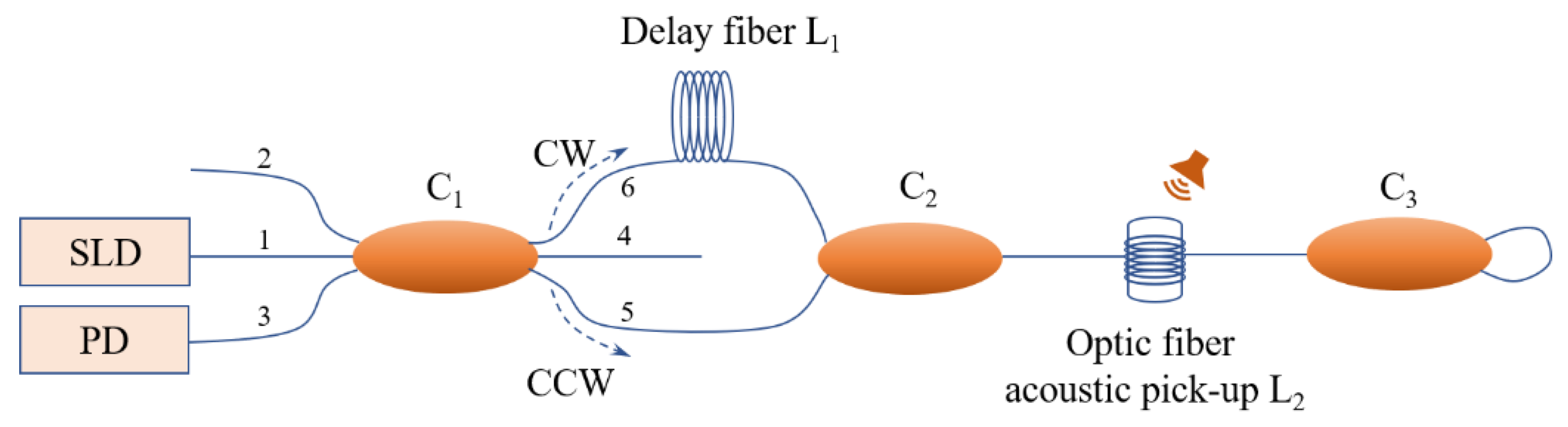
2.1. Sagnac Interference-Based Fiber Optic Acoustic Sensing Principle
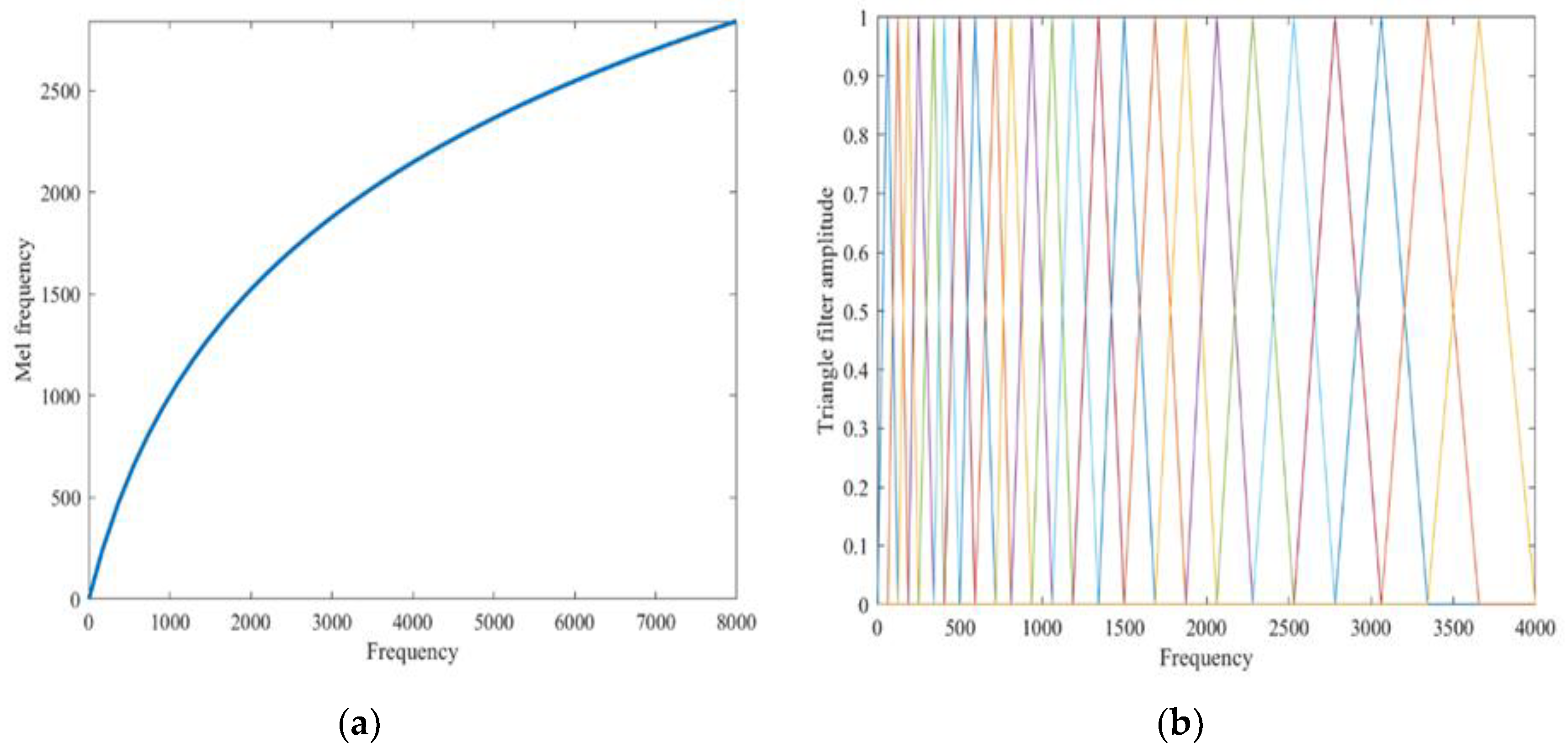
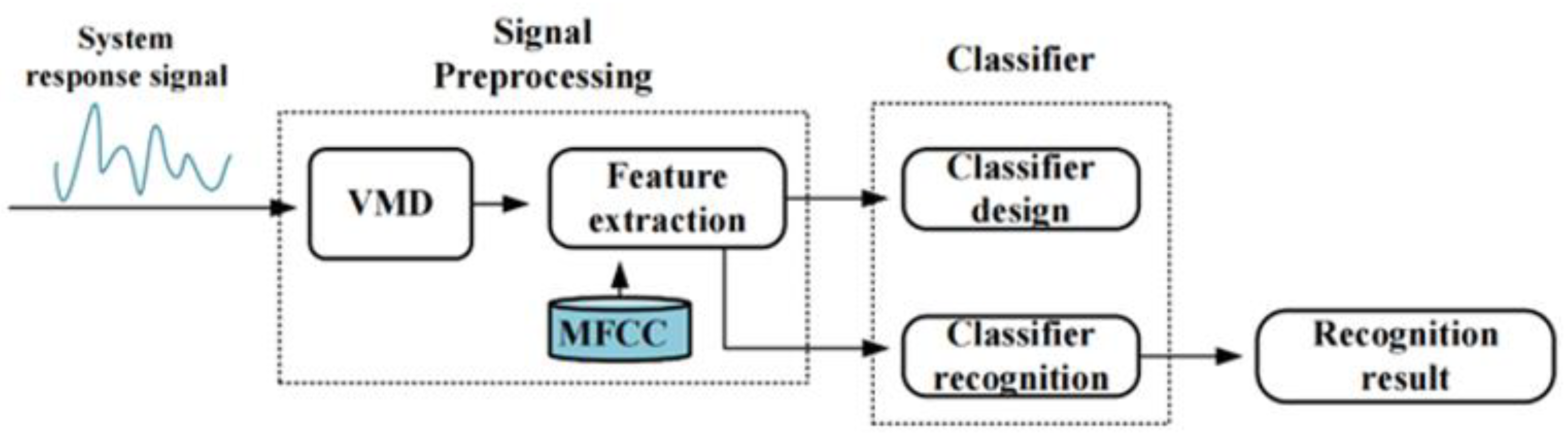
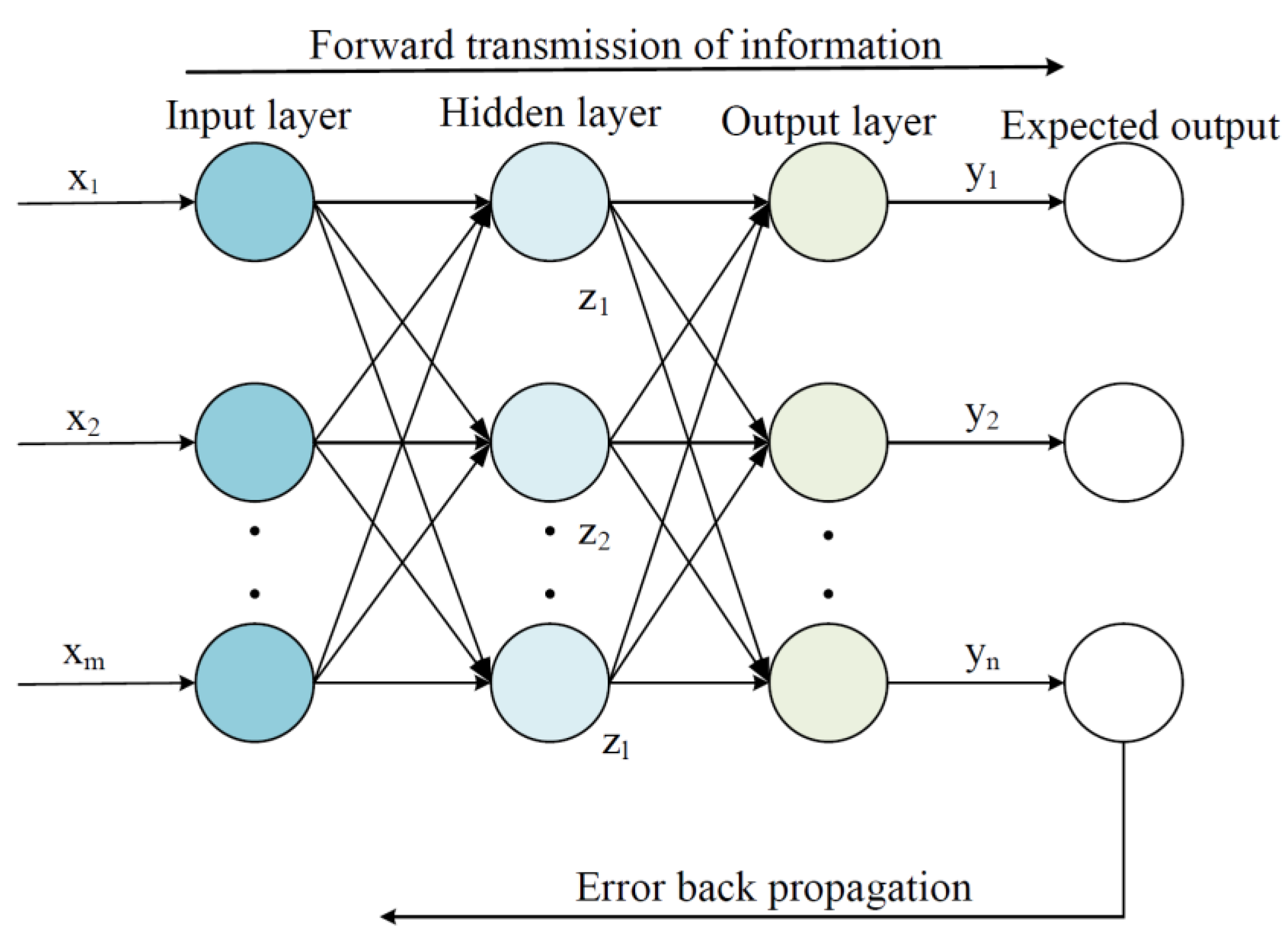
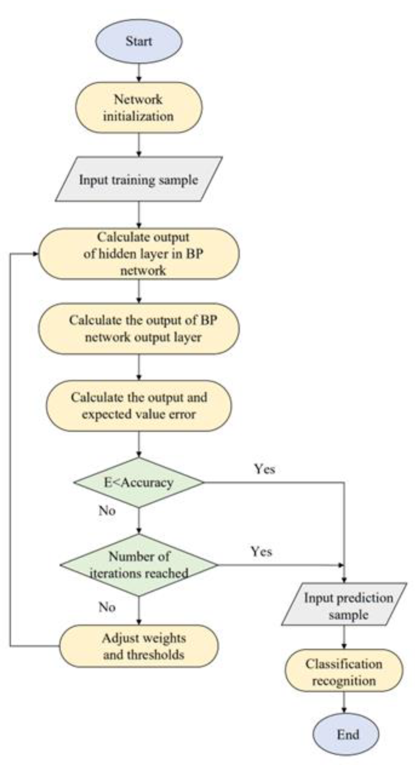
2.2. Optical and Acoustic Signal Recognition Algorithm Design
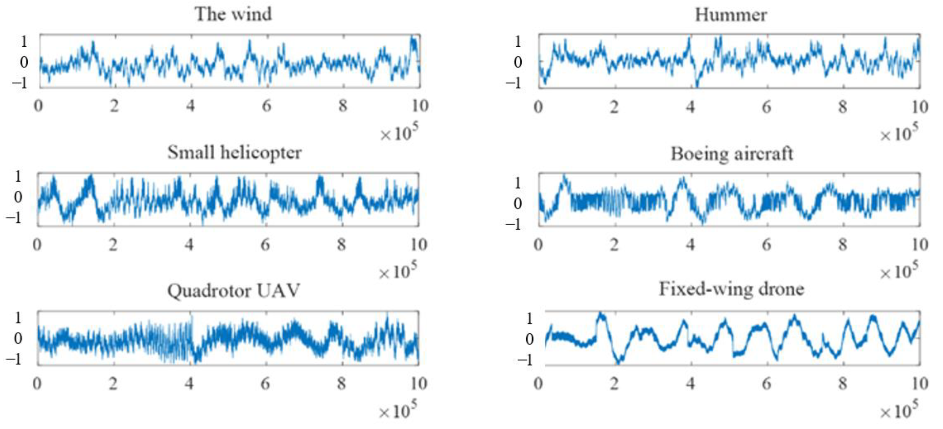
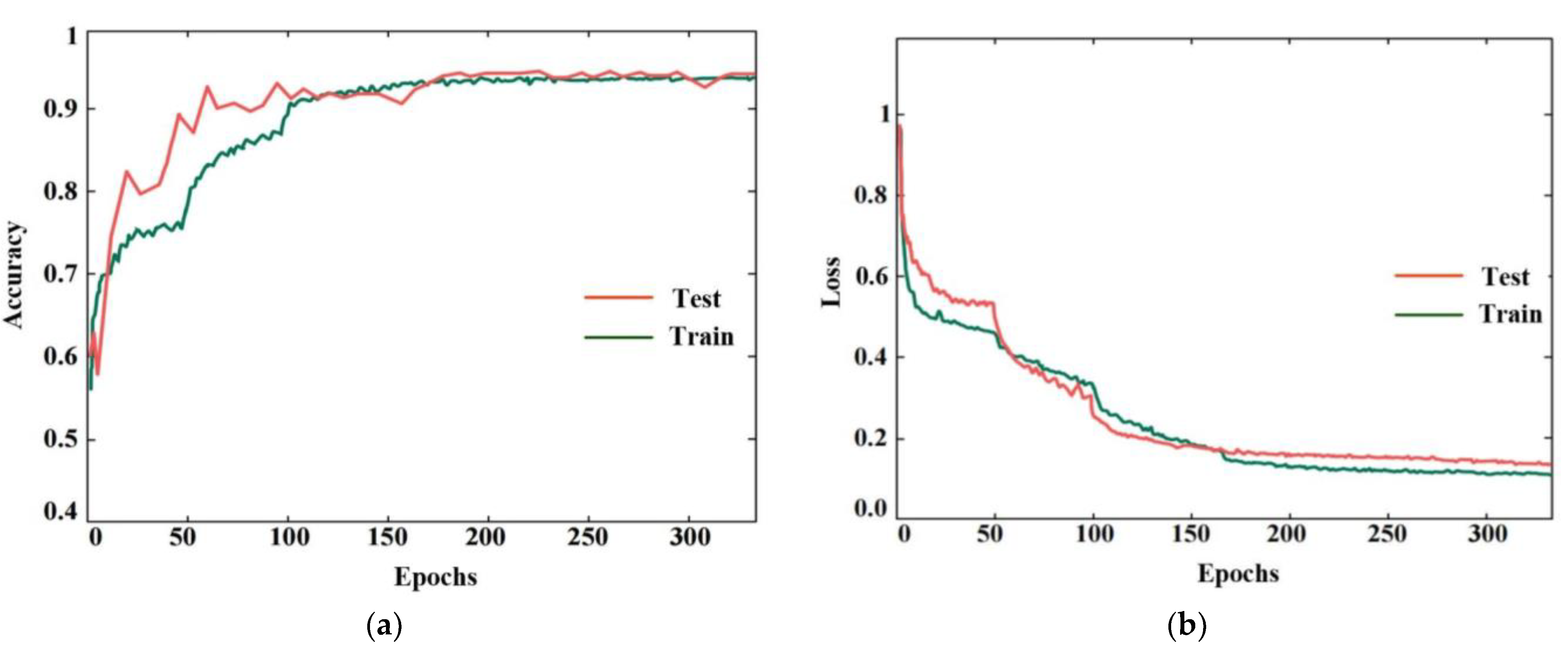
3. Experiment
4. Conclusions
Author Contributions
Funding
Institutional Review Board Statement
Informed Consent Statement
Data Availability Statement
Conflicts of Interest
References
- Lyu, C.; Jiang, J.; Li, B.; Huo, Z.; Yang, J. Abnormal events detection based on RP and inception network using distributed optical fiber perimeter system. Opt. Lasers Eng. 2020, 137, 106377. [Google Scholar] [CrossRef]
- Li, Z.; Zhang, J.; Wang, M.; Zhong, Y.; Peng, F. Fiber distributed acoustic sensing using convolutional long short-term memory network: A field test on high-speed railway intrusion detection. Opt. Express 2020, 28, 2925–2938. [Google Scholar] [CrossRef]
- Zhan, Y.; Song, Z.; Sun, Z.; Yu, M.; Guo, A.; Feng, C.; Zhong, J. A distributed optical fiber sensor system for intrusion detection and location based on the phase-sensitive OTDR with remote pump EDFA. Optik 2020, 225, 165020. [Google Scholar] [CrossRef]
- Zhang, G.; Zhang, W.; Gui, L.; Li, S.; Fang, S.; Zuo, C.; Wu, X.; Yu, B. Ultra-sensitive high temperature sensor based on a PMPCF tip cascaded with an ECPMF Sagnac loop. Sens. Actuators A Phys. 2020, 314, 112219. [Google Scholar] [CrossRef]
- Petrie, C.M.; McDuffee, J.L. Liquid level sensing for harsh environment applications using distributed fiber optic temperature measurements. Sens. Actuators A Phys. 2018, 282, 114–123. [Google Scholar] [CrossRef]
- Xu, J.; Tang, X.; Xin, L.; Sun, Z.; Ning, T. High sensitivity magnetic field sensor based on hybrid fiber interferometer. Opt. Fiber Technol. 2023, 78, 103321. [Google Scholar] [CrossRef]
- Bao, J.; Mo, J.; Xu, L. VMD-based vibrating fiber system intrusion signal recognition. Opt.—Int. J. Light Electron Opt. 2020, 205, 163753. [Google Scholar] [CrossRef]
- Wang, N.; Fang, N.; Wang, L. Intrusion recognition method based on echo state network for optical fiber perimeter security systems. Opt. Commun. 2019, 451, 301–306. [Google Scholar] [CrossRef]
- Ren, Z.; Yao, J.; Huang, Y. High-performance railway perimeter security system based on theinline time-division multiplexing fiber Fabry-Perot interferometricsensor array. Opt.—Int. J. Light Electron Opt. 2022, 249, 168191. [Google Scholar] [CrossRef]
- Wang, J.; Tang, R.; Chen, J.; Wang, N.; Zhu, Y.; Zhang, J.; Ruan, J. Study of Straight-Line-Type Sagnac Optical Fiber Acoustic Sensing System. Photonics 2023, 10, 83. [Google Scholar] [CrossRef]
- Chen, J.; Wang, J.; Wang, N. An Improved Acoustic Pick-Up for Straight Line-Type SagnacFiber Optic Acoustic Sensing System. Sensors 2022, 22, 8193. [Google Scholar] [CrossRef]
- Chen, P.; You, C.; Ding, P. Event classification using improved salp swarm algorithm based probabilistic neural network in fiber-optic perimeter intrusion detectionsystem. Opt. Fiber Technol. 2020, 56, 102182. [Google Scholar] [CrossRef]
- Dragomiretskiy, K.; Zosso, D. Variational mode decomposition. IEEE Trans. Signal Process. 2014, 62, 531–544. [Google Scholar] [CrossRef]
- Liu, B.; Jiang, Z.; Nie, W.; Ran, Y.; Lin, H. Research on leak location method of water supply pipeline based on negative pressure wave technology and VMD algorithm. Measurement 2021, 186, 110235. [Google Scholar] [CrossRef]
- Chen, S.; Li, Y.; Huang, L.; Yin, H.; Zhang, J.; Song, Y.; Wang, M. Vehicle identification based on Variational Mode Decomposition in phase sen-sitive optical time-domain reflectometer. Opt. Fiber Technol. 2020, 60, 102374. [Google Scholar] [CrossRef]
- Liu, K.; Sun, Z.; Jiang, J.; Ma, P.; Wang, S.; Weng, L.; Xu, Z.; Liu, T. A Combined Events Recognition Scheme Using Hybrid Features in Distributed Optical Fiber Vibration Sensing System. IEEE Access 2019, 7, 105609–105616. [Google Scholar] [CrossRef]
- Zhao, Z.; Wang, H.; Huang, Y.; Yao, H.; Li, N.; Tan, H.; Liu, Y. Research on non-invasive load identification method based on VMD. Energy Rep. 2023, 9, 460–469. [Google Scholar] [CrossRef]
- Anwar, M.Z.; Kaleem, Z.; Jamalipour, A. Machine Learning Inspired Sound-Based Amateur Drone Detection for Public Safety Applications. IEEE Trans. Veh. Technol. 2019, 68, 2526–2534. [Google Scholar] [CrossRef]
- Ghaffar, M.S.B.A.; Khan, U.S.; Iqbal, J.; Rashid, N.; Hamza, A.; Qureshi, W.S.; Tiwana, M.I.; Izhar, U. Improving classification performance of four class FNIRS-BCI using Mel Frequency Cepstral Coefficients (MFCC). Infrared Phys. Technol. 2020, 112, 103589. [Google Scholar] [CrossRef]
- Ks, D.R.; Rudresh, G.S. Comparative performance analysis for speech digit recognition based on MFCC and vector quantization. Glob. Transit. Proc. 2021, 2, 513–519. [Google Scholar] [CrossRef]
- Zhang, H.; Mcloughlin, I.; Yan, S. Robust sound event classification using deep neural networks. IEEE/ACM Transactions on Audio. Speech Lang. Process. (TASLP) 2015, 23, 540–552. [Google Scholar]
- Liu, L.; Lu, P.; Liao, H. Fiber-optic michelson interferometric acoustic sensor based on a PP/PET diaphragm. IEEE Sens. J. 2016, 16, 3054–3058. [Google Scholar] [CrossRef]
- Song, S.; Xiong, X.; Wu, X. Modeling the SOFC by BP neural network algorithm. Int. J. Hydrogen Energy 2021, 46, 20065–20077. [Google Scholar] [CrossRef]
- Li, B.; Shen, L.; Zhao, Y.; Yu, W.; Lin, H.; Chen, C.; Li, Y.; Zeng, Q. Quantification of interfacial interaction related with adhesive membrane fouling by genetic algorithm back propagation (GABP) neural network. J. Colloid Interface Sci. 2023, 640, 110–120. [Google Scholar] [CrossRef]
- Muruganandam, S.; Joshi, R.; Suresh, P.; Balakrishna, N.; Kishore, K.H.; Manikanthan, S.V. A deep learning-based feed forward artificial neural network to predict the K-barriers for intrusion detection using a wireless sensor network. Meas. Sens. 2023, 25, 100613. [Google Scholar] [CrossRef]


| Number of Experiment | Small Helicopter (%) | Boeing Aircraft (%) | Hummer (%) | The Wind (%) | Quadrotor UAV (%) | Fixed-Wing Drone (%) | Average Accurancy (%) |
|---|---|---|---|---|---|---|---|
| ① | 100 | 95.74 | 94.64 | 97.06 | 94.87 | 96.97 | 96.40 |
| ② | 100 | 94.29 | 97.5 | 92.31 | 97.62 | 97.44 | 96.53 |
| ③ | 96.33 | 93.10 | 96.55 | 95.45 | 100 | 97.44 | 96.31 |
| ④ | 94.23 | 95.74 | 90.91 | 94.12 | 97.22 | 100 | 96.00 |
| ⑤ | 95.45 | 97.92 | 96.02 | 92.59 | 97.62 | 97.83 | 97.28 |
| First Time/s | Second Time/s | Third Time/s | Fourth Time/s | |
|---|---|---|---|---|
| BP neural network training | 40 | 43 | 43 | 42 |
| BP neural network recognition | 6 | 5 | 5 | 5.3 |
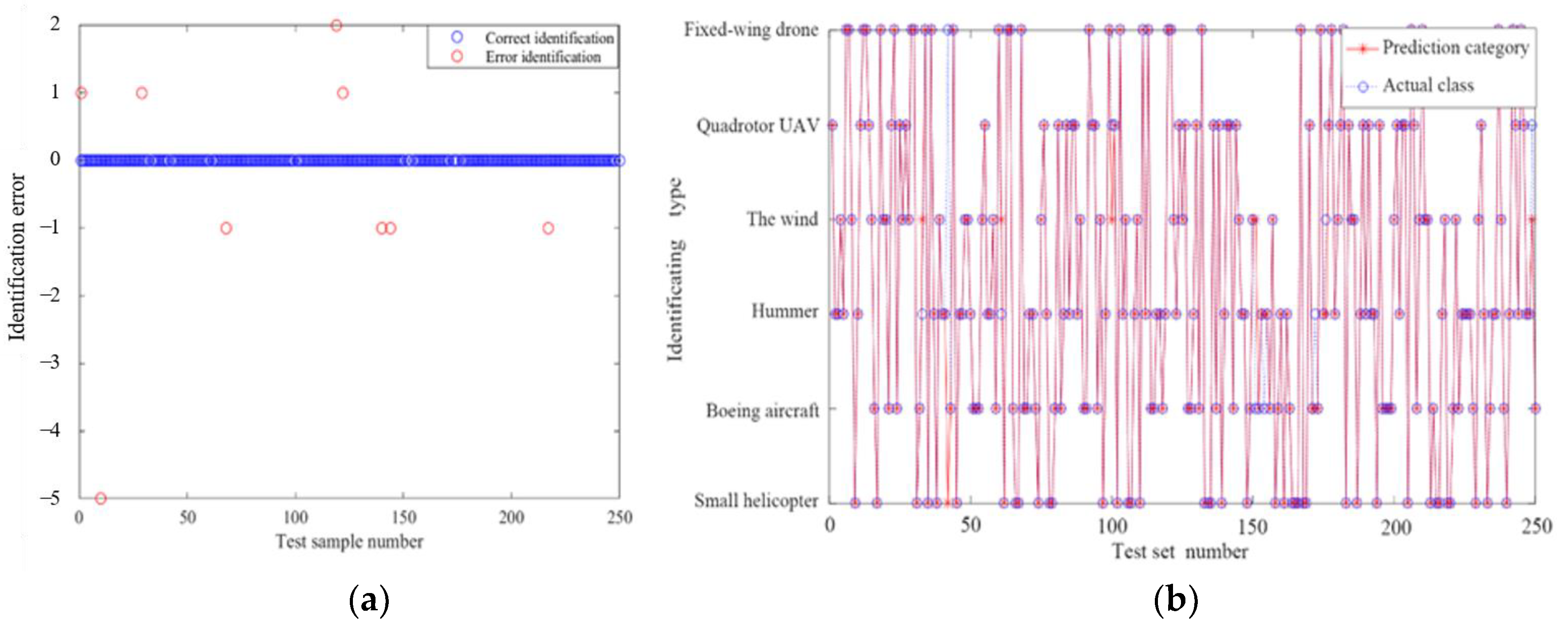
| Data Number | Actual Label | Predictive Label | Data Number | Actual Label | Predictive Label |
|---|---|---|---|---|---|
| 33 | Hummer | The wind | 154 | Boeing aircraft | Hummer |
| 42 | Fixed-wing drone | Small helicopter | 172 | Hummer | Boeing aircraft |
| 61 | Hummer | The wind | 176 | The wind | Hummer |
| 100 | Quadrotor UAV | The wind | 249 | Quadrotor UAV | The wind |
| 151 | Boeing aircraft | The wind |
Disclaimer/Publisher’s Note: The statements, opinions and data contained in all publications are solely those of the individual author(s) and contributor(s) and not of MDPI and/or the editor(s). MDPI and/or the editor(s) disclaim responsibility for any injury to people or property resulting from any ideas, methods, instructions or products referred to in the content. |
© 2023 by the authors. Licensee MDPI, Basel, Switzerland. This article is an open access article distributed under the terms and conditions of the Creative Commons Attribution (CC BY) license (https://creativecommons.org/licenses/by/4.0/).
Share and Cite
Zheng, X.; Tang, R.; Wang, J.; Lin, C.; Chen, J.; Wang, N.; Zhu, Y.; Ruan, J. Research on Multi-Source Simultaneous Recognition Technology Based on Sagnac Fiber Optic Sound Sensing System. Photonics 2023, 10, 1003. https://doi.org/10.3390/photonics10091003
Zheng X, Tang R, Wang J, Lin C, Chen J, Wang N, Zhu Y, Ruan J. Research on Multi-Source Simultaneous Recognition Technology Based on Sagnac Fiber Optic Sound Sensing System. Photonics. 2023; 10(9):1003. https://doi.org/10.3390/photonics10091003
Chicago/Turabian StyleZheng, Xinyu, Ruixi Tang, Jiang Wang, Cheng Lin, Jianjun Chen, Ning Wang, Yong Zhu, and Juan Ruan. 2023. "Research on Multi-Source Simultaneous Recognition Technology Based on Sagnac Fiber Optic Sound Sensing System" Photonics 10, no. 9: 1003. https://doi.org/10.3390/photonics10091003
APA StyleZheng, X., Tang, R., Wang, J., Lin, C., Chen, J., Wang, N., Zhu, Y., & Ruan, J. (2023). Research on Multi-Source Simultaneous Recognition Technology Based on Sagnac Fiber Optic Sound Sensing System. Photonics, 10(9), 1003. https://doi.org/10.3390/photonics10091003