Prediction of Process Parameters for Ultra-Precision Optical Processing Based on Dual-Stacked LSTM

Abstract

High-precision and large-aperture optical components have important applications in modern optics and optoelectronics. However, the traditional continuous polishing technology of optical components relies heavily on the processing experience of the processing personnel. The surface shape of the pitch lap is judged by frequent offline measurement of the surface shape of the processing workpiece, and then the processing personnel judges how to adjust the next process parameters through their own experience, which leads to uncertainty of processing time and low processing efficiency. In this paper, based on the historical processing data, including the surface parameters of workpieces and process parameters before and after each processing, a machine learning-based prediction method of process parameters is proposed. At first, taking the surface shape of the pitch lap as the hidden parameter of the model, a time-series mathematical model of the forward and reverse processing processes is constructed. Theoretical and experimental results show that the prediction method in this paper can effectively reduce the processing time and improve the stability of the workpiece quality.

1. Introduction

High-power solid-state laser equipment, such as the LMJ (laser mégajoule) [1,2], GEKKO [3] and so on, require a great number of optical components with large aperture and high surface quality. Continuous polishing technology is an important method to obtain high-precision and low-roughness optical surfaces, especially for the polishing of neodymium-doped phosphate laser glass slabs used as laser amplifiers in those types of equipment [4,5]. The continuous polishing process is always the bottleneck in the processing line of large-aperture optical components, and its manufacturing cost and processing time both account for more than 50% of the entire manufacturing process. At present, one of the important factors limiting the polishing efficiency of large-aperture optical components is the control of the surface shape of workpieces and the pitch lap. The polishing of large-aperture optical components has great uncertainty and lacks theoretical guidance. At present, the selection of process parameters is still mainly based on the experience of processing personnel.

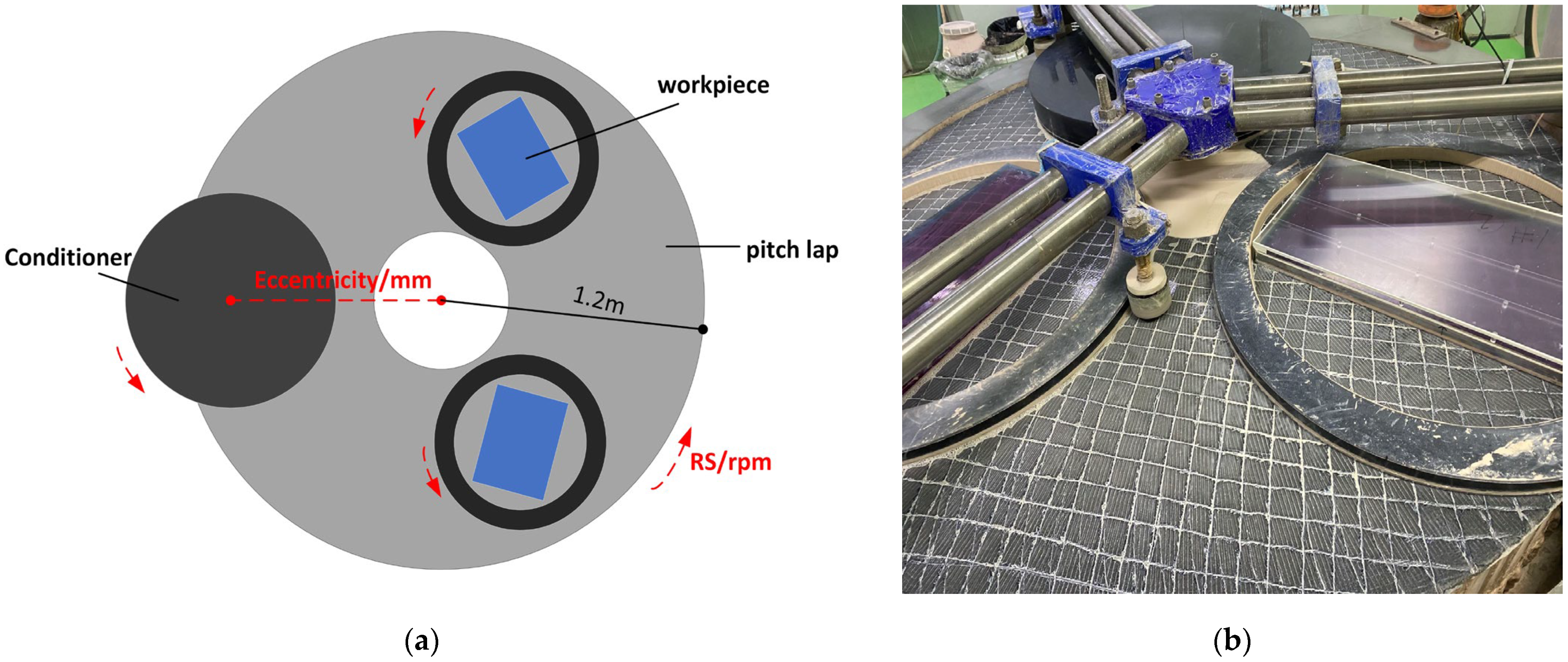
The general structure of the continuous polishing machine is shown in Figure 1. There are two kinds of pitch lap with diameters of 4.4 m and 2.4 m in the workshop. Figure 1 shows a 2.4 m continuous polishing machine. Their materials and working principles are the same. The main difference is that the 4.4 m diameter lap can place four workpieces at the same time, while the 2.4 m diameter lap can only place two workpieces at the same time. The main components of the continuous polishing machine include a circular pitch lap, which is usually poured with asphalt polishing glue (a mixture of asphalt and rosin), or polyurethane, and the thickness of the pitch lap is generally 2–3 cm. The surface of the pitch lap usually has regular grooves, so that the used polishing powder and removed debris can flow out quickly. There will be a certain amount of water in those grooves, which is conducive to dissipating the heat generated by friction. On the pitch lap, there is a circular marble (or glass) conditioner, whose diameter is generally larger than the width of the circular pitch lap, and the position of the conditioner can be adjusted inward or outward relative to the center of the pitch lap.

The eccentricity in Figure 1a is used to describe the position change of the conditioner. Two ferrules are placed on other positions of the pitch lap, and the workpiece is rotated in the ferrule with the polished surface facing down during operation. When the continuous polishing machine is working, the pitch lap is driven at a variable speed by the motor through the power transmission device and rotates at a stable speed (that is, RS in Figure 1a). At the same time, the conditioner and the workpieces on the pitch lap rotate in the same direction for polishing. The workpieces with poor initial surface shape will destroy the surface shape of the pitch lap, which will be repaired by the conditioner. The repaired pitch lap will eventually process a workpiece with high quality, and the relationship between the three is the interaction.

Generally, the processing personnel will remove the workpieces from the pitch lap at regular intervals, clean and wipe them, and then transport them to the testing room. In the testing room that strictly conforms to various testing standards, a large-aperture interferometer [6] is used to detect the reflective surface and transmission surface of the workpieces, and then the results of each test are recorded.

How to improve the continuous polishing technology so as to improve the processing efficiency and the quality of workpieces is mainly focused on the theoretical research of optical processing, mechanics and chemical materials [7,8,9]. The mechanical properties, macro morphology and material characteristics of asphalt pitch lap will directly affect the processing efficiency and the surface shape of workpieces. Therefore, the current research focuses more on the repair method of the surface shape of the pitch lap [10], the influence of the surface characteristics of the pitch lap on the polished surface of the workpiece [11] and the influence of the repair process parameters on the roughness change of the pitch lap before and after the repair [12,13].

This paper studies the prediction of optimal process parameters from the perspective of big data intelligent analysis, that is, through qualitative analysis of historical processing data and real-time optimization of process parameters through mathematical and machine learning models to reduce and replace the dependence on the processing experience of processing personnel. As far as we know, no relevant articles or studies have been found on this point. The main contributions of this paper include:

(1)

Based on the workpiece surface parameters and process parameters before and after processing, a time-series mathematical model of forward and reverse processing processes is constructed, in which the surface shape information of the pitch lap is taken as the hidden parameters of the model;

(2)

A dual-stacked LSTM (long short-term memory) prediction model is proposed to predict process parameters and workpiece surface parameters, respectively. The model implicitly obtains the real-time surface shape information of the pitch lap through the workpiece surface parameters and predicts the real-time optimal process parameters;

(3)

The training and prediction of actual samples show that the prediction method in this paper can effectively improve the prediction accuracy and processing speed.

2. Related Work

2.1. Research on Surface Shape of the Pitch Lap

In the process of continuous polishing, the relationship between the pitch lap and the workpiece is surface contact, which is the contact type of mutual grinding. However, the material of the pitch lap is more wear-resistant and the conditioner can repair the surface of the pitch lap, so the surface shape of the pitch lap will be relatively stable, but as time goes on, the surface shape of the pitch lap is also changing, and the longer the time is, the greater the surface shape change of the pitch lap will be. Therefore, the measurement of the surface shape of the pitch lap is quite important.

Ruiqing Xie et al. put forward a method of measuring the surface shape of the pitch lap in situ in 2018 [14] by installing a sensor-fixed guide rail above the continuous polishing machine, which moves steadily in a straight line along a radius of the pitch lap on the guide rail. Combined with the rotation of the pitch lap itself, the height distribution of the entire pitch lap is obtained through an interpolation algorithm [15], so as to obtain the surface shape characteristics of the pitch lap.

Even if the surface shape characteristics of the pitch lap are accurately measured, the process parameters will still be analyzed and adjusted according to the processing experience of the processing personnel. As the relationship between the optimum process parameters and the shape of the pitch lap is also a complex nonlinear problem, it is uncertain to judge and adjust the process parameters by human experience, which is still a problem to be solved at present.

2.2. Time-Series Prediction Models in Machine Learning

The prediction of process parameters in this paper is a time-series prediction, that is, it needs to predict future data based on historical data, which is essentially a regression prediction. The relevant prediction models in this regard include:

2.2.1. SVR

SVR (support vector regression) is an important application branch of the SVM (support vector machine) [16,17]. It is an application of the SVM to regression problems [18]. However, SVR cannot deal with the time-series data of continuous polishing well and predict the time-series results accurately. LSTM (long short-term memory) and the GRU (gated recurrent unit), as branches of the RNN (recurrent neural network) [19,20,21], can better process and analyze time-series data well.

2.2.2. LSTM

LSTM was first proposed in 1997 and is specially designed to solve the long-term dependency problem of the general RNN [22]. The classical RNN network is mainly to directly splice and combine the hidden layer information at the previous time with the input information and input it into the network at the next time. The expanded RNN in a time sequence is shown in Figure 2 below.

The so-called long-term dependence means that the distance between the useful information and the place where the information needs to be processed is far. After multiple neural network processing, the proportion of the earlier information in the hidden layer information will continue to weaken, which is likely to lead to the RNN being unable to learn the useful information at the far end.

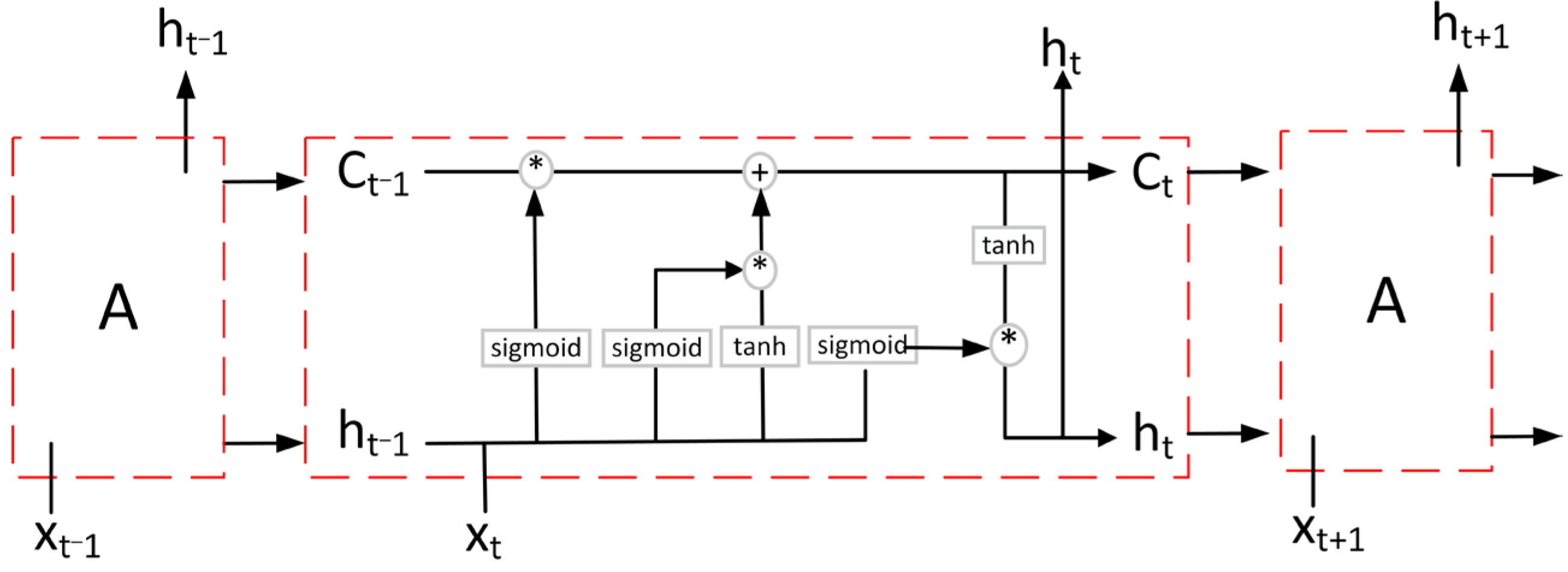
LSTM is carefully designed to avoid long-term dependence, which is the default behavior of LSTM in practice. All RNNs have a chained form of repetitive neural network modules, which have only a very simple structure, such as a Tanh layer. LSTM has the same chained structure, but the repeated modules are different. Unlike the single neural network layer of a RNN, LSTM has four and interacts in a very special way [23], as shown in Figure 3.

Compared with the hidden layer of the original RNN, LSTM adds a cell state [24]. The classic LSTM network structure removes or increases the ability of information to the cell state through a well-designed structure called a “gate”, including a forget gate, an input gate and an output gate.

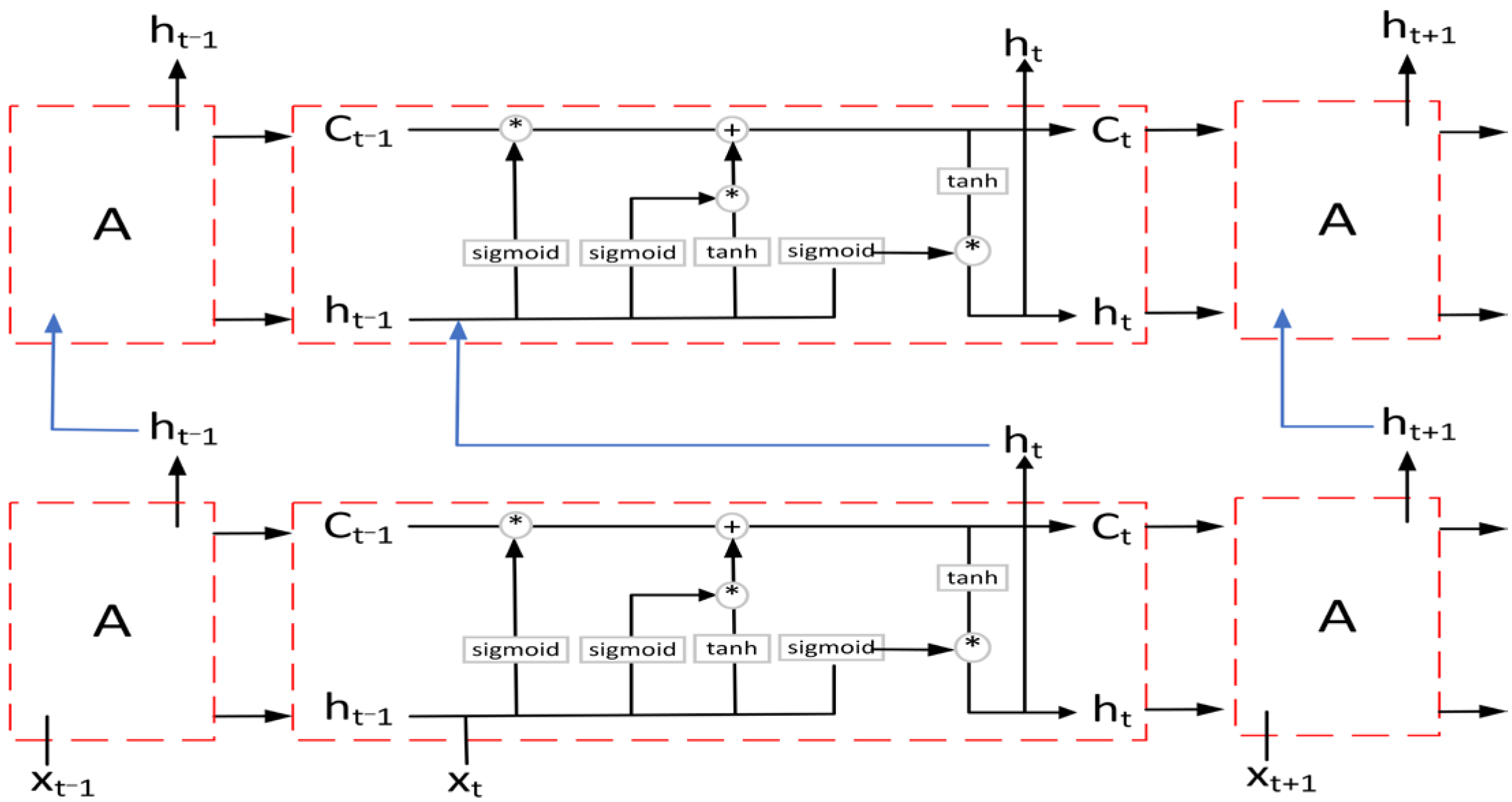
Stacked LSTM is a model composed of multiple LSTM layers stacked with multiple layers. Compared with the single-layer LSTM network structure, stacking multi-LSTM can make the model deeper and the extracted features are more consistent for the nonlinear relationship between input and output. For the stacked LSTM, the output of each time step of the upper layer needs to be taken as the input of the time step of the next layer. Figure 4 shows the network structure diagram of stacking two LSTMs.

2.2.3. GRU

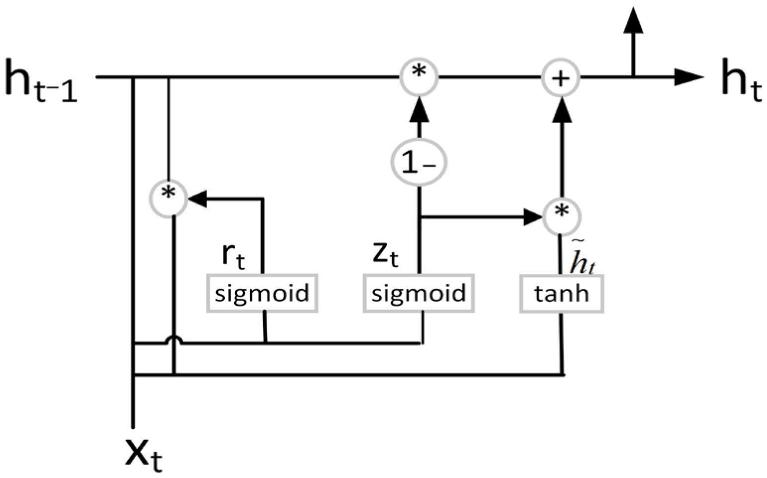
The GRU can also be used to solve the problem of long-term dependence in ordinary RNN networks [25], which was proposed in 2014. It can be regarded as a variant of LSTM. Unlike LSTM, it has only two gate units inside, with a simpler structure and fewer parameters [26]. For the two gates of the GRU, the reset gate determines how to combine the new input information with the previous memory, and the update gate defines the amount of the previous memory saved to the current time step. Its structure is shown in Figure 5.

3. Materials and Methods

During actual processing, the processing personnel frequently take the workpiece off the pitch lap for detection and adjust the process parameters of the next processing through the workpiece parameters and their own processing experience. This may have a serious negative impact; the quality parameters of the workpiece may not change much or even become worse. In addition, the workpieces are frequently taken down and sent to the testing room for measuring; the surface of the workpieces is often knocked or touched, causing damage to the workpieces in this process.

In this paper, the problem of the prediction of process parameters is studied from the perspective of data driving. The complex nonlinear relationship between process parameters, surface shape of the pitch lap and processing results is dynamically learned through the machine learning model, that is, based on historical processing data, including process parameters, and workpiece parameters before and after processing. The surface shape of the pitch lap is implicitly learned through machine learning, and then the best process parameters will be predicted. During processing, it is no longer dominated by the uncertain experience of the processing personnel, but through machine learning to train an appropriate model of prediction, and through the model to adjust the process parameters of each processing, so as to reduce the uncertainty of processing and improve the processing efficiency.

3.1. Parameters and Pretreatment of Model

The historical processing data are recorded in the order of workpiece processing time. The recorded parameters mainly include parameters of the continuous polishing machine, workpiece parameters and environmental parameters. The processing workshop always keeps a constant temperature and humidity, so the influence of environmental parameters on processing is not considered in this paper.

The process parameters include eccentricity, rotational speed (RS) and processing time. Eccentricity is used to indicate the position of the conditioner on its fixed linear track and RS is the rotational speed of the pitch lap. The processing personnel will adjust these three parameters for the next processing according to the detected surface parameters of the workpieces.

The workpiece parameters involved in this paper include peak to valley (PV), power and astigmatism magnitude (astmag). Their unit is the working wavelength (λ) of the interferometer. PV is the peak-valley value of the height of the workpiece surface. Power is used to describe the degree of concavity and convexity of the workpiece surface. Additionally, astmag is used to describe the overall roughness of the workpiece surface. The unit of the workpiece parameter λ is the working wavelength of the interferometer. It is a relative unit. The conversion relationship between the workpiece parameter and the absolute unit is as follows (take PV as an example): PV (nm) = PV (λ) × λ. These three parameters are mainly used to indicate the smoothness and roughness of the workpiece. The closer they are to 0, the smoother the surface of the workpiece is.

3.2. Mathematical Model of Processing Process

Assume that the parameters of the surface shape of the pitch lap are p, which is a vector that changes constantly with the processing process, and is determined by multiple factors such as the material of the pitch lap, workpieces, conditioner and process parameters, with extremely complex nonlinear relationships. The surface parameters of the workpiece before and after processing are, respectively, x and y, including the aforementioned PV, power and astmag. The process parameters are θ, including the aforementioned eccentricity, RS and processing time. The processing process can be modeled as:

$$\mathit{y}(t+1)=f(\mathit{x}(t),\mathit{p}(t),\mathit{\theta }(t),\mathit{\theta }(t+1))$$

(1)

where t is a discrete value, measured in processing times. Mapping f is an extremely complex nonlinear function, which cannot be modeled by accurate models at present. For the data-driven modeling method in this paper, we use a time-series neural network model to fit this function, and the fitting data are the actual measured historical data x(t), y(t+1), θ(t) and θ(t+1).

The solution of Formula (1) faces two problems. First, we need to predict that θ(t+1), but θ(t+1) is the independent variable of Formula (1). To predict θ(t+1), we need to build an inverse function, as shown in Formula (2):

$$\mathit{\theta }(t+1)=g(\mathit{x}(t),\mathit{\theta }(t),\mathit{p}(t),\mathit{y}(t+1))$$

(2)

This also requires a time-series neural network model to fit. Another problem is p(t), which is the surface shape of the pitch lap. We do not know what the p(t) is or how to get it during training. We can express it as a hidden parameter of the neural network, and update and iterate it with the training. Thus, based on the above mathematical modeling, the model of the dual-stacked LSTM is constructed for the prediction of process parameters

3.3. Dual Prediction Model

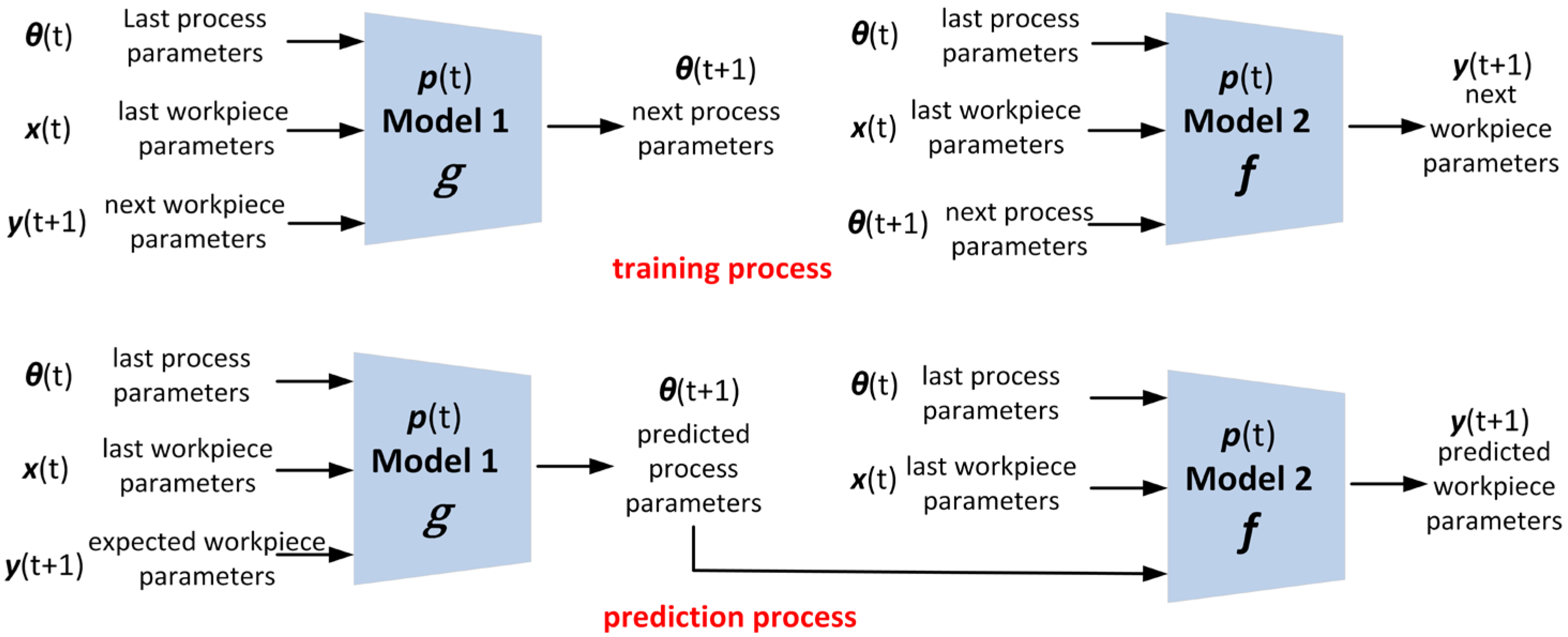
In this paper, the following dual model of prediction is used to train and predict process parameters and workpiece parameters. Model 1 is used to predict the process parameters, and Model 2 is used to predict the workpiece parameters under the process parameters obtained from Model 1. The workpiece parameters predicted by Model 2 will be compared with the actual data for checking the improvement of efficiency brought by process parameters from Model 1. The specific training and prediction process of the dual model of prediction is shown in Figure 6.

Each of these models can be compared and selected among various machine learning models, which are discussed and analyzed in the following experiment section.

4. Experiments and Verification

4.1. Experimental Settings and Datasets

Experimental operating system: Windows10, four core eight threads, RAM(8G), i7 processor, 3.19 GHZ, Microsoft.NET Framework5.0, NVIDIA GEFORCE GTX 1080 Ti graphics card. The experiment is implemented using Pytorch 1.4.0 [27]. The data in the experiment are mainly collected from the processing data of a 4.4 m caliber continuous polishing machine for nearly one and a half years. After sorting out and analyzing, there are 1050 valid data. The 1050 pieces of data are divided into 627 pieces in the T state and 423 pieces in the L state according to the different ways in which the interferometer detects the workpieces. Taking 627 pieces of data in the T state as an example, the test results of dual models trained by different neural network models will be shown. After sorting 627 pieces of data by time, 500 pieces of data are selected as the training set for the training model, and the remaining 127 pieces of data are used as the test set to compare the advantages and disadvantages of different models. We set the epoch to 100, that is, how many times the entire training set has been trained, without considering the premise of the early stop. We set the patience to 10, that is, when you train the epoch, the verification set will stop without advancing. The early stop mechanism is to stop the training to prevent overfitting when the model training has not improved the prediction effect of the verification set for successive periods of patience.

4.2. Experimental Results and Discussion

As shown in the process of prediction in Figure 6, above, the actual data of PV, power, astmag are used as inputs and as the expected workpiece parameters of Model 1 to obtain the predicted process parameters. Then, the process parameters are used as inputs of Model 2 to predict the workpiece parameters after processing through the process parameters given by Model 1. Then, the predicted workpiece parameters are compared with the actual workpiece parameters to check the effectiveness of the model.

In all experiments, the mean square error (MSE) and mean absolute error (MAE) between actual values and predicted values are used to measure the prediction accuracy of the model.

4.2.1. Comparison of Different Machine Learning Models

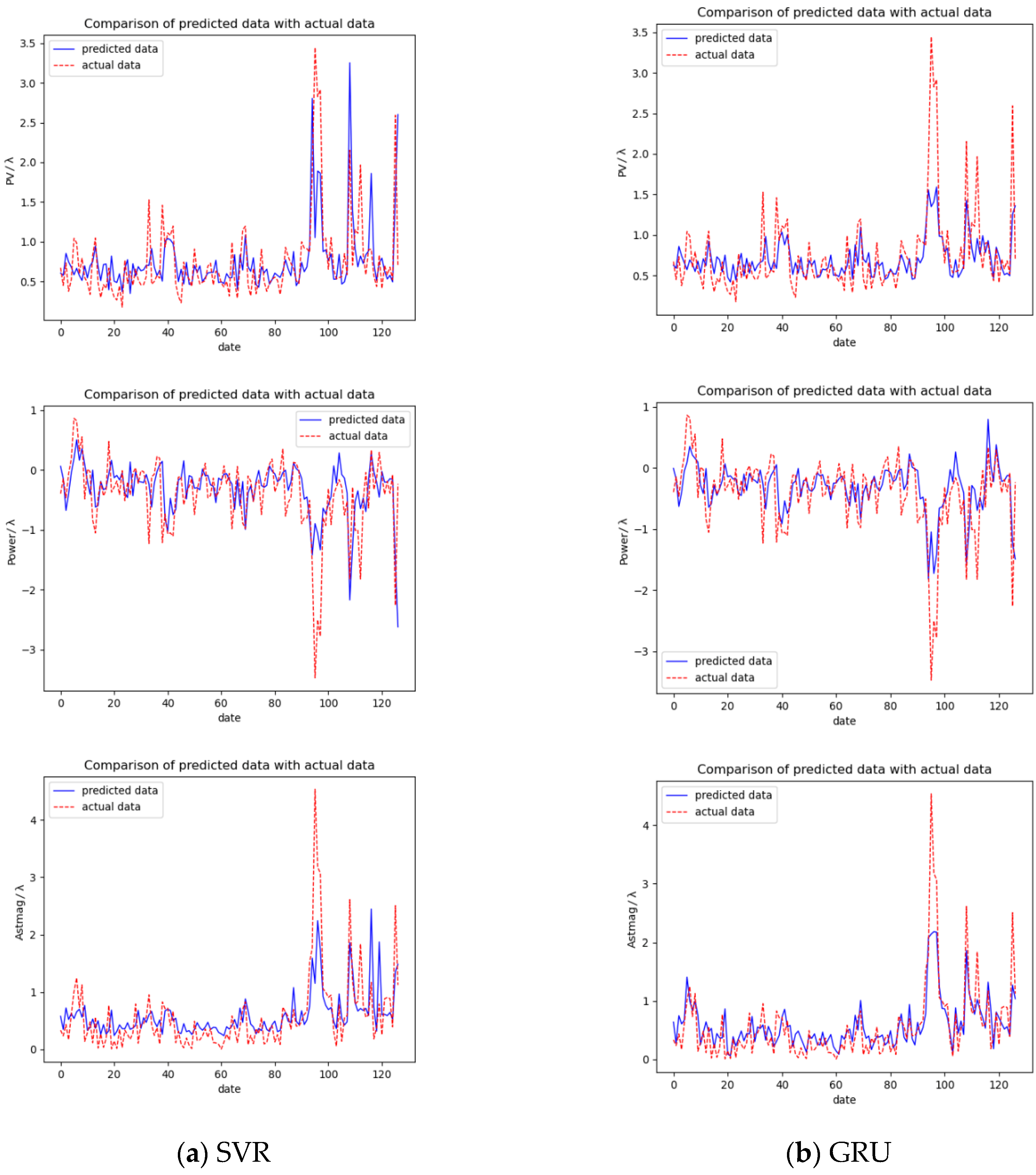
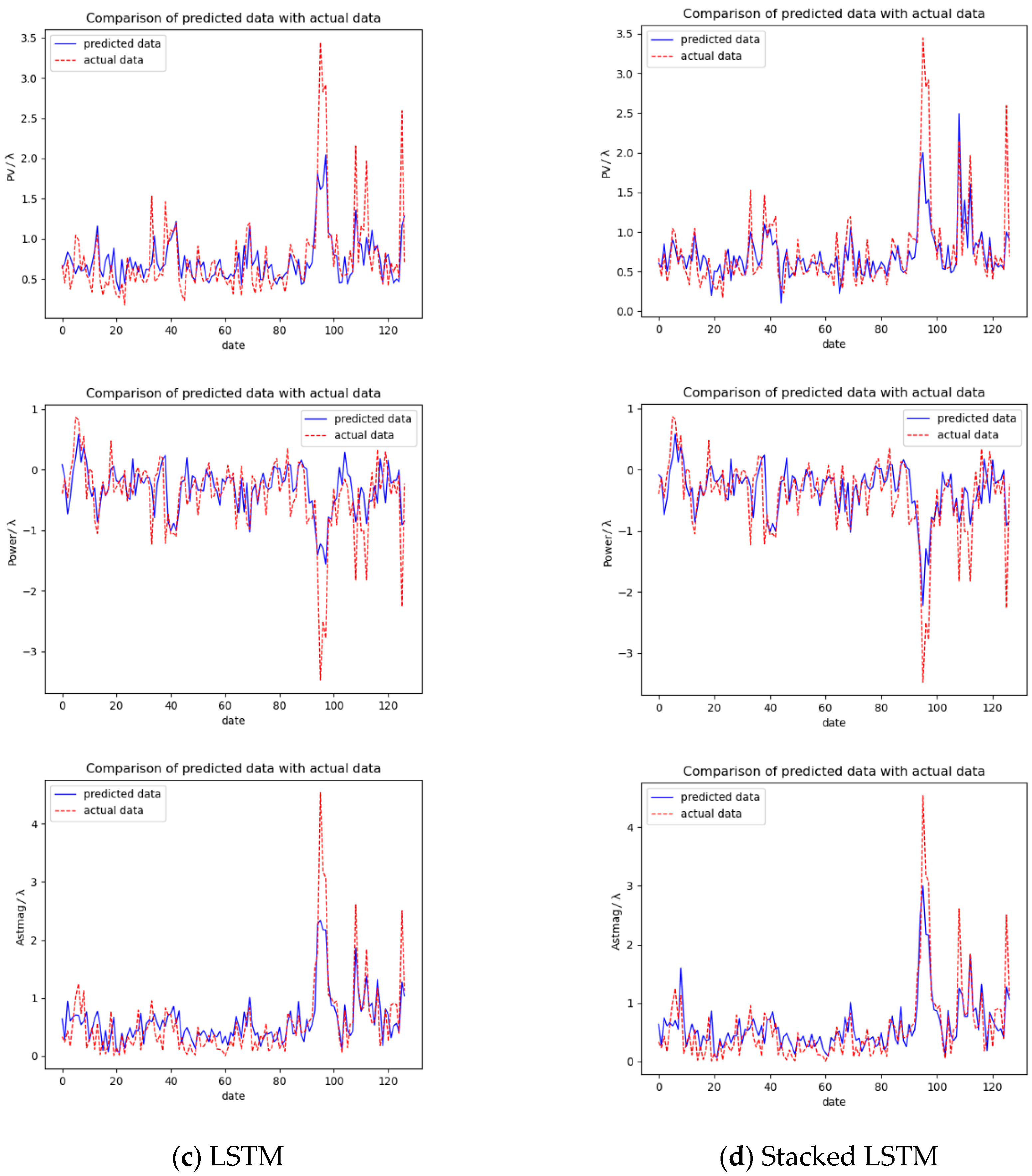
The input data of Model 1 training are θ(t), x(t) and y(t+1) in Figure 6, and the output datum is θ(t+1). The input data of Model 2 training are θ(t), x(t) and θ(t+1) in Figure 1, and the output datum is y(t+1). In the validation, y(t+1) of Model 1 is the actual datum x(t+1). Then, the output processing parameter and then the processing parameter are obtained as the input of Model 2. The output workpiece parameter is obtained and the workpiece parameter and the actual data are compared to get the pros and cons of each model. The experiment mainly compares the advantages and disadvantages of SVR, GRU, LSTM and stacked LSTM models. The comparison results are as follows.

It can be seen from Figure 7 that the model trained by stacking three layers of LSTM has the best-fitting effect. Additionally, the peak is likely to be due to the worker’s judgment error, and the adjustment of processing parameters is unreasonable, resulting in the workpiece surface shape parameters becoming worse after processing. As shown in

Table 1. Mean square error and mean absolute error of PV on different modules.

Error	SVR	GRU	LSTM	Stacked LSTM
MSE/λ2	0.1886	0.1463	0.1268	0.1065
MAE/λ2	0.2643	0.2388	0.2265	0.1992

,

Table 2. Mean square error and mean absolute error of power on different modules.

Error	SVR	GRU	LSTM	Stacked LSTM
MSE/λ2	0.2765	0.2162	0.2204	0.1854
MAE/λ2	0.3399	0.3209	0.3184	0.2990

and

Table 3. Mean square error and mean absolute error of astmag on different modules.

Error	SVR	GRU	LSTM	Stacked LSTM
MSE/λ2	0.2302	0.1485	0.1478	0.1387
MAE/λ2	0.2964	0.2547	0.2665	0.2566

, the minimum error is bolded. Generally speaking, stacked LSTM performs the best. Among the six errors of three workpiece parameters, five errors of stacked LSTM are the smallest. However, the difference between the several models is not particularly obvious. In addition to the similar structure of LSTM and the GRU, we believe that staked LSTM will be more obvious with the continuous increase in processing data and the continuous training and iteration of the model. Of course, this is the part we will continue to optimize later.

4.2.2. Comparison of Different Time Steps of LSTM

From the above

Table 4. Mean square error and mean absolute error of PV on different time steps.

Error	10	15	20	30
MSE/λ2	0.1366	0.1065	0.1031	0.1245
MAE/λ2	0.2243	0.1992	0.1879	0.2014

,

Table 5. Mean square error and mean absolute error of Power on different time steps.

Error	10	15	20	30
MSE/λ2	0.2038	0.1854	0.1653	0.1721
MAE/λ2	0.3304	0.2990	0.2567	0.2533

and

Table 6. Mean square error and mean absolute error of astmag on different time steps.

Error	10	15	20	30
MSE/λ2	0.1638	0.1387	0.1251	0.1366
MAE/λ2	0.2643	0.2566	0.2317	0.2433

, we know that the best prediction effect will be obtained when the time step of the model is set to 20, which indicates that the surface shape of the pitch lap is actually related to the previous 20 times of processing.

4.3. Verification

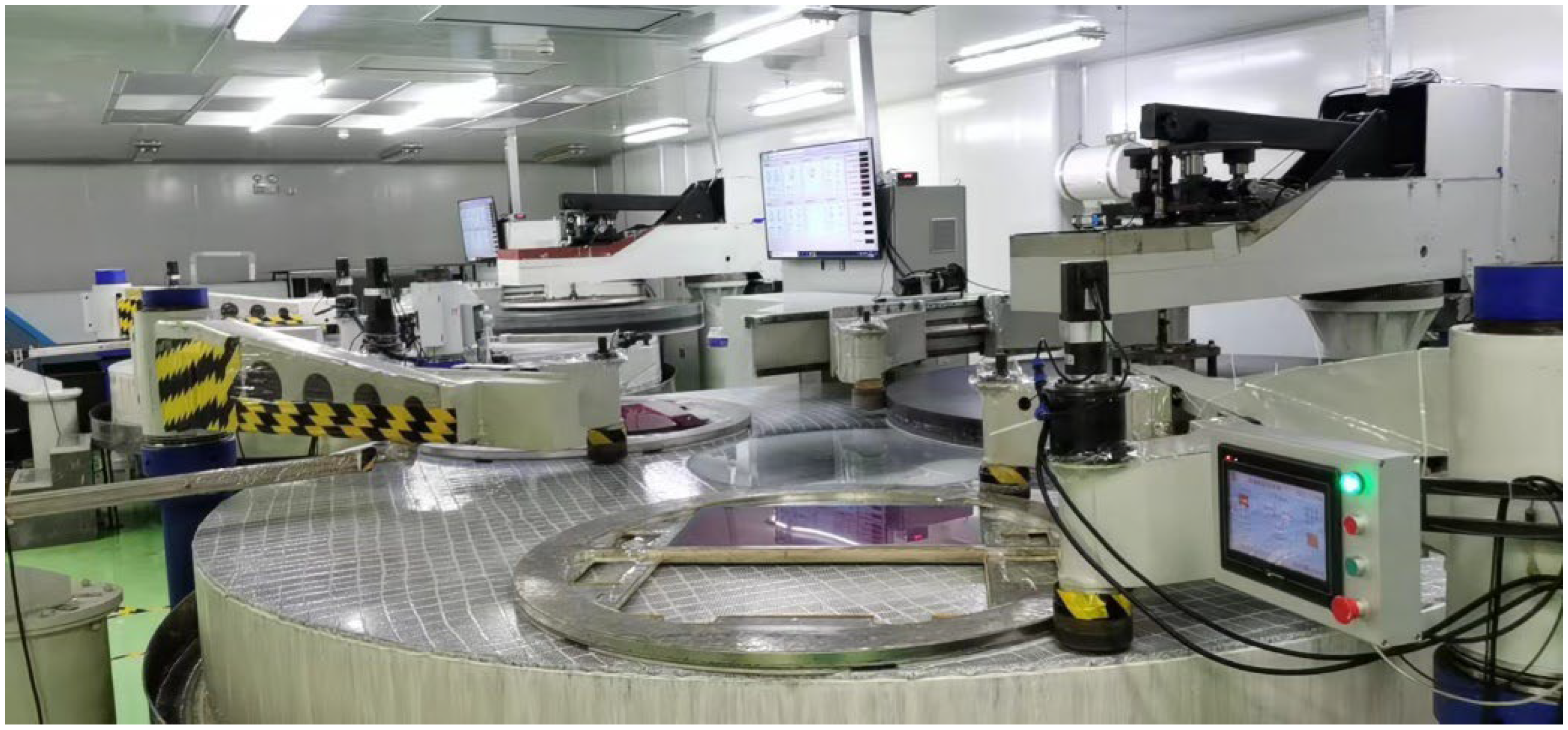
The dataset in the previous section was collected from a 4.4 m caliber continuous polishing machine in the workshop, which we named 2#. The verification test was also carried out on this continuous polishing machine, and each processing parameter was predicted by the dual-stacked LSTM model proposed in this paper. At the same time, another continuous polishing machine named 3# in the same workshop operated normally, and each processing parameter was judged and adjusted by the workers themselves. Continuous polishing machine 2# is shown in Figure 8.

The following

Table 7. Processing yield of machine 2# and machine 3# in August, September, October and November.

Yield	August	September	October	November
2#/pieces	19	20	22	23
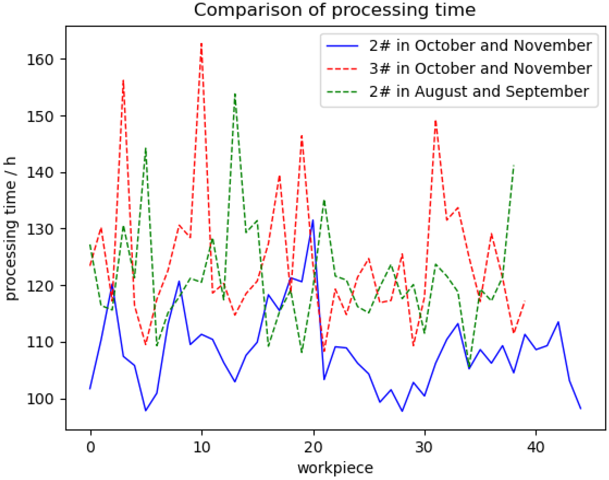
3#/pieces	20	18	19	21

shows the processing yield of machines 2# and 3# in August, September, October and November. The processing parameters of machine 2# in August, September and machine 3# were judged and adjusted by the workers themselves, while the processing parameters of machine 2# in October and November were predicted by the dual-stacked LSTM model.

The average processing times of each workpiece produced by machine 2# in August, September and machine 3# in October and November are 124.3 h and 121.6 h, respectively. The average processing time of each workpiece produced by machine 2# in October and November is 108.6 h, and the efficiency is improved by about 12%. Figure 9 shows the processing time of each workpiece processed by machine 2# and machine 3#.

5. Conclusions

Aiming at the problem that the traditional continuous polishing technology of optical components relies heavily on the experience of the processing personnel, this paper studies the predicted model and method of process parameters based on big data of intelligent analysis and the data-driven method. By recording all processing data of the pitch lap in the past, including the workpiece parameters and process parameters before and after processing, the surface shape of the pitch lap is taken as the hidden parameter of the model, and the mathematical models of the forward and reverse processing processes are constructed. A dual-stacked LSTM prediction model is proposed to predict the process parameters and workpiece parameters, respectively. The model can implicitly obtain the real-time surface shape of the pitch lap through the historical workpiece parameters and predict the real-time optimal process parameters with high accuracy. Through the actual processing test, the processing cycle has been shortened by more than 10%, and the stability of the workpiece quality has been improved, which shows that the dual-stacked LSTM model proposed in this paper effectively improves processing efficiency. In the future, we will further study the optimization of the model and collect more relevant data to obtain better-predicted results.

References

- André, M.L. The French megajoule laser project (LMJ). Fusion Eng. Des. 1999, 44, 43–44. [Google Scholar] [CrossRef]
- Salamin, Y.I.; Hu, S.; Hatsagortsyan, K.Z.; Keitel, C.H. Relativistic high-power laser–matter interactions. Phys. Rep. 2006, 427, 41–155. [Google Scholar] [CrossRef]
- Azechi, H.; Nakai, M.; Shigemori, K.; Miyanaga, N.; Shiraga, H.; Nishimura, H.; Honda, M.; Ishizaki, R.; Wouchuk, J.; Takabe, H.; et al. Direct-drive hydrodynamic instability experiments on the GEKKO XII laser. Phys. Plasmas 1997, 4, 4079–4089. [Google Scholar] [CrossRef]
- Nichols, M. Summary of Synthetic Lap Polishing Experiments at LLNL, FY95; Technical Report; Lawrence Livermore National Lab. (LLNL): Livermore, CA, USA, 2001. [Google Scholar]
- Vijayan, N.; Raj, S.A.; Muthirulan, V.; Sachidananda, K.H. Design and Fabrication of a Continuous Polishing Machine. J. Eur. Des Systèmes Autom. 2019, 52, 485–493. [Google Scholar] [CrossRef]
- Malacara, Z.; Servin, M. Interferogram Analysis for Optical Testing; CRC Press: Boca Raton, FL, USA, 2018. [Google Scholar]
- Nie, X.; Li, S.; Shi, F.; Hu, H. Generalized numerical pressure distribution model for smoothing polishing of irregular midspatial frequency errors. Appl. Opt. 2014, 53, 1020–1027. [Google Scholar] [CrossRef] [PubMed]
- Suratwala, T.; Feit, M.D.; Steele, W.A.; Wong, L.L. Influence of temperature and material deposit on material removal uniformity during optical pad polishing. J. Am. Ceram. Soc. 2014, 97, 1720–1727. [Google Scholar] [CrossRef]
- Cao, C.; Feng, G.; Yang, L.; Wang, F.; Gao, Y.; Zhu, H. Calculation and simulation for the factors affecting relative grinding removal in ultra-precision continuous polishing. Opto-Electron. Eng. 2004, 31, 67–71. [Google Scholar]
- Kim, H.; Kim, H.; Jeong, H.; Seo, H.; Lee, S. Self-conditioning of encapsulated abrasive pad in chemical mechanical polishing. J. Mater. Process. Technol. 2003, 142, 614–618. [Google Scholar] [CrossRef]
- Xie, R.; Li, Y.; Wang, J.; Chen, X.; Huang, H.; Xu, Q. The effect of characteristic of pad on surface form of optical flats in polishing. Opto-Electron. Eng. 2010, 37, 64–69. [Google Scholar]
- Hooper, B.; Byrne, G.; Galligan, S. Pad conditioning in chemical mechanical polishing. J. Mater. Process. Technol. 2002, 123, 107–113. [Google Scholar] [CrossRef]
- Tso, P.L.; Ho, S.Y. Factors influencing the dressing rate of chemical mechanical polishing pad conditioning. Int. J. Adv. Manuf. Technol. 2007, 33, 720–724. [Google Scholar] [CrossRef]
- Xie, R.; Liao, D.; Chen, J.; Zhao, S.; Chen, X.; Ji, B.; Wang, J.; Xu, Q. In-situ shape measurement technology during large aperture optical planar continuous polishing process. In Proceedings of the Young Scientists Forum 2017, SPIE, Shenzhen, China, 4–7 September 2018; Volume 10710, pp. 740–745. [Google Scholar]
- Liao, D.; Zhang, Q.; Xie, R.; Chen, X.; Zhao, S.; Wang, J. Deterministic measurement and correction of the pad shape in full-aperture polishing processes. J. Eur. Opt. Soc. -Rapid Publ. 2015, 10. Available online: https://www.jeos.org/index.php/jeos_rp/article/view/15049 (accessed on 5 February 2023). [CrossRef]
- Noble, W.S. What is a support vector machine? Nat. Biotechnol. 2006, 24, 1565–1567. [Google Scholar] [CrossRef] [PubMed]
- Suthaharan, S. Machine learning models and algorithms for big data classification. Integr. Ser. Inf. Syst. 2016, 36, 1–12. [Google Scholar]
- Smola, A.J.; Schölkopf, B. A tutorial on support vector regression. Stat. Comput. 2004, 14, 199–222. [Google Scholar] [CrossRef]
- Zaremba, W.; Sutskever, I.; Vinyals, O. Recurrent neural network regularization. arXiv 2014, arXiv:1409.2329. [Google Scholar]
- Medsker, L.R.; Jain, L. Recurrent neural networks. Des. Appl. 2001, 5, 64–67. [Google Scholar]
- Schmidhuber, J. Deep learning in neural networks: An overview. Neural Netw. 2015, 61, 85–117. [Google Scholar] [CrossRef]
- Hochreiter, S.; Schmidhuber, J. Long short-term memory. Neural Comput. 1997, 9, 1735–1780. [Google Scholar] [CrossRef]
- Graves, A. Supervised sequence labelling. In Supervised Sequence Labelling with Recurrent Neural Networks; Springer: Berlin/Heidelberg, Germany, 2012; pp. 5–13. [Google Scholar]
- Van Houdt, G.; Mosquera, C.; Nápoles, G. A review on the long short-term memory model. Artif. Intell. Rev. 2020, 53, 5929–5955. [Google Scholar] [CrossRef]
- Cho, K.; Van Merriënboer, B.; Gulcehre, C.; Bahdanau, D.; Bougares, F.; Schwenk, H.; Bengio, Y. Learning phrase representations using RNN encoder-decoder for statistical machine translation. arXiv 2014, arXiv:1406.1078. [Google Scholar]
- Chung, J.; Gulcehre, C.; Cho, K.; Bengio, Y. Empirical evaluation of gated recurrent neural networks on sequence modeling. arXiv 2014, arXiv:1412.3555. [Google Scholar]
- Paszke, A.; Gross, S.; Chintala, S.; Chanan, G.; Yang, E.; DeVito, Z.; Lin, Z.; Desmaison, A.; Antiga, L.; Lerer, A. Automatic differentiation in pytorch. 2017. Available online: https://openreview.net/forum?id=BJJsrmfCZ (accessed on 5 February 2023).