Method for the Quantum Metric Tensor Measurement in a Continuous Variable System

Abstract

As a fundamental concept, geometry is widely used in understanding physical phenomena. In quantum mechanics, geometry is related to the system’s quantum state and can be characterized by the quantum geometric tensor (QGT), whose real part is referred to as the quantum metric tensor (QMT), which defines the distance between two neighboring quantum states in the projected Hilbert space. Several pieces of research based on discrete variables have been proposed to extract the QMT, but research with the use of continuous variables is lacking. Here, we propose a method to extract the QMT of a continuous variable system, specified here as a cat-qubit. The method is developed by constructing the Kerr nonlinear parametric oscillator (KNPO) and by modulating it with external drives to induce adiabatic dynamics process within the state subspace spanned by the even and odd $Sch\ddot{o}dinger$ cat states. The method paves the way for exploring the geometry for continuous variable systems.

1. Introduction

Geometry is a critical concept for describing fundamental principles of nature. In the quantum world, quantum states are presented by the wavefunctions in Hilbert space with specific dimensions, quantum geometry builds the geometric construction in this space [1,2,3].

The quantum geometric tensor (QGT) [4,5,6,7,8] provides a powerful tool to outline the geometry of Hilbert space. On one hand, its imaginary part, Berry curvature, is widely explored for understanding various physical phenomena, such as the Aharonov–Bohm effect [9], the Berry phase [10,11,12,13,14] and the topology of condensed matter [15,16,17,18,19,20]. On the other hand, the real part defines the quantum metric tensor (QMT), which reflects the quantum distance between two neighboring quantum states in the parametric space. What is more, as a gauge invariable, the QMT has been widely exploited in various studies, such as quantum fluctuations [21,22,23,24], quantum phase transition [25,26,27,28,29] and topological matter [30]. It is also associated with a topological invariant, the Euler characteristic number [2,6,31,32,33], for describing the topology of the state manifold. So, it is pivotal to measure the QMT for analyzing the geometry of the quantum system.

So far, theoretical and experimental studies have been conducted to measure the QMT in different physical systems [33,34,35,36,37,38,39,40,41]. However, schemes to measure this intriguing quantity in a continuous variable system are still lacking. Here, we propose a scheme to measure the QMT in a continuous variable system with cat-qubit encoding [42,43,44,45,46]. We consider a superconducting quantum interference device (SQUID) array [47] to construct the Kerr nonlinear parametric oscillator (KNPO) [48,49,50,51,52] for stabilizing the Schr$\ddot{o}$dinger cat states, together by inducing two modulated drives and controlling the detuning of the oscillator to realize an effective and modulated two-level system, with a pair of continuous variable even and odd schr$\ddot{o}$dinger cat states as the encoding bases. Through the method of adiabatic control of the KNPO system’s state evolution in the parametric space, we numerically analyze and extract the QMT. The results are highly consistent with the theory, providing an effective method with which to explore the geometry of continuous variable systems.

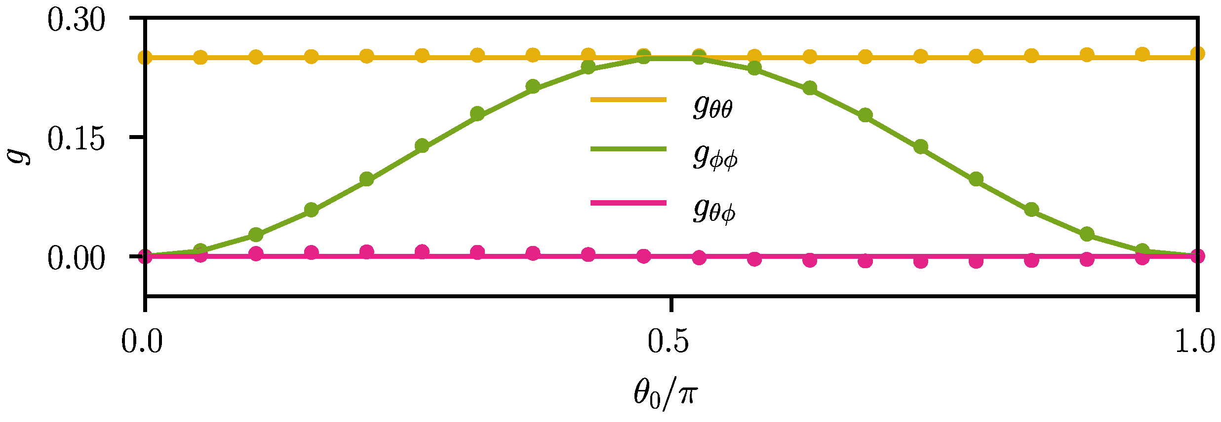
2. Quantum Metric Tensorl (QMT)

We consider a Hamiltonian $\widehat{H}(\mathbf{r})$ of a nondegenerate quantum system, which is dependent on N dimensionless parameters $\mathbf{r}={(r_1,r_2,\dots ,r_N)}^{Tr}$, and define the corresponding eigensystem:

$$\widehat{H}(\mathbf{r})|u_k(\mathbf{r})\rangle =E_k(\mathbf{r})|u_k(\mathbf{r})\rangle ,$$

(1)

where $|u_k(\mathbf{r})\rangle$ and $E_k(\mathbf{r})$ are the eigenstate and the eigenenergy with quantum number k, respectively. By projecting these dynamics onto this nondegenerate band $E_k(\mathbf{r})$, we can define the QGT of this geometric construction as (see Appendix A):

$$Q_{ij}^k=\langle {\partial }_i{u}_k(\mathbf{r})|(1-|u_k(\mathbf{r})\rangle \langle u_k(\mathbf{r})|)|{\partial }_j{u}_k(\mathbf{r})\rangle ,$$

(2)

with $i,j\in \{r_1,r_2,\dots ,r_N\}$. Note that the QGT is complex, and can be spanned into two parts. The imaginary part is related to the Berry curvature: $\mathrm{Im}\{Q_{ij}\}=-F_{ij}/2$, which is anti-symmetric; while the real part defines quantum metric tensor: $\mathrm{Re}\{Q_{ij}\}=g_{ij}$, which is symmetric.

For two nearby quantum states $|\psi (\mathbf{r})\rangle$ and $|\psi (\mathbf{r}+\mathbf{dr})\rangle$, the QMT defines the distance of them in the corresponding parametric space:

$$d{s}^2=1-{|\langle \psi (\mathbf{r})|\psi (\mathbf{r}+\mathbf{dr})\rangle |}^2=\sum _{ij}{g}_{ij}d{r}_{i}d{r}_j.$$

(3)

As shown in Figure 1, this quantity gives the geometric picture in the parametric space, where it expresses the length of the geodesic curve between two neighboring quantum states in the parametric space, reflecting the fluctuation of the system for the corresponding Hamiltonian. What is more, it can be exploited to present the excited probability of the eigenstate for the parameter-dependent Hamiltonian $\widehat{H}(\mathbf{r})$, which is the core of our method to extract the QMT of the continuous variable quantum system.

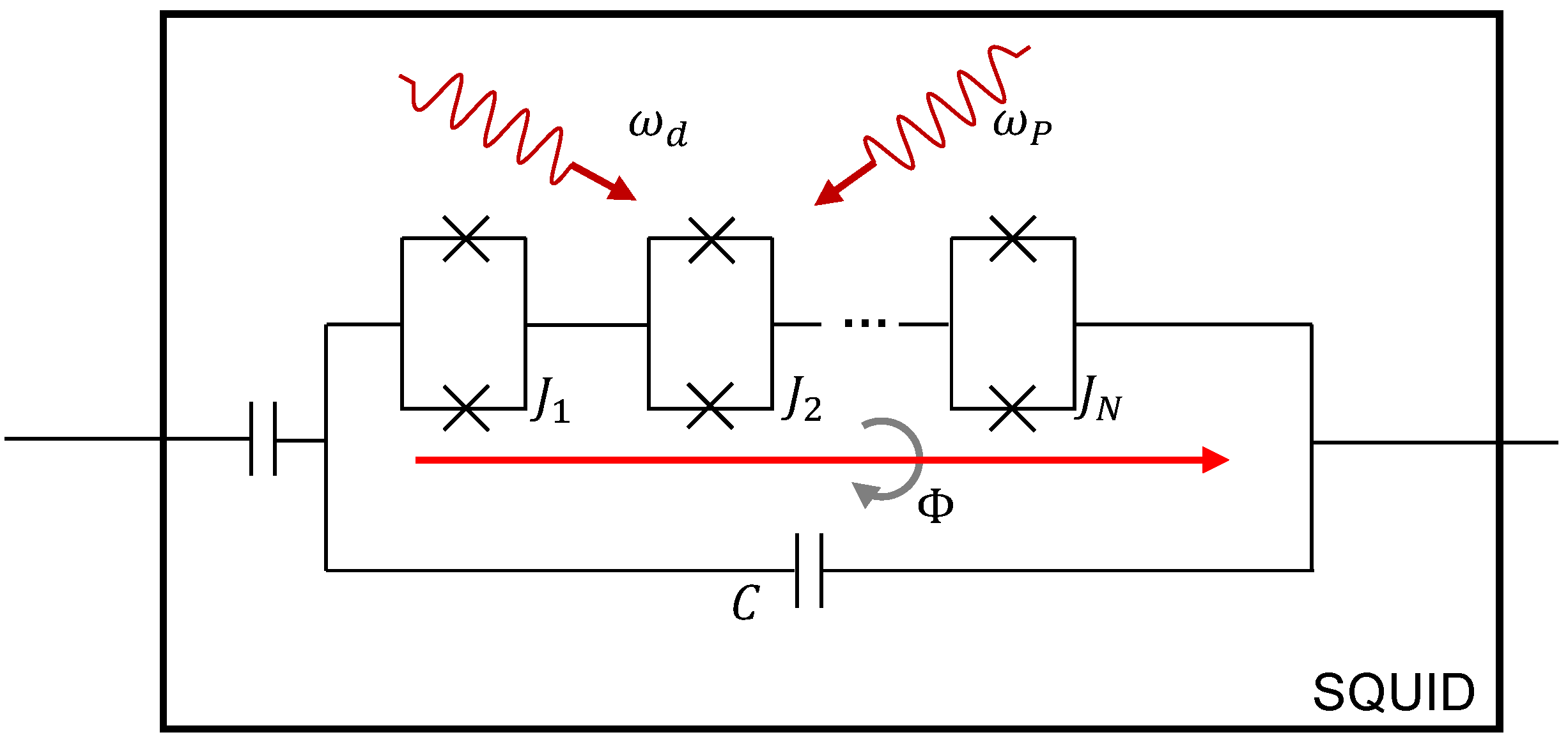
3. The KNPO as the Continuous Variable System

We realize the continuous variable system by considering the model in ref. [47]. This model consists of a large capacitor and N Josephson junctions, with the use of the high-frequency magnetic flux to construct the SQUID array.

As shown in Figure 2, the corresponding Hamiltonian is ($\hslash =1$ is set):

$${\widehat{H}}_{SQUID}=4E_C{\widehat{n}}^2-N{E}_J(\mathsf{\Phi }(t))cos\frac{\widehat{\varphi }}{N},$$

(4)

where $\widehat{n}$ is the number of Cooper pairs and $\widehat{\varphi }$ is the phase over the Josephson junctions array, $E_C$ is the charging energy including shunt capacitor and parasitic capacitance of Josephson junctions and $E_J$ is the Josephson energy for the SQUID array controlled by the external flux $\mathsf{\Phi }(t)$. This flux is harmonically modulated around its mean value with a small amplitude, so $E_J(\mathsf{\Phi }(t))$ can be approximated as $E_J+\delta E_{J}cos{\omega }_{m}t$, where ${\omega }_m$ is the harmonic frequency. Since $\widehat{\varphi }$ is a small quantity (see Appendix B), we can make the Taylor expansion to the second term and drop the high-order terms. Due to the commutation relation $[\widehat{\varphi },\widehat{n}]=i\hslash$, we can rewrite this Hamiltonian using bosonic operators $\widehat{a}$ and ${\widehat{a}}^{†}$:

$${\widehat{H}}_{bosonic}={\omega }_c{\widehat{a}}^{†}\widehat{a}+\frac{K}{6}{(\widehat{a}+{\widehat{a}}^{†})}^4-[2P{(\widehat{a}+{\widehat{a}}^{†})}^2+\frac{4KP}{3{\omega }_c}{(\widehat{a}+{\widehat{a}}^{†})}^4]cos{\omega }_{m}t,$$

(5)

where $\widehat{n}$ and $\widehat{\varphi }$ are expressed by the bosonic operators $\widehat{a}$ and ${\widehat{a}}^{†}$: $\widehat{n}={(\frac{E_J}{32N{E}_C})}^{\frac{1}{4}}i({\widehat{a}}^{†}-\widehat{a})$ and $\widehat{\varphi }={(\frac{2N{E}_C}{E_J})}^{\frac{1}{4}}({\widehat{a}}^{†}+\widehat{a})$, ${\omega }_c=\sqrt{8E_C{E}_J/N}$, $K=-E_C/2N^2$ and $P=-{\omega }_c\delta E_J/8E_J$. Here, K and P correspond to the Kerr-nonlinearity and the pump strength of the KNPO, respectively. We control $4KP\ll 3{\omega }_c$ to drop the last term, turn into the rotating frame at the frequency ${\omega }_m/2$, and drop the high-frequency terms according to the rotating wave approximation. The effective Hamiltonian is:

$${\widehat{H}}_{eff}=K{\widehat{a}}^{†2}{\widehat{a}}^2+\Delta {\widehat{a}}^{†}\widehat{a}-P({\widehat{a}}^2+{\widehat{a}}^{†2}),$$

(6)

with $\Delta ={\omega }_c+2K-{\omega }_m/2$. The constructed KPNO system dominated by the Hamiltonian (6) possesses two degenerate ground states of the continuous variable kind, i.e., the even and odd Schr$\ddot{o}$dinger cat states:

$$\begin{array}{c}|C^{+}\rangle =N_{+}(|+\alpha \rangle +|-\alpha \rangle ),\\ |C^{-}\rangle =N_{-}(|+\alpha \rangle -|-\alpha \rangle ),\end{array}$$

(7)

where $\alpha =\sqrt{P/K}$ and $N_{\pm }=\frac{1}{{(2\pm 2e^{-{2\left|\alpha \right|}^2})}^{1/2}}$.

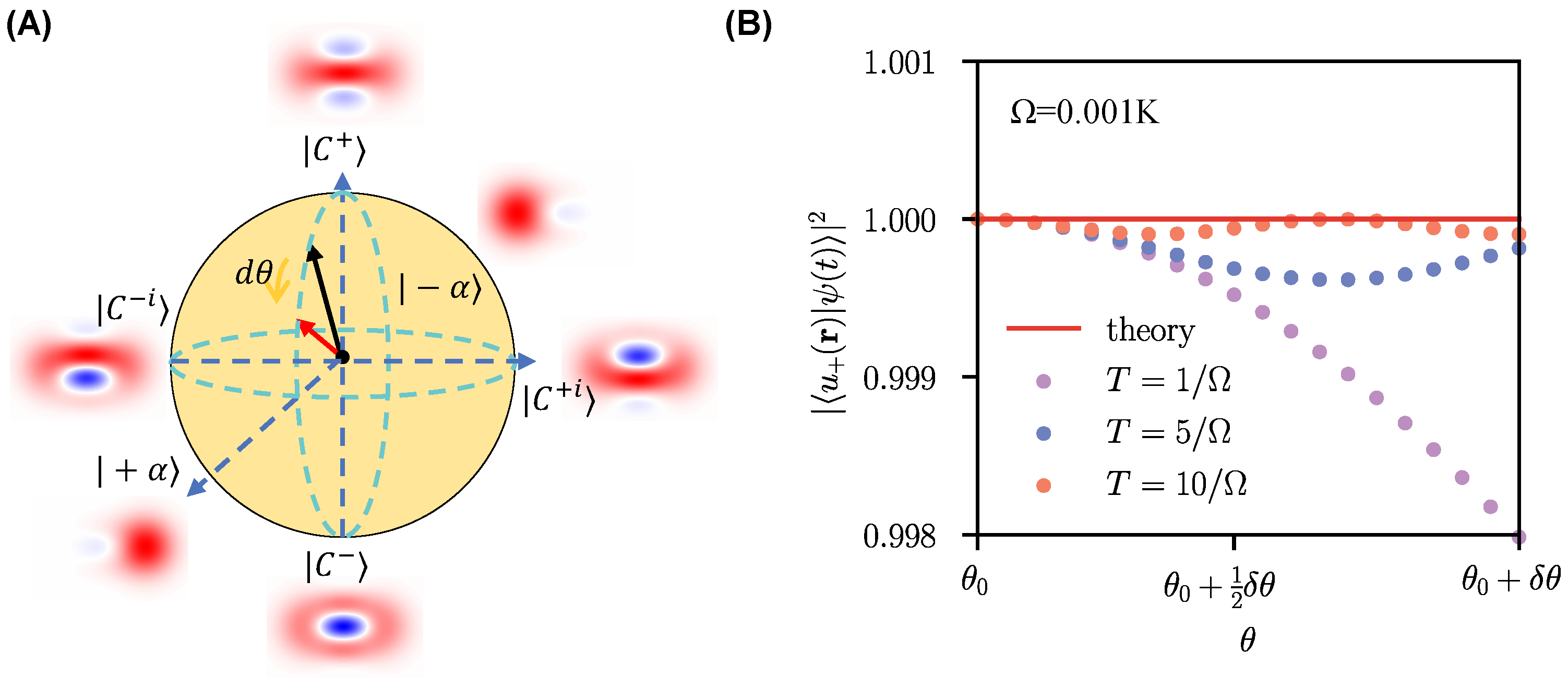
4. Arbitrary Manipulation of the Continuous Variable System

We now turn to the discussion of the arbitrary manipulation of the continuous variable system, with the full Hamiltonian modelled as:

$$\begin{array}{cc}\hfill {\widehat{H}}_{full}=& K{\widehat{a}}^{†2}{\widehat{a}}^2-P({\widehat{a}}^2+{\widehat{a}}^{†2})+\Delta {\widehat{a}}^{†}\widehat{a}+{\widehat{H}}_d,\\ \hfill {\widehat{H}}_d=& 2{ϵ}_{x}cos{\omega }_{d}t({\widehat{a}}^{†}+\widehat{a})+2{ϵ}_{y}cos{\omega }_{p}t({\widehat{a}}^{†}-\widehat{a}),\end{array}$$

(8)

where ${ϵ}_{x/y}$ and ${\omega }_{d/p}$ are the amplitudes and the angular frequencies of the drives, respectively. We let ${\omega }_d={\omega }_p={\omega }_{shift}$ and rotate into the frame of ${\widehat{H}}_0=\frac{{\omega }_{shift}}{2}{\widehat{a}}^{†}\widehat{a}+K{\widehat{a}}^{†2}{\widehat{a}}^2-P({\widehat{a}}^2+{\widehat{a}}^{†2})$. By neglecting the high-order oscillation terms, we then rewrite the Hamiltonian in the basis of cat states:

$${\widehat{H}}_{two}={\mathsf{\Omega }}_x{\widehat{\tilde{\sigma }}}_x+{\mathsf{\Omega }}_y{\widehat{\tilde{\sigma }}}_y+{\mathsf{\Omega }}_z{\widehat{\tilde{\sigma }}}_z,$$

(9)

with

$$\begin{array}{cc}\hfill {\mathsf{\Omega }}_x=& 4\alpha N_{-}{N}_{+}{ϵ}_x,\\ \hfill {\mathsf{\Omega }}_y=& -4{ϵ}_y\alpha N_{-}{N}_{+}{e}^{-{2\left|\alpha \right|}^2}i,\\ \hfill {\mathsf{\Omega }}_z=& (\Delta -{\omega }_{shift})8{\left|\alpha \right|}^2{N}_{+}^2{N}_{-}^2{e}^{-{2\left|\alpha \right|}^2},\end{array}$$

(10)

where ${\widehat{\tilde{\sigma }}}_i(i\in \{x,y,z\})$ are the Pauli operators defined with the continuous variable state space $\{|C^{+}\rangle ,|C^{-}\rangle \}$. It should be noted that $e^{-{2\left|\alpha \right|}^2}$ is an exponential function about average photon number ${\left|\alpha \right|}^2$ of the cat state component, so the amplitude of coherent state $\left|\alpha \right|$ should be small. What is more, to evade the high-level leakage, we should keep ${\mathsf{\Omega }}_y$ and ${\mathsf{\Omega }}_z$ small. According to the formula of the effective two-level system, we let ${\mathsf{\Omega }}_z=\frac{\mathsf{\Omega }}{2}cos\theta$, ${\mathsf{\Omega }}_x=\frac{\mathsf{\Omega }}{2}sin\theta cos\varphi$, and ${\mathsf{\Omega }}_y=\frac{\mathsf{\Omega }}{2}sin\theta sin\varphi$, with $\theta \in [0,\pi ],\varphi \in [0,2\pi ]$.

To check the stability of this system, we performed the simple numerical simulation, by initialing the system’s state in the ground eigenstate of ${\widehat{H}}_{two}(\theta =\frac{\pi }{4},\varphi =0)$ and adiabatically evolving this system into ${\widehat{H}}_{two}(\theta =\frac{\pi }{4}+d\theta ,\varphi =0)$, where $d\theta =\pi /32$. Note that the numerical calculations are performed through the truncation of the infinite-dimension Fock basis state Hilbert space to the dimension of 20. For the duration with the large enough $T\gg 1/(P^2/K)$, the system with the initial state will adiabatically evolve along $|u^{+}(\mathbf{r})\rangle$ to reach a final state. In Figure 3B, we show the fidelity $|\langle u^{+}(\mathbf{r})|\psi (t)\rangle {|}^2$ as a function of the variable $\theta$ for the set of reasonably chosen parameters, with the numerical results well consistent with the theory for a large enough T. For the cases with the reduced evolution time T, the fidelity is slightly deviated, as also depicted in Figure 3B.

5. Method for the Measurement of the QMT

To extract the QMT, we use the definition of quantum distance (see Appendix C of ref. [39]). First, we make a single-parametric modulation to the Hamiltonian $\widehat{H}(\mathbf{r}+\frac{t}{T}\delta r_i{\mathbf{e}}_i)$ and set the initial state the eigenstate state of the initial Hamiltonian $\widehat{H}(\mathbf{r})$ with quantum number k. After the adiabatic evolution with the period T, we measure the excited probability $P_{ii}^k=1-{|\langle u_k(\mathbf{r}+\frac{t}{T}\delta r_i{\mathbf{e}}_i)|\psi (t)\rangle |}^2$, which can be achieved by mapping the continuous variable basis state to the Fock qubit and followed by dispersive readout [50]. According to the Equation (3), we can obtain the diagonal elements of the QMT:

$$g_{ii}^k=\frac{P_{ii}^k}{d{r}_i^2}.$$

(11)

We then make two-parametric modulation $\widehat{H}(\mathbf{r}+\frac{t}{T}\delta r_i{\mathbf{e}}_i+\frac{t}{T}\delta r_j{\mathbf{e}}_j)$ and $\widehat{H}(\mathbf{r}+\frac{t}{T}\delta r_i{\mathbf{e}}_i-\frac{t}{T}\delta r_j{\mathbf{e}}_j)$ to measure the corresponding probability $P_{ij}^{k+}=g_{ii}^{k}d{r}_i^2+2g_{ij}^{k}d{r}_{i}d{r}_j+g_{jj}^{k}d{r}_j^2$ and $P_{ij}^{k-}=g_{ii}^{k}d{r}_i^2-2g_{ij}^{k}d{r}_{i}d{r}_j+g_{jj}^{k}d{r}_j^2$. These two probabilities can be exploited to calculate the off-diagonal elements of the QMT:

$$g_{ij}^k=\frac{P_{ij}^{k+}-P_{ij}^{k-}}{4d{r}_{i}d{r}_j}.$$

(12)

Numerical simulations are performed to verify this theory. Note that, for the numerical calculations, the infinite-dimension Fock basis state Hilbert space is truncated to the dimension of 20, for the set of reasonably chosen parameters. We consider the effective two-level Hamiltonian:

$$\widehat{H}(\theta ,\varphi )=\frac{\mathsf{\Omega }}{2}\left(\begin{array}{cc}cos\theta & sin\theta e^{-i\varphi }\\ sin\theta e^{i\varphi }& -cos\theta \end{array}\right),$$

(13)

which can be constructed in Equation (9), with the effective ground state $|u_{-}\rangle =sin\frac{\theta }{2}|C^{+}\rangle -cos\frac{\theta }{2}{e}^{i\varphi }|C^{-}\rangle$ and the effective excited state $|u_{+}\rangle =cos\frac{\theta }{2}|C^{+}\rangle +sin\frac{\theta }{2}{e}^{i\varphi }|C^{-}\rangle$. By substituting them into Equation (2), we get the QMT:

$$g_{\pm }=\mathrm{Re}\{Q\}=\left(\begin{array}{cc}\frac{1}{4}& 0\\ 0& \frac{1}{4}{sin}^2\theta \end{array}\right).$$

(14)

Here, we initialize the quantum state in the ground state of the Hamiltonian $\widehat{H}({\theta }_0,{\varphi }_0)$, perform two single-parametric modulations $\widehat{H}({\theta }_0+\frac{t}{T}\delta \theta ,{\varphi }_0)$ and $\widehat{H}({\theta }_0,{\varphi }_0+\frac{t}{T}\delta \varphi )$ to calculate the diagonal elements of the QMT, and two two-parametric modulations $\widehat{H}({\theta }_0+\frac{t}{T}\delta \theta ,{\varphi }_0+\frac{t}{T}\delta \varphi )$ and $\widehat{H}({\theta }_0+\frac{t}{T}\delta \theta ,{\varphi }_0-\frac{t}{T}\delta \varphi )$ to calculate the off-diagonal elements of the QMT.

The numerical results are shown in Figure 4, which displays the elements of the QMT as the function of the initial condition ${\theta }_0$ (here we set ${\varphi }_0=0$), showing the accordance between the theoretical (solid lines) and numerical (dots) results.

6. Discussion and Conclusions

In summary, we have proposed a new scheme for the measurement of the QMT with a modulated KNPO system, achieved first by the adiabatic manipulation of the KNPO within the parametric space defined with the continuous variable Schr$\ddot{o}$dinger even and odd cat state bases, and followed by the acquirement of the excited probabilities. The numerical calculations were performed by the adoption of the continuous variable system states defined in the truncated indefinite-dimensional Fock state Hilbert space, and by use of the reasonably chosen parameters.

The measurement of the QMT based on the modulated KNPO system can be, in principle, achieved by use of a microwave-driving superconducting nonlinear inductive element [50]. As compared with the previously demonstrated methods that adopt the discrete two-level solid-state systems [39,40,41], our method provides an alternative for the exploration of geometry and its relevant topology with quantum physical systems, and can be extended to reveal the geometry and topology with interacting [40,41] or high-dimensional [53,54] continuous variable systems.

References

1. Kibble, T.W.B. Geometrization of quantum mechanics. Commun. Math. Phys. 1979, 65, 189–201. [Google Scholar] [CrossRef]
2. Anandan, J.; Aharonov, Y. Geometry of quantum evolution. Phys. Rev. Lett. 1990, 65, 1697–1700. [Google Scholar] [CrossRef] [PubMed]
3. Brody, D.C.; Hughston, L.P. Geometric quantum mechanics. J. Geom. Phys. 2001, 38, 19–53. [Google Scholar] [CrossRef] [Green Version]
4. Kolodrubetz, M.; Sels, D.; Mehta, P.; Polkovnikov, A. Geometry and non-adiabatic response in quantum and classical systems. Phys. Rep. 2017, 697, 1–87. [Google Scholar] [CrossRef] [Green Version]
5. Campos Venuti, L.; Zanardi, P. Quantum Critical Scaling of the Geometric Tensors. Phys. Rev. Lett. 2007, 99, 095701. [Google Scholar] [CrossRef] [Green Version]
6. Ma, Y.Q.; Chen, S.; Fan, H.; Liu, W.M. Abelian and non-Abelian quantum geometric tensor. Phys. Rev. B 2010, 81, 245129. [Google Scholar] [CrossRef] [Green Version]
7. Cheng, R. Quantum Geometric Tensor (Fubini-Study Metric) in Simple Quantum system. arXiv 2013, arXiv:1502.03551. [Google Scholar]
8. Provost, J.P.; Vallee, G. Riemannian structure on manifolds of quantum states. Commun. Math. Phys. 1980, 76, 289–301. [Google Scholar] [CrossRef]
9. Aharonov, Y.; Bohm, D. Significance of Electromagnetic Potentials in the Quantum Theory. Phys. Rev. 1959, 115, 485–491. [Google Scholar] [CrossRef] [Green Version]
10. Xiao, D.; Chang, M.C.; Niu, Q. Berry phase effects on electronic properties. Rev. Mod. Phys. 2010, 82, 1959–2007. [Google Scholar] [CrossRef] [Green Version]
11. Bohm, A.R.; Mostafazadeh, A.; Koizumi, H.; Niu, Q.; Zwanziger, J. The Geometric Phase in Quantum Systems: Foundations, Mathematical Concepts, and Applications in Molecular and Condensed Matter Physics; Springer: Berlin/Heidelberg, Germany, 2003. [Google Scholar]
12. Pachos, J.; Zanardi, P.; Rasetti, M. Non-Abelian Berry connections for quantum computation. Phys. Rev. A 1999, 61, 010305. [Google Scholar] [CrossRef] [Green Version]
13. Zanardi, P.; Rasetti, M. Holonomic quantum computation. Phys. Lett. A 1999, 264, 94–99. [Google Scholar] [CrossRef] [Green Version]
14. Berry, M.V. Quantal phase factors accompanying adiabatic changes. Proc. R. Soc. Lond. A Math. Phys. Sci. 1984, 392, 45–57. [Google Scholar] [CrossRef]
15. Hasan, M.Z.; Kane, C.L. Colloquium: Topological insulators. Rev. Mod. Phys. 2010, 82, 3045–3067. [Google Scholar] [CrossRef] [Green Version]
16. Wen, X.G. Mean-field theory of spin-liquid states with finite energy gap and topological orders. Phys. Rev. B 1991, 44, 2664–2672. [Google Scholar] [CrossRef] [Green Version]
17. Wen, X.G. Colloquium: Zoo of quantum-topological phases of matter. Rev. Mod. Phys. 2017, 89, 041004. [Google Scholar] [CrossRef] [Green Version]
18. Zhang, D.W.; Zhu, Y.Q.; Zhao, Y.X.; Yan, H.; Zhu, S.L. Topological quantum matter with cold atoms. Adv. Phys. 2018, 67, 253–402. [Google Scholar] [CrossRef]
19. Qi, X.L.; Zhang, S.C. Topological insulators and superconductors. Rev. Mod. Phys. 2011, 83, 1057–1110. [Google Scholar] [CrossRef] [Green Version]
20. Armitage, N.; Mele, E.; Vishwanath, A. Weyl and Dirac semimetals in three-dimensional solids. Rev. Mod. Phys. 2018, 90, 015001. [Google Scholar] [CrossRef] [Green Version]
21. Wootters, W.K. Statistical distance and Hilbert space. Phys. Rev. D 1981, 23, 357–362. [Google Scholar] [CrossRef]
22. Braunstein, S.L.; Caves, C.M. Statistical distance and the geometry of quantum states. Phys. Rev. Lett. 1994, 72, 3439–3443. [Google Scholar] [CrossRef]
23. Souza, I.; Wilkens, T.; Martin, R.M. Polarization and localization in insulators: Generating function approach. Phys. Rev. B 2000, 62, 1666–1683. [Google Scholar] [CrossRef] [Green Version]
24. Ozawa, T.; Goldman, N. Probing localization and quantum geometry by spectroscopy. Phys. Rev. Res. 2019, 1, 032019. [Google Scholar] [CrossRef] [Green Version]
25. Roy, R. Band geometry of fractional topological insulators. Phys. Rev. B 2014, 90, 165139. [Google Scholar] [CrossRef] [Green Version]
26. Lim, L.K.; Fuchs, J.N.; Montambaux, G. Geometry of Bloch states probed by Stückelberg interferometry. Phys. Rev. A 2015, 92, 063627. [Google Scholar] [CrossRef] [Green Version]
27. Palumbo, G.; Goldman, N. Revealing Tensor Monopoles through Quantum-Metric Measurements. Phys. Rev. Lett. 2018, 121, 170401. [Google Scholar] [CrossRef] [Green Version]
28. Zanardi, P.; Paunković, N. Ground state overlap and quantum phase transitions. Phys. Rev. E 2006, 74, 031123. [Google Scholar] [CrossRef] [Green Version]
29. Carollo, A.; Valenti, D.; Spagnolo, B. Geometry of quantum phase transitions. Phys. Rep. 2020, 838, 1–72. [Google Scholar] [CrossRef] [Green Version]
30. Zanardi, P.; Giorda, P.; Cozzini, M. Information-Theoretic Differential Geometry of Quantum Phase Transitions. Phys. Rev. Lett. 2007, 99, 100603. [Google Scholar] [CrossRef]
31. Rezakhani, A.T.; Abasto, D.F.; Lidar, D.A.; Zanardi, P. Intrinsic geometry of quantum adiabatic evolution and quantum phase transitions. Phys. Rev. A 2010, 82, 012321. [Google Scholar] [CrossRef] [Green Version]
32. Ma, Y.Q.; Gu, S.J.; Chen, S.; Fan, H.; Liu, W.M. The Euler number of Bloch states manifold and the quantum phases in gapped fermionic systems. Europhys. Lett. 2013, 103, 10008. [Google Scholar] [CrossRef] [Green Version]
33. Kolodrubetz, M.; Gritsev, V.; Polkovnikov, A. Classifying and measuring geometry of a quantum ground state manifold. Phys. Rev. B 2013, 88, 064304. [Google Scholar] [CrossRef] [Green Version]
34. Neupert, T.; Chamon, C.; Mudry, C. Measuring the quantum geometry of Bloch bands with current noise. Phys. Rev. B 2013, 87, 245103. [Google Scholar] [CrossRef] [Green Version]
35. Ozawa, T. Steady-state Hall response and quantum geometry of driven-dissipative lattices. Phys. Rev. B 2018, 97, 041108. [Google Scholar] [CrossRef] [Green Version]
36. Bleu, O.; Malpuech, G.; Gao, Y.; Solnyshkov, D. Effective Theory of Nonadiabatic Quantum Evolution Based on the Quantum Geometric Tensor. Phys. Rev. Lett. 2018, 121, 020401. [Google Scholar] [CrossRef] [PubMed] [Green Version]
37. Bleu, O.; Solnyshkov, D.D.; Malpuech, G. Measuring the quantum geometric tensor in two-dimensional photonic and exciton-polariton systems. Phys. Rev. B 2018, 97, 195422. [Google Scholar] [CrossRef] [Green Version]
38. Klees, R.; Rastelli, G.; Cuevas, J.; Belzig, W. Microwave Spectroscopy Reveals the Quantum Geometric Tensor of Topological Josephson Matter. Phys. Rev. Lett. 2020, 124, 197002. [Google Scholar] [CrossRef]
39. Tan, X.; Zhang, D.W.; Yang, Z.; Chu, J.; Zhu, Y.Q.; Li, D.; Yang, X.; Song, S.; Han, Z.; Li, Z.; et al. Experimental Measurement of the Quantum Metric Tensor and Related Topological Phase Transition with a Superconducting Qubit. Phys. Rev. Lett. 2019, 122, 210401. [Google Scholar] [CrossRef] [PubMed] [Green Version]
40. Zheng, W.; Xu, J.; Ma, Z.; Li, Y.; Dong, Y.; Zhang, Y.; Wang, X.; Sun, G.; Wu, P.; Zhao, J.; et al. Measuring Quantum Geometric Tensor of Non-Abelian System in Superconducting Circuits. Chin. Phys. Lett. 2022, 39, 100202. [Google Scholar] [CrossRef]
41. Yu, M.; Yang, P.; Gong, M.; Cao, Q.; Lu, Q.; Liu, H.; Zhang, S.; Plenio, M.B.; Jelezko, F.; Ozawa, T.; et al. Experimental measurement of the quantum geometric tensor using coupled qubits in diamond. Natl. Sci. Rev. 2019, 7, 254–260. [Google Scholar] [CrossRef] [PubMed] [Green Version]
42. Chamberland, C.; Noh, K.; Arrangoiz-Arriola, P.; Campbell, E.T.; Hann, C.T.; Iverson, J.; Putterman, H.; Bohdanowicz, T.C.; Flammia, S.T.; Keller, A.; et al. Building a Fault-Tolerant Quantum Computer Using Concatenated Cat Codes. PRX Quantum 2022, 3, 010329. [Google Scholar] [CrossRef]
43. Mirrahimi, M.; Leghtas, Z.; Albert, V.V.; Touzard, S.; Schoelkopf, R.J.; Jiang, L.; Devoret, M.H. Dynamically protected cat-qubits: A new paradigm for universal quantum computation. New J. Phys. 2014, 16, 045014. [Google Scholar] [CrossRef]
44. Nigg, S.E. Deterministic Hadamard gate for microwave cat-state qubits in circuit QED. Phys. Rev. A 2014, 89, 022340. [Google Scholar] [CrossRef] [Green Version]
45. Yi, X.; Yang, Q.F.; Zhang, X.; Yang, K.Y.; Li, X.; Vahala, K. Single-mode dispersive waves and soliton microcomb dynamics. Nat. Commun. 2017, 8, 14869. [Google Scholar] [CrossRef] [Green Version]
46. Yang, C.P.; Su, Q.P.; Zheng, S.B.; Nori, F.; Han, S. Entangling two oscillators with arbitrary asymmetric initial states. Phys. Rev. A 2017, 95, 052341. [Google Scholar] [CrossRef] [Green Version]
47. Wang, Z.; Pechal, M.; Wollack, E.A.; Arrangoiz-Arriola, P.; Gao, M.; Lee, N.R.; Safavi-Naeini, A.H. Quantum Dynamics of a Few-Photon Parametric Oscillator. Phys. Rev. X 2019, 9, 021049. [Google Scholar] [CrossRef] [Green Version]
48. Puri, S.; Boutin, S.; Blais, A. Engineering the quantum states of light in a Kerr-nonlinear resonator by two-photon driving. NPJ Quantum Inf. 2017, 3, 18. [Google Scholar] [CrossRef] [Green Version]
49. Goto, H. Universal quantum computation with a nonlinear oscillator network. Phys. Rev. A 2016, 93, 50301. [Google Scholar] [CrossRef] [Green Version]
50. Grimm, A.; Frattini, N.E.; Puri, S.; Mundhada, S.O.; Touzard, S.; Mirrahimi, M.; Girvin, S.M.; Shankar, S.; Devoret, M.H. Stabilization and operation of a Kerr-cat qubit. Nature 2020, 584, 205–209. [Google Scholar] [CrossRef] [PubMed]
51. Yurke, B.; Stoler, D. The dynamic generation of Schrödinger cats and their detection. Phys. B+C 1988, 151, 298–301. [Google Scholar] [CrossRef]
52. Leghtas, Z.; Touzard, S.; Pop, I.M.; Kou, A.; Vlastakis, B.; Petrenko, A.; Sliwa, K.M.; Narla, A.; Shankar, S.; Hatridge, M.J.; et al. Confining the state of light to a quantum manifold by engineered two-photon loss. Science 2015, 347, 853–857. [Google Scholar] [CrossRef] [PubMed] [Green Version]
53. Sugawa, S.; Salces-Carcoba, F.; Perry, A.R.; Yue, Y.; Spielman, I.B. Second Chern number of a quantum-simulated non-Abelian Yang monopole. Science 2018, 360, 1429–1434. [Google Scholar] [CrossRef] [PubMed] [Green Version]
54. Weber, T.; Fobes, D.M.; Waizner, J.; Steffens, P.; Tucker, G.S.; Böhm, M.; Beddrich, L.; Franz, C.; Gabold, H.; Bewley, R.; et al. Topological magnon band structure of emergent Landau levels in a skyrmion lattice. Science 2022, 375, 1025–1030. [Google Scholar] [CrossRef] [PubMed]
Figure 1. Illustration of the distance between two nearby quantum states in the parametric space. (A) The geometric picture of quantum distance in Brillouin zone T 2 . (B) The geometric picture of quantum distance on Bloch sphere.
Photonics 10 00256 g001
Figure 2. Circuit diagram of the KNPO. The red and gray arrows denote the external flux and the magnetic field, respectively, while two red wave arrows represent the modulated drives.
Photonics 10 00256 g002
Figure 3. The dynamics process of the adiabatic evolution. (A) The Bloch dynamics process of the adiabatic evolution. The Wigner functions of the states at the six cardinal points on the sphere (defined with the cat-qubit) are shown. | C ± = N ± ( | + α ± | α ) , where N ± is normalization factor. Similarly, | C ± i = N ± i ( | + α i | α ) . (B) The fidelities for the numerical and theoretical results, respectively, with θ 0 = π / 4 , ϕ 0 = 0 and δ θ = π / 32 , Ω = 0.001 K , P = K , T = 100 / Ω , r = ( sin θ cos ϕ , sin θ sin ϕ , cos θ ) , | u + ( r ) = cos θ 2 | C + + sin θ 2 e i ϕ | C and | ψ ( t ) is the quantum state in the evolution.
Photonics 10 00256 g003
Figure 4. Extraction of the QMT of the continuous variable system. The numerical results of the QMT g θ θ (yellow dots), g ϕ ϕ (green dots), and g θ ϕ (pink dots) are plotted with the theoretical results (solid lines). The whole adiabatic evolution is simulated with Ω = 0.001 K , P = K , δ θ = δ ϕ = π 32 and T = 100 / Ω .
Photonics 10 00256 g004
Disclaimer/Publisher’s Note: The statements, opinions and data contained in all publications are solely those of the individual author(s) and contributor(s) and not of MDPI and/or the editor(s). MDPI and/or the editor(s) disclaim responsibility for any injury to people or property resulting from any ideas, methods, instructions or products referred to in the content.