1. Introduction
The botanical study of remote sensing at various scales from the molecular to the leaf and canopy levels continues to be of significant interest for monitoring Earth’s resources, detecting forage and grain production, and detecting ecosystem health with human activities. Among all methods [
1], polarized electromagnetic radiation has to date gained special importance [
1]. In this paper, we assess the internal optical properties of leaves with polarimetric measurement with anticipated use at the canopy level. It is important to note that, at both levels, there is still a significant lack experimental observations, particularly those interpreting Muller matrices.
The application of polarimetric methods to the study of botanical samples has a rather extensive history (see, for example, [
2,
3,
4,
5,
6]). To date, a number of very interesting results have been obtained in this context but primarily limited to the use of the degree of polarization (
DoP) of light reflected by plants [
7,
8,
9,
10]. The summary from past work is that the
DoP for botanical samples depends on the state of polarization of the incident light. This is a very important result, since it indicates that the depolarization properties of a plant leaf are anisotropic. Undoubtedly, the
DoP remains an extremely important metric for assessing the subtle features of depolarization of the sample under study. Therefore, in this paper, considerable attention is given to this metric. The literature also shows that polarized light experiments that generate Mueller matrices are a rich source of information [
11,
12,
13,
14,
15].
In this study, we address the problem of using polarized light to discriminate and characterize the properties of single barley leaves in the general context of electromagnetic scattering and to determine the polarimetric observables (vector or/and matrix) that are most effective for characterizing the interaction of a leaf with incident polarized light.
In our previous paper [
16], we reported the results of the experimental Mueller matrices for three groups of leaf samples from barley varieties (
Hordeum vulgare):
Chlorina mutant,
Chlorina etiolated mutant and
Cesaer varieties. These samples differed in internal leaf structure from genetic mutation and by illumination during growth. The repeatability of the measurement results of Mueller matrix elements for such a complex and highly depolarizing samples was demonstrated. We show that the barley leaves of these three groups can be discriminated both for forward and backward scattering. In both cases, the most informative Mueller matrix elements were identified. It was also shown that at backward scattering, the value of linear dichroism increases with the decreasing observation angle. The choice of an incident wavelength of λ = 632.8 nm was determined based on the spectral features of light absorption by chlorophyll molecules [
1]. In addition, we were interested to see whether the problems posed in the paper could be solved at one wavelength with simpler and more compact polarimeters.
The presentation of this study in the form of two accompanying papers is due to the need to perform the most complete, meaningful and detailed analysis of experimental polarimetric data, i.e., the experimental Mueller matrices of the studied samples, in the context of two main approaches: single-value depolarization metrics (Part I) and various additive and multiplicative decompositions of Mueller matrices (Part II). The latter is of particular interest when depolarization is anisotropic.
A description of the mathematical background of the Mueller matrix measurement, which was carried out in this experiment, the geometry of the experiments, detail description of the samples under study and the results of measuring the Muller matrices can be found in [
16]. For convenience, this information is also provided in
Appendix A.
In
Section 2, we briefly review the Mueller matrix approach and single value depolarization metrics used in this paper to describe the depolarizing properties of the samples under study. The results and discussion of our experiments are given in
Section 3.
Section 4 summarizes the main results of the paper.
2. Mueller Matrix Observables to Characterize Depolarization
A transformation between Stokes vectors before and after the interaction of polarized light with a studied sample is completely described by a
real matrix called the Mueller matrix [
17,
18,
19]. The Mueller matrix, which characterizes depolarization and anisotropy properties of a scattering sample for a given wavelength and geometry, is given by:
where
is the Stokes vector (
means transpose):
Here,
,
are orthogonal components of the electrical vector
of light propagating along the
-axis;
is the degree of polarization, see Equation (4) below;
is a phase shift between
and
; angle brackets
denote time averaging; and
,
are azimuth and ellipticity of light polarization, respectively. The first Stokes parameter,
, is the total intensity of light. The other three parameters having the dimension of intensity describe the light polarization in the vertical/horizontal, ±45°, and left and right circular states.
The matrix of the form
is the Mueller matrix. For a given wavelength of incident light and the geometry of the experiment, the Mueller matrix contains the most complete information about the optical characteristics of the sample and does not depend on the incident and exiting.
Perhaps, the most basic and “oldest” depolarization metrics associated directly with the light scattered by or transmitted in a studied sample is the degree of polarization (
DoP) of output light. The
DoP can be readily calculated from the Stokes vector of scattered or transmitted light (Equation (2)) as a ratio of the intensity of the fully polarized portion to the total intensity [
19]:
Evidently, physical acceptable limits of DoP have been defined as 0 ≤ DoP ≤ 1, where the low and high limits correspond to the cases of fully depolarized and polarized light, respectively.
Note that the incident light in our experiments has DoP = 1. After interaction with the samples , DoP will generally be a function of an azimuth and of ellipticity of the incident polarization. The fact that the Mueller matrix describes depolarization means that for a given Mueller matrix there is no corresponding Jones matrix, even if for all input polarizations of fully polarized light output DoP = 1. Note that for different input polarizations, the output DoP can generally be different. That is, depolarization can be anisotropic.
In this paper, to characterize the depolarizing properties of the samples under study, we use the parameters, so-called single value depolarization metrics, which can be obtained directly from the elements of the Mueller matrix and do not require the involvement of Mueller matrix decompositions and/or any auxiliary matrices associated with the given Mueller matrix. In this context, Equation (4) characterizes the depolarizing properties of the sample under study for a given input polarization. In order to use this metric to completely characterize the depolarizing properties of a sample, it is obviously necessary to consider the Stokes parameters as functions of the elements of the Muller matrix of the given sample.
Another commonly used single-value depolarization metric is the following. If we scan for the whole Poincaré sphere of input Stokes vectors, then the following scalar metric related to
DoP can be introduced [
20] to characterize the depolarizing properties of a sample:
This metric is called the average degree of polarization and has the arithmetic mean of the output
DoP averaged equally over the Poincaré sphere [
19]. The
evidently is in a range of
. The extreme values of
correspond to the case of unpolarized and totally polarized output light, respectively.
Another parameter to characterize the depolarization capability of a sample is the depolarization index
proposed more than thirty years ago by Gil and Bernabeu [
21]:
The depolarization index is bounded according to . The extreme values of correspond to the case of unpolarized and totally polarized output light, respectively. It can be seen that has a structure analogous to that of DoP (Equation (4)). Indeed, the numerator is the square root of the sum of the squares of all the matrix elements except , and the denominator is only . The physical meaning of this metric is that it is the distance from the point that represents a given Mueller matrix to the center of the Poincaré sphere in Mueller hyperspace.
While the DoP characterizes the depolarization of output light, characterizes the overall depolarization capability of a sample.
The so-called
metrics is defined as follows [
22,
23]:
where
is the diattenuation parameter and
.
The metric is bounded according to . Specifically, corresponds to a totally depolarizing sample; describes a partially depolarizing sample; represents a partially depolarizing sample if otherwise, it represents a non-depolarizing diattenuating sample; finally, for a non-depolarizing non-diattenuating sample.
It can be seen that the metric
, representing the relationship between diattenuation
and depolarization, significantly expands the classification of the studied samples compared to
and
based on polarized light. As a logical supplement to
-metric, in [
24], metric
, which determines the relationship between polarization (i.e., the inclusion into consideration of the matrix elements
,
, and
that describe the ability of the sample under study to polarize the input unpolarized light) and depolarization was proposed. This made it possible to add an additional category of partially polarizing samples to the classification, which is determined by the metric
.
The metric
is defined as:
where
Note that the matrices and , being useful for the definition of on a simple manner, are not Mueller matrices.
Metric gives the following classification of the samples: (i) a totally depolarizing optical system where ; (ii) a partially depolarizing optical system where or if ; (iii) a partially polarizing optical system where if ; (iv) a totally polarizing optical system where if ; and (v) corresponds to the non-depolarizing non-polarizing optical system.
As it can be seen, the depolarization metrics, with the exception of DoP, provide a summary of the depolarizing property of a sample via a single number that varies from zero, thereby corresponding to a totally depolarized output light, to a certain positive number (usually up to 1, and possibly 3 in case of and/or metrics) corresponding to a totally polarized output light. All intermediate values are associated with output partial polarization. Note, that the depolarization metrics DoP (Equation (4)) and (Equation (5)) involve input polarizations, whereas the depolarization index (Equation (6)), -metrics (Equation (7)) and -metrics (Equation (8)) involve the Mueller matrix elements only and need no scanning of the whole Poincaré sphere of input polarizations.
3. Results and Discussion
The measurement strategies we used in the paper are described in [
16] and in the
Appendix A of this paper. All figures throughout of the paper show the dependencies of the depolarization metrics described in
Section 2 on the observation angle for forward and backward scattering. Therefore, to designate the samples under study, a uniform legend is used throughout the text below:
- (a)
Solid square—Chlorina mutant, which was grown under ordinary lighting conditions;
- (b)
Open square—Chlorina mutant, whose plants were etiolated from being left in the dark during growth;
- (c)
Solid triangle—Cesaer varieties.
In order not to overwhelm the figures, we did not label the abscissa axis every time. The ordinate axes are properly indicated in every case throughout the text.
All figures in the text below do not have error bars because the standard deviations in each case are comparable to the plotted symbols and are less than 2%.
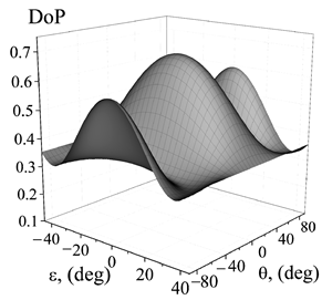
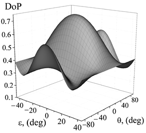
We begin the analysis of the depolarizing properties of the samples under study with very interesting information obtained from the analysis of
DoP (Equation (4)) for some observation angles on input polarizations.
Table 1 represents such dependencies for exact forward scattering (observation angels
) and backward scattering (observation angle
), respectively.
In
Table 2, the minimal and maximal values of output
DoP and corresponding values of azimuth
and ellipticity
of input polarizations for all dependences in
Table 1 are presented.
Obviously, the conclusion following from the dependencies presented in
Table 1 is that all three groups of samples are characterized by pronounced depolarization anisotropy.
The depolarization anisotropy, as can be seen, is quite different for forward and backward scattering for all three groups of samples. For groups of leaves (a) and (b), there is a significant difference in the “sensitivity” of DoP for forward and backward scattering. It can be seen that for backscattering, these two groups of samples are characterized by higher contrast showing the ability to distinguish the sample groups by DoP. For the sample (c) group, we have a somewhat different situation. Namely, the sensitivity of the degree of polarization for forward and backward scattering is approximately the same, although the character of the dependencies is different.
Particular interest for the analysis of the results in
Table 1 presents information on the parameters of the input polarizations at which the minimum and maximum values of the output depolarization are achieved, which are presented in
Table 2. The highest sensitivity is observed for input polarizations close to linear polarization (see
Table 3). Indeed, the modulus of ellipticity does not exceed
degrees, while the azimuths of the input polarizations may differ significantly.
Interestingly, the output
DoP for the input circular polarizations always exceeds the minimum values of
DoP presented in
Table 2. This is especially true for backscattering.
Thus, these dependencies provide very effective grounds for differentiating the samples under study in both forward and backward scattering directions.
Analyzing the explicit form of the experimental Mueller matrices in [
16] (see also
Figure A3), we determined that non-zero values for the matrix elements
and
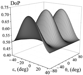
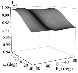
are observed for backscattering. The latter means there is linear dichroism for given observation angles. We next take a look at this effect.
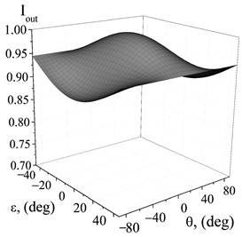
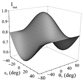
Table 4 shows the dependencies of the output intensity
Iout on the input polarizations for all three groups of leaf samples.
The
Table 5 shows the maximum and minimum output intensity depending on the input polarizations for data presented in
Table 4.
From the presented dependencies (
Table 4 and
Table 5), a more detailed conclusion follows that linear dichroism is generally observed for both forward and back scattering for all three groups of samples. Thus, for all three groups of samples under study for a given observation angle, linear dichroism occurs.
For forward scattering, the effect is much less pronounced than for backscattering. For backscattering, as can be seen, it is quite significant. As expected, the minimum and maximum intensity values are observed at orthogonal input polarizations (see
Table 5). The parameters of dichroism vary for different samples and for different observation angles (see
Table 6). Detailed information about the value, azimuth, and dependence of dichroism on the observation angle will be obtained in the accompanying paper based on the decomposition of the experimental Mueller matrices.
Figure 1a,b present the dependencies of depolarization metrics
(Equation (6)),
(Equation (7)), and
(Equation (5)) on observation angle for forward and backward scattering, respectively.
Based on the behavior of these depolarization metrics, it can be seen that all three groups of barley leaf samples are partial depolarizers. In addition, the degree of depolarization significantly depends on the observation angle for forward scattering. Depolarization takes the greatest values at observation angles close to 90 degrees. This result is quite expected, since light travels a longer path through the thickness of the leaf. Note that for forward scattering, all three depolarization metrics behave quite similarly.
For backscattering, depolarization is generally less dependent on the observation angle. In contrast to forward scattering, the dependence of depolarization metrics on the observation angle is different. The samples of group (b) are characterized by the greatest depolarization, and the dependence of depolarization on the observation angle is non-monotonic. There is a range of observation angles (approximately 125 to 140 degrees) for which the samples of group (b) are close to an ideal depolarizer. The minimum depolarization for all backscattering observation angles is a characteristic for samples of group (c).
In forward scattering, the given metrics make it possible to reliably distinguish between samples of group (b) and pairs (a) and (c). Samples (a) and (c) differ slightly. As for backscattering, the situation is completely different. In almost the entire range of observation angles, all three groups of samples are reliably distinguishable with high contrast. The exception is the angles of 95–125 degrees, for which there is again a convergence of results for groups (a) and (c), although the difference between them is greater than for forward scattering. The -metric shows the greatest potential for distinguishing all three groups of samples. Thus, the illumination mode during plant growth has the greatest influence on the depolarizing properties of the samples under study.
For completeness of analysis,
Figure 2 presents the dependencies of depolarization metric
(Equation (8)) on observation angle for forward and backward scattering, respectively.
Comparing the dependences for depolarization metrics
and
, one can see that they are very similar. That is, the metric
does not carry additional information about the depolarizing properties of the studied groups of samples in comparison with the metric
. Based on both metrics, the samples under study are partially depolarizing objects. This is apparently explained by the fact that for the samples under study, we have
(see
Figure A2 and
Figure A3).
Note that the results presented in this section demonstrate that the analysis of DoP and depolarization metrics carries significantly different information and naturally complements the characterization of the samples under study, specifically for samples demonstrating anisotropy of depolarization.
4. Conclusions
We have presented the results of analysis of the experimental Mueller matrices for three groups of barley leaves based on the single value depolarization metrics: degree of polarization (DoP), average degree of polarization (), depolarization indices (), and the and metrics. The objective of the paper was to determine whether the groups of barley leaves under consideration could be discriminated on the basis of polarimetric observation. The main conclusion that follows from the results presented above is that depolarization is a very effective observable for reliably discriminating different states of leaves of the same plant with different internal structures achieved either due to mutation or by illumination during growth
Indeed, all depolarization metrics we tested in this paper turned out to be sensitive to the characteristics of the samples, and this sensitivity is very different for forward and backward scattering. From among these metrics, the most effective is the
-metric. In addition, special attention should also be given to the
DoP. Actually, in its ability to discriminate the studied groups of samples, the
DoP is not inferior to the
-metric. At the same time, the
DoP allows one to obtain extremely important and interesting information about the anisotropy of depolarization, which itself, as follows from the
Table 1, is also a powerful observable.
As for the measurement mode, the results presented above allow us to correct the preliminary conclusion about the higher efficiency of forward scattering for the identification problem [
16]. All depolarization metrics showed greater efficiency for backscattering. The latter is an extremely important result, since aerial and satellite remote sensing of plants and vegetation measures backscattering.
The fact that all the results presented in the paper were obtained at one wavelength is also very remarkable, since it allows us to identify the samples under study using simpler and cheaper measuring systems.
Another interesting result is dichroism, which turned out to be observed for all three groups of leaves in forward and backward scattering directions (see
Table 4). In backward scattering, this result is expected due to
(see
Figure A3), whereas dichroism for forward scattering is notable. The higher value of dichroism observed for backscattering makes it a very promising identifier, since light intensity is easily measured.


