Review

The 5P3/2→6PJ(J=1/2,3/2) Electric Dipole Forbidden Transitions in Rubidium

by
Francisco Ponciano-Ojeda
1,
Cristian Mojica-Casique
1,
Santiago Hernández-Gómez
1,
Alberto Del Angel
2,
Lina M. Hoyos-Campo
1,
Jesús Flores-Mijangos
1,
Fernando Ramírez-Martínez
1,*,
Daniel Sahagún Sánchez
2,
Rocío Jáuregui
2 and
José Jiménez-Mier
1,*
1
Instituto de Ciencias Nucleares, UNAM, Ciudad de México 04510, Mexico
2
Instituto de Física, UNAM, Ciudad de México 04510, Mexico
*
Authors to whom correspondence should be addressed.
Photonics 2023, 10(12), 1335; https://doi.org/10.3390/photonics10121335
Submission received: 27 October 2023 / Revised: 23 November 2023 / Accepted: 29 November 2023 / Published: 1 December 2023
(This article belongs to the Special Issue Precision Atomic Spectroscopy)

Abstract

:
This paper presents a general review of the results of the experimental and theoretical work carried out by our research group to study the 5 P 3 / 2 6 P J electric quadrupole transition in atomic rubidium. The experiments were carried out with room-temperature atoms in an absorption cell. A steady-state population of atoms in the 5 P 3 / 2 excited state is produced by a a narrow-bandwidth preparation laser locked to the D2 transition. A second CW laser is used to produce the forbidden transition with resolution of the 6 P J hyperfine states of both rubidium isotopes. The process is detected by recording the 420(422) nm fluorescence that occurs when the atoms in the 6 P J state decay directly into the 5 S ground state. The fluorescence spectra show a strong dependence on the relative polarization directions of the preparation laser and the beam producing the forbidden transition. This dependence is directly related to a strong anisotropy in the populations of the 5 P 3 / 2 intermediate magnetic substates, and also to the electric quadrupole selection rules over magnetic quantum numbers. A calculation based on the rate equations that includes velocity and detuning dependent transition rates is adequate to reproduce these results. The forbidden transition is also shown to be an ideal probe to measure the Autler–Townes splitting generated in the preparation of the 5 P 3 / 2 state. Examples of spectra obtained with cold atoms in a magneto-optical trap (MOT) are also presented. These spectra show the expected Autler–Townes doublet structure with asymmetric line profiles that result as a consequence of the red-detuning of the trapping laser in the MOT.

1. Introduction

Alkali atoms, with a simple electronic structure, are naturally a good testing ground in the experimental and theoretical study of electromagnetic transitions beyond the electric dipole approximation. Examples of experiments to observe such transitions in room-temperature or hot vapors of alkali atoms include the study of s to d excitations [1,2,3], and also of the relatively strong p to p transitions in rubidium [4,5,6,7,8,9]. There are also experiments in which electric dipole forbidden transitions were observed in cold atoms in magneto-optical traps [10,11,12].
The purpose of this article is to present a review of the main results of the experiments and calculations carried out in our research group to study the 5 P 3 / 2 6 P J ( J = 3 / 2 , 1 / 2 ) electric quadrupole transition in atomic rubidium. To observe this transition, one has to have a significant atomic population in the 5 P 3 / 2 initial state, which is itself an excited state. A narrow bandwidth laser is used to prepare this population. A second laser is then tuned to excite the electric quadrupole transition. This forbidden transition was first reported in [5], where it was shown that the hyperfine structure of the 6 P 3 / 2 state could be resolved, and also that optical pumping and selection of velocity effects determined the overall structure of the electric dipole forbidden spectra. A three-step description was also proposed, which takes advantage of the large disparity in intensities between the strong preparation step and the weak electric quadrupole excitation. The second article [6] is a detailed study of the dependence of the electric quadrupole spectra on the relative polarization directions of the laser preparing the 5 P 3 / 2 initial state of the transition, and of the laser producing the forbidden transition. Results for the 5 P 3 / 2 6 P 1 / 2 transition are given in [7]. A complete calculation was then presented in [8] to explain in detail the use of the electric quadrupole transition as a probe of the Autler–Townes effect induced by the strong mixing of states produced by the preparation step. Finally, in [9], a dynamic model that includes velocity-dependent terms in the rate equation approximation is used to reproduce the positions and intensities of the main transitions and also of the satellites that result from selection of velocity effects.
The structure of this review paper is the following: in Section 2 the overall design of the experiments is shown. The experimental setup is presented in Section 3. Details of the three-step description and of the relationship between the polarization directions and the selection rules are described in Section 4. Examples of experimental spectra and their comparison with the results of the model are shown in Section 5. Here, recent results of spectra obtained in a magneto-optical trap serve to compare the use of the electric quadrupole transition as an ideal probe of the Autler–Townes effect. Finally, the overall conclusions are given in Section 6.

2. The 5 P 3 / 2 6 P J ( J = 3 / 2 , 1 / 2 ) Electric Quadrupole Transitions in Rubidium

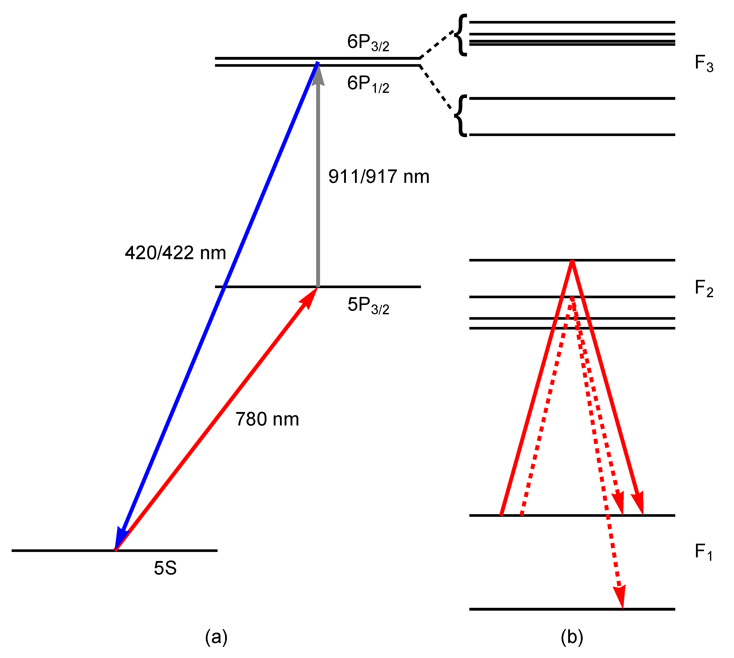
The energy levels relevant to this work are shown in Figure 1. The electric dipole forbidden transition occurs between the 5 P 3 / 2 and the 6 P J ( J = 1 / 2 , 3 / 2 ) fine structure states. The initial state of this transition is also the first excited state of the atom, so it is necessary to excite a significant population of atoms from the ground state into this state. The electric quadrupole transition occurs at 911 nm to excite to the 6 P 3 / 2 state, and at 917 nm if one wants to reach the 6 P 1 / 2 state. Production of the forbidden transition is probed by the detection of the 420(422) nm photons that result from the direct electric dipole decay of the 6 P 3 / 2 ( 1 / 2 ) state into the ground state.
A three-level atom description of the interaction between the two radiation fields and an atom is used as the starting point of the calculations [5,6]. This model considers that the coupling between the 5 P and 6 P states by the forbidden transition is very weak. Therefore, the intensity of the preparation stage will determine the regime that must be used in the calculation. For low intensities the three-level system predicts single decay lines for each F 3 hyperfine state, while for stronger coupling, the Autler–Townes effect takes place [13], and the fluorescence lines split into doublets.
The bandwidths of the lasers used are narrow enough to allow resolution of the hyperfine structure of all three 5 S , 5 P 3 / 2 and 6 P J fine structure states. Therefore, in Figure 1b their hyperfine structure is presented. For the experiments with room-temperature atoms [5,6,7,8,9], the preparation laser selects the value of the total angular momentum F 1 of the ground state. The hyperfine structure and the selection rules for electric dipole transitions determine the characteristics of the 5 S 5 P 3 / 2 preparation step. In particular, important optical pumping effects, combined with the selection of velocities present in the interaction with room-temperature atoms, determine the 5 P 3 / 2 hyperfine states that are significantly populated, and thus determine the structure of the electric quadrupole transition spectra. A distinction must be made in the preparation step between the cyclic transition (indicated by a continuous arrow), and the other non-cyclic transitions (an example shown by the dashed arrows). In the cyclic transition decay occurs only into the same hyperfine ground state; while in the non-cyclic transitions, decay to the other ground hyperfine (dark) state also occurs. Therefore, with the cyclic transition, optical pumping redistributes populations among the different magnetic sublevels, while for non-cyclic transitions, optical pumping effects effectively remove atoms from the preparation step.

3. Experimental Setup

Details of the experimental setup used in this work are given in [5,6,7,8]. For completeness, it is shown schematically in Figure 2.
An external cavity diode laser at 780 nm produces the 5 S 5 P 3 / 2 preparation transition. For most of the experiments, its frequency was locked to the F 1 = I + 1 / 2 F 2 = I + 3 / 2 cyclic transition for zero-velocity atoms. Its linear polarization sets the direction of the quantization (z)-axis, and its propagation direction is then taken as the x-axis. For the 5 P 3 / 2 6 P 3 / 2 experiments, a beam from a 911 nm external cavity laser is sent to the cell in a counter-propagating configuration. Its frequency is scanned across the region that produces electric quadrupole transitions to the different 6 P 3 / 2 hyperfine states. For the 5 P 3 / 2 6 P 1 / 2 experiments, the external cavity diode laser is replaced by a TiSa laser that emits at 917 nm. A half-wave plate is used to set the direction of linear polarization of either of these lasers, relative to that of the 780 nm laser. The 420(422) nm fluorescence that results from the 6 P 3 / 2 ( 1 / 2 ) 5 S decay was detected with a photomultiplier tube (PMT). The direction of detection of the fluorescence photons is perpendicular to both the quantization axis and the laser propagation direction. A lens is used to focus the fluorescence photons into the cathode of the PMT. A bandpass filter centered at 420 nm is placed in the path of the fluorescence photons before they reach the PMT.
The cell used in the experiments was kept at room temperature. Results are also presented of electric quadrupole spectra recorded with cold atoms in a magneto-optical trap (MOT) in continuous operation. The regular six-beam MOT configuration [14] was used. In this case, the trapping and repumping beams are also used for the preparation step. The 911 nm laser is sent to the cold atomic cloud, and the blue fluorescence passes through the bandpass filter and is focused into the PMT cathode. In this case a PMT operating in counting mode was used.
The frequency scale of all experimental spectra presented here was calibrated by directly relating the main peaks to the known hyperfine structure of the 6 P 3 / 2 states in both 85 Rb and 87 Rb [15,16]. We estimate that nonlinearities in the laser frequency scans contribute to uncertainties no greater than 2 MHz in the line positions, and this should have but a minor role in the interpretation of the results. Typical frequency scans took 5 s, and the spectra presented here are the average of tens of such spectra.

4. Theory

4.1. Three-Step Description

The large difference in the coupling intensity of the preparation step with an electric dipole transition and the electric quadrupole excitation, followed by the emission of a blue decay photon, makes it possible to separate the process in three steps to obtain an equation that describes the whole process. The preparation step excites the 5 S 5 P 3 / 2 transition, and therefore it sets the relative populations of the 5 P 3 / 2 F 2 M 2 magnetic sublevels. The electric quadrupole transition then weakly perturbs these populations, producing a small population of atoms in the 6 P 3 / 2 F 3 M 3 states. The fluorescence photons resulting from the direct decay into the 5 S F 1 M 1 ground state are then used to detect the production of the electric quadrupole transition. The probability of detecting this photon from the F 3 state can be written as [5,6,7]
I ( F 3 ) F 1 , M 1 , M 2 , M 3 , λ σ ( F 2 , M 2 ) | F 2 M 2 | T q | F 3 M 3 | 2 | F 3 M 3 | D λ | F 1 M 1 | 2 .
Here, the sum is over all the magnetic projections of the F 2 and F 3 hyperfine states, over all the values of F 1 M 1 allowed by an electric dipole decay and over two polarization directions λ perpendicular to the direction of observation. The first term σ ( F 2 , M 2 ) represents the population of the F 2 M 2 magnetic sublevel that is determined in the preparation step. The second factor then is the square of the electric quadrupole transition matrix element. Finally, the last factor gives the probability of decay into the 5 S F 1 M 1 ground state. It is convenient to analyze each term separately [6].

4.2. Calculation of the σ ( F 2 , M 2 ) Relative Populations

In an absorption cell, a single linearly polarized beam produces the strong preparation transition. In the vast majority of the experiments presented here, its frequency is locked to the F 1 = I + 1 / 2 F 2 = I + 3 / 2 cyclic transition for zero-velocity atoms. Because of its cyclic nature, the atoms decay back to the same F 1 active ground state. One would expect a steady-state population of these F 2 hyperfine states. Therefore, excitation of the electric quadrupole transition from this state should give rise to the dominant fluorescence lines. However, in a room-temperature sample, this laser can also excite atoms with specific velocity projections to the other two F 2 = I + 1 / 2 and F 2 = I 1 / 2 hyperfine states. These states can also decay to the other 5 S hyperfine state. Once they are in this dark state, these atoms no longer participate in the preparation cycle. Therefore, one would expect a smaller population of these two F 2 hyperfine states. The fluorescence peaks observed from the decay of these velocity-selective states are what will referred to as the satellite lines. Furthermore, the relative populations of these two states, compared to the population of the dominant state produced by the cyclic transition, should decrease with an increase in the preparation laser intensity.
The populations of the magnetic sublevels of the three F 2 hyperfine states are obtained by solving the rate equations in the steady state approximation [9]. The terms required for the spectral energy density between states 5 S F 1 and 5 P 3 / 2 F 2 are expressed as the product of the laser light intensity times a Lorentzian line function [17]:
ρ ( δ F 1 F 2 , v z ) I r Γ 5 P 3 / 2 1 1 + 16 π 2 Γ 5 P 3 / 2 2 δ F 1 F 2 v z λ p 2
where v z is the projection of the atom velocity along the laser beam propagation direction, I r is the ratio of the laser intensity to the D2 saturation intensity in rubidium, δ F 1 F 2 = ν p ( ν F 2 ν F 1 ) is its frequency detuning and λ p = 780.24 nm is its wavelength. In this expression, Γ 5 P 3 / 2 = 2 π × 6 MHz is the spontaneous decay rate of the 5 P 3 / 2 state. As a result, one obtains the 5 S and 5 P 3 / 2 populations as functions of the laser detuning and the atom velocity.

4.3. The Electric Quadrupole Transition

Once the σ ( F 2 , M 2 ) relative populations are known, the second term in Equation (1) needs to be evaluated. For a single, linearly polarized laser beam that drives the 5 P 3 / 2 6 P J transition, the electric quadrupole operator is proportional to [6];
T q = ( ϵ ^ · r ) ( k · r ) .
One then takes the propagation direction along the x-axis, so that its polarization vector is written as [6] ϵ ^ = cos θ e ^ z + sin θ e ^ y , where θ is the angle between the linear polarization direction of the 911 nm and the quantization axis. In this geometry one has
T q = k ( x z cos θ + x y sin θ ) .
One can then use the Wigner–Eckart theorem to obtain the selection rules over the magnetic quantum numbers of the hyperfine states. The first term x z can be written as a linear combination of the spherical harmonics Y 2 , ± 1 . The second term is expressed in terms of Y 2 , ± 2 . Therefore, electric quadrupole transitions with parallel polarizations obey the selection rule Δ M = ± 1 . If one uses perpendicular polarizations, the selection rules are Δ M = ± 2 .
Equation (3) also indicates that the decay fluorescence intensity has a cos 2 θ dependence. This dependence can be equivalently cast in the form
I ( F 3 ) = I 0 1 + A 0 P 2 ( cos θ )
where P 2 ( cos θ ) is the second-order Legendre polynomial, and the coefficients I 0 and A 0 can be explicitly written in terms of the populations σ ( F 2 , M 2 ) and of the squares of the electric quadrupole transition reduced matrix elements. Therefore, one also needs the squares of the reduced matrix elements that result from the use of the Wigner–Eckart theorem for the electric quadrupole transition. They can be written as [11]
| 5 P 3 / 2 F 2 | | T | | 6 P J F 3 | 2 = 2 F 2 + 1 2 F 3 + 1 3 / 2 F 2 I F 3 J 2 2 | 5 P 3 / 2 | | T | | 6 P j | 2
where I is the nuclear spin, the curly bracket is the Wigner six-j symbol and 5 P 3 / 2 | | T | | 6 P j is the reduced matrix element common to all 5 P 3 / 2 6 P J hyperfine transitions. Values of the product of the first three terms in this expression that cover both rubidium isotopes and all possible values of total angular momenta are presented in Table 1 and Table 2.
One then multiplies this transition by the detuning and velocity-dependent line profile [9]
g ( δ F 2 F 3 , v z ) = 1 1 + 16 π 2 δ F 2 F 3 + v z λ q 2 Γ 6 P 2 .
Here δ F 2 F 3 = ν q ( ν F 3 ν F 2 ) is the laser detuning and λ q = 911 nm and Γ 6 P = 2 π × 1.34 MHz are the natural width of the 6 P state [18]. The plus sign in the velocity term indicates that this laser counterpropagates with respect to the 780 nm preparation laser.

4.4. Decay into the Ground State

The third term in Equation (1) can also be reduced using Wigner–Eckart’s theorem [6]. Taking into account that in the experimental setup, the detection of the fluorescence photons is along the y-axis, the two polarization directions used in its description are e ^ x and e ^ z . It is then straightforward to write the decay transition matrix elements in terms of the product of a geometrical factor times a single 6 P J 5 S reduced matrix element [6].
As a result of the inclusion of the velocity-dependent line profiles in the preparation of the σ ( F 2 , M 2 ) populations and in the electric quadrupole transition, one ends up with a fluorescence emission probability that is also velocity-dependent. To calculate an electric quadrupole spectrum one has to evaluate the integral of the product of this emission probability multiplied by Maxwell’s velocity distribution for a gas sample of room-temperature atoms. Finally, in order to compare with the experimental results, the convolution of the simulated spectra with a Gaussian window whose width was adjusted between 6 and 9 MHz was performed.

4.5. Scalar Beams with Spatial Structure

Now, we want to focus on the case in which the excitation beam associated with the electric quadrupole transition is a scalar beam with spatial structure. In such a case, the electric quadrupole transition operator has to be written in its general form T q = ( R · r ) ( e r · E ( R ) ) , where R denotes the position of the center of mass of the atom with respect to the beam ( r still represents the internal coordinates of the atom), and E ( R ) is the complex electric field of the excitation beam. It is convenient to express the electric quadrupole transition operator in terms of spherical (or irreducible) tensors as follows
T q = p = 2 2 K p ( 2 ) Q p ( 2 )
where K p ( 2 ) and Q p ( 2 ) = e r 2 4 π 5 Y 2 , p are the spherical tensors [19,20] associated with the rank-2 tensors K j k j E k ( R ) and Q j k = e 1 2 ( 3 r j r k δ i j r 2 ) , respectively. In this way, the quadrupole spherical tensor Q p ( 2 ) contains all the information associated with the atom internal degrees of freedom, and the spherical tensor K p ( 2 ) depends only on the atom center of mass and on the spatial structure of the excitation beam. This information is enough to reconstruct the probability to detect a blue photon I ( F 3 ) . The transition matrix elements in Equation (1) are rewritten by decoupling the nuclear and electronic angular momenta to obtain
I ( F 3 , R ) = I 0 p = 2 2 B p K p ( 2 ) ( R ) 2 ,
where I 0 contains the reduced matrix elements common to all 5 P 3 / 2 6 P J and 6 P J 5 S 1 / 2 terms, and B p depends on the geometric part defined in terms of Wigner three-j and six-j symbols. Note that I ( F 3 , R ) depends on the spatial structure of the excitation beam (encoded in K p ( 2 ) ( R ) ). This means that a strong gradient in the excitation beam spatial structure will significantly modify the spectral lines.
In an experiment with a vapor cell at room temperature, as schematized in Figure 2, the collected blue photons come from a finite volume element V . Integrating over this volume allows us to correctly reconstruct the probability of detecting a blue photon with
I ( F 3 ) = I 0 p = 2 2 B p T p ,
where T p ϱ a t V d V R K p ( 2 ) ( R ) 2 and ϱ a t is the atomic density, which is assumed to be constant inside V , where a low-density medium is also assumed such that collisions and re-absorption processes are negligible. Therefore, in this kind of experiment where I ( F 3 ) no longer depends on R , the spatial structure of the excitation beam can still affect the probability of detecting blue photons. In the remainder of this section we show analytic results for the case of a scalar Bessel beam.
The electric field of a scalar Bessel beam of order m is [21]
E ( R ) = E 0 e i k x x ϵ ^ ψ m x ^ 1 2 k k x ψ m 1 e i θ + ψ m + 1 e i θ
where ψ m J m ( k ρ ) e i m ϕ , J m is the Bessel function, ϵ ^ = cos ( θ ) z ^ + sin ( θ ) y ^ is the polarization vector, E 0 is the field amplitude and ρ = y 2 + z 2 is the radial coordinate (note that the generation of an ideal BB would require an infinite amount of energy [22]; here, we assume that the beam has a finite radius ρ B , i.e., the amplitude is zero for ρ > ρ B ) and ϕ = arctan ( z / y ) is the azimuthal coordinate. Note that sometimes the scalar Bessel beams are described by only the first term of Equation (9) (which is a solution of the wave equation but it does not satisfy Maxwell’s equations). Here, we refer to that approximation as paraxial scalar Bessel beam and we reserve the term scalar Bessel beam for the general case.
The generalized tensors T p for the electric field of a scalar Bessel beam of order m can be written (neglecting the terms containing k 4 k x 4 ) as
( 10 a ) T 0 = 3 k 2 k x 2 c m α m cos 2 θ ( 10 b ) T 1 = c m β m cos 2 θ + 1 2 k 2 k x 2 c m α m + cos 2 θ 2 α m β m β m 1 β m + 1 ( 10 c ) T 2 = c m β m sin 2 θ + 1 4 k 2 k x 2 c m β m 1 + β m + 1 + sin 2 θ 6 α m 4 β m
where c m = γ β m + 1 4 k 2 k x 2 β m 1 + β m + 1 , γ ϱ a t E 0 2 is a proportionality constant, and α m and β m are dimensionless variables defined by m and by the excitation beams waists.
Therefore, in the paraxial limit ( k k x ), the generalized tensors T p only depend on the polarization angle θ , and the result for the plane wave approximation is recovered (see Equation (4)). On the other hand, in the non-paraxial limit, Equation (10) demonstrates that the topological charge of the Bessel beam, m, will affect the values of the generalized tensors. In agreement with previous results [23,24], our model predicts that both the polarization angle θ and the orbital angular momentum of the excitation beam will change the intensity of the quadrupole spectral lines.

5. Results and Discussion

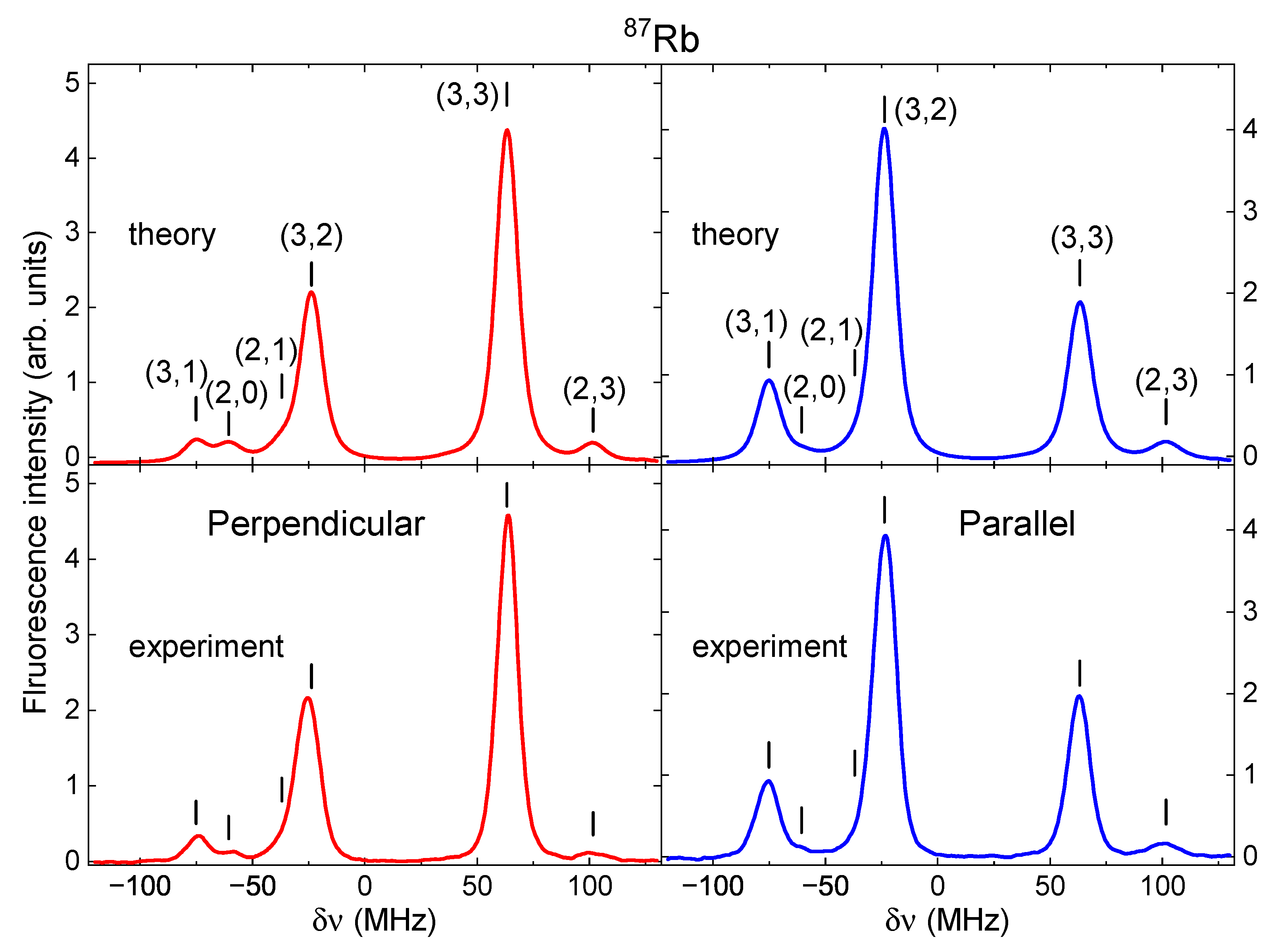
Figure 3 shows an example of fluorescence spectra recorded when the preparation laser is locked to the 5 S F 1 = 2 5 P 3 / 2 F 2 = 3 cyclic transition for atoms with a zero-velocity component. The frequency of the 911 nm laser is scanned across the 5 P 3 / 2 6 P 3 / 2 electric quadrupole transition region. The left-hand panel shows the spectra when the linear polarization of the 911 nm laser is perpendicular to the polarization of the preparation laser. The right-hand panel corresponds to parallel polarizations. The peaks in the spectra are labeled by ( F 2 , F 3 ) , where F 2 is the total angular momentum of the 5 P 3 / 2 initial hyperfine state, and F 3 is the total angular momentum of the 6 P 3 / 2 final state of the electric quadrupole transition. Three peaks are readily identified in both spectra, which result from the excitation of the zero-velocity group of atoms ( F 2 = 3 ) into the 6 P F 3 = 1 , 2 and 3 excited states. However, there are three more peaks that result from excitation of the group of atoms that is prepared in the 5 P 3 / 2 F 2 = 2 state. These correspond to the electric quadrupole transitions F 2 = 2 F 3 = 0 , 1 and 3. Note the absence of the peak corresponding to the F 2 = 2 F 3 = 2 , which is not an allowed electric quadrupole transition. This absence results as a consequence of the null value of the six-j symbol in Table 1. These satellites are clearly present in the spectrum recorded with perpendicular polarizations. For parallel polarizations, only the ( 2 , 3 ) satellite line can be identified. In both spectra the ( 2 , 1 ) transition appears as a shoulder to the low-frequency side of the main ( 3 , 2 ) line. The remarkable differences in the relative intensities of the dominant peaks when the electric quadrupole transition is produced by linearly polarized light with the electric field vector parallel or perpendicular to the quantization axis is a direct manifestation of the selection rules over the magnetic quantum numbers [6]. For parallel polarizations, the electric quadrupole transitions must obey Δ M = ± 1 , while for perpendicular polarization, the selection rule is Δ M = ± 2 . The top panels in Figure 3 show the spectra obtained by solving the set of velocity-dependent rate equations [9]. The excellent agreement between experiment and theory shows that the three-step description accurately reproduces the position, relative intensity and polarization dependence of the main lines and also of the velocity-dependent satellites.
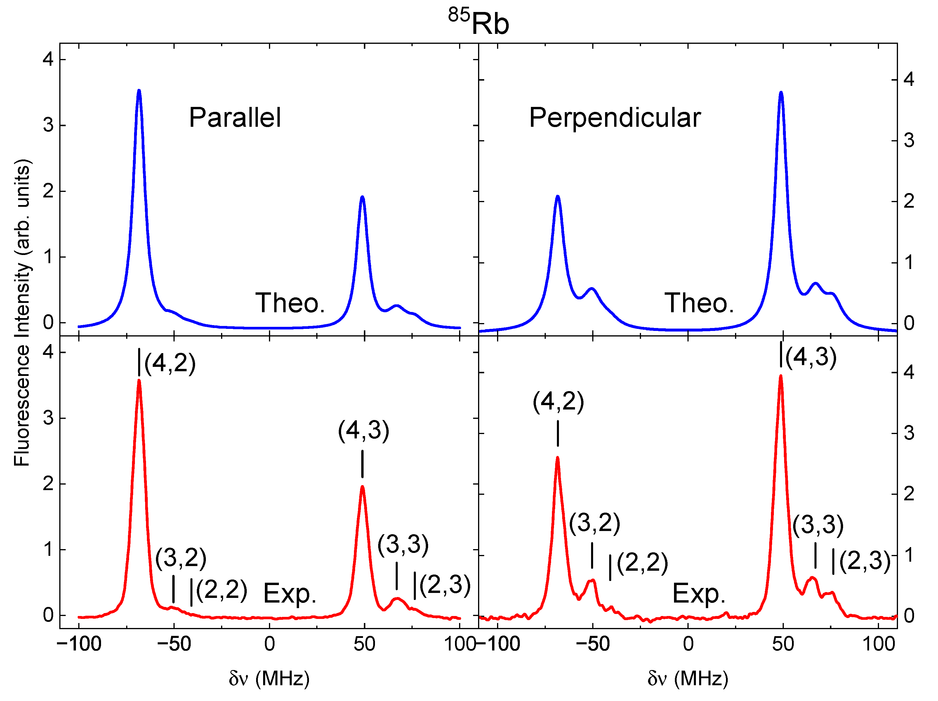
A similar set of spectra, obtained for 85 Rb, is shown in Figure 4. The preparation laser was locked to the F 1 = 3 F 2 = 4 cyclic transition for the group of atoms with a zero-velocity component. The spectra are dominated by the three peaks resulting from the electric quadrupole excitations from this F 2 = 4 hyperfine state into F 3 = 2 , 3 and 4. Once again, satellite lines appear, but now on the high-frequency side of the spectra. In this case, these satellites result from electric quadrupole transitions originating from the F 2 = 3 and 2 hyperfine states into the F 3 = 4 state. The relative intensity of these satellites is not as large, compared to 87 Rb, because for these spectra the power of the preparation laser was about a factor of three larger than the one used for the spectra in Figure 3. The reduction of the relative intensity results from optical pumping of atoms out of the F 2 = 2 and 3 intermediate states [9]. The calculation includes this effect, and therefore produces spectra that are in very good agreement with the experiment.
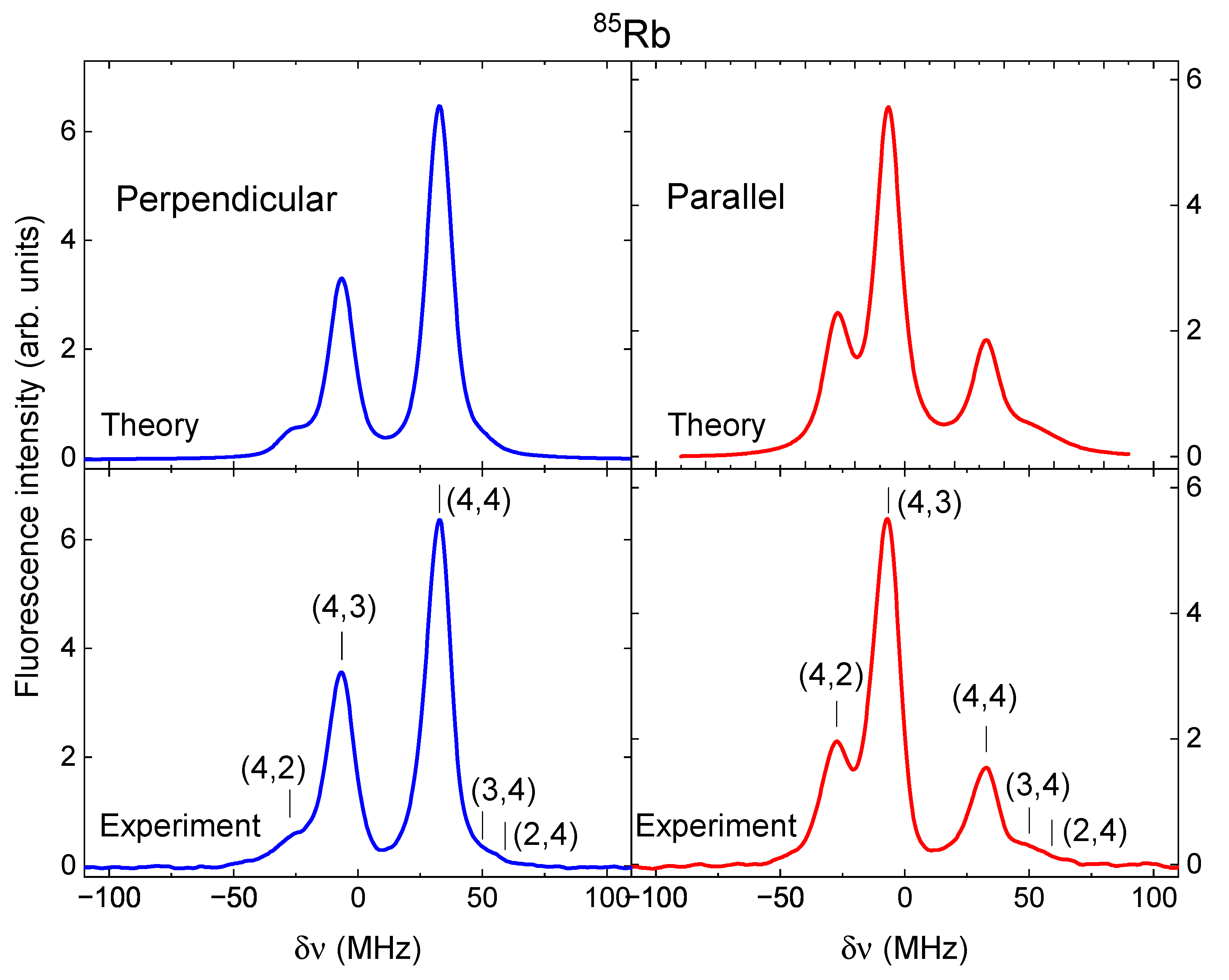
Figure 5 shows spectra for the transition to the other fine structure state of the 6 P manifold in 85 Rb, namely, the 5 P 3 / 2 6 P 1 / 2 electric quadrupole transition [7]. Spectra obtained with parallel and perpendicular polarizations are presented in each panel. Here, the 6 P 1 / 2 hyperfine structure consists of the F 3 = 2 and F 3 = 3 states. One can identify six lines, resulting from electric quadrupole transitions from each of the 5 P 3 / 2 F 2 = 2 , 3 and 4 hyperfine states prepared by selection of velocities. Once again, the main lines result when the preparation step produces the 5 S F 1 = 3 5 P 3 / 2 F 2 = 4 cyclic transition. Sets of two satellite lines appear towards the high-frequency side of these two main lines. The satellites are better resolved in the spectrum with perpendicular polarizations. The results of the velocity-dependent rate equation calculations shown in the top panels [9] are in very good agreement with the experimental data.
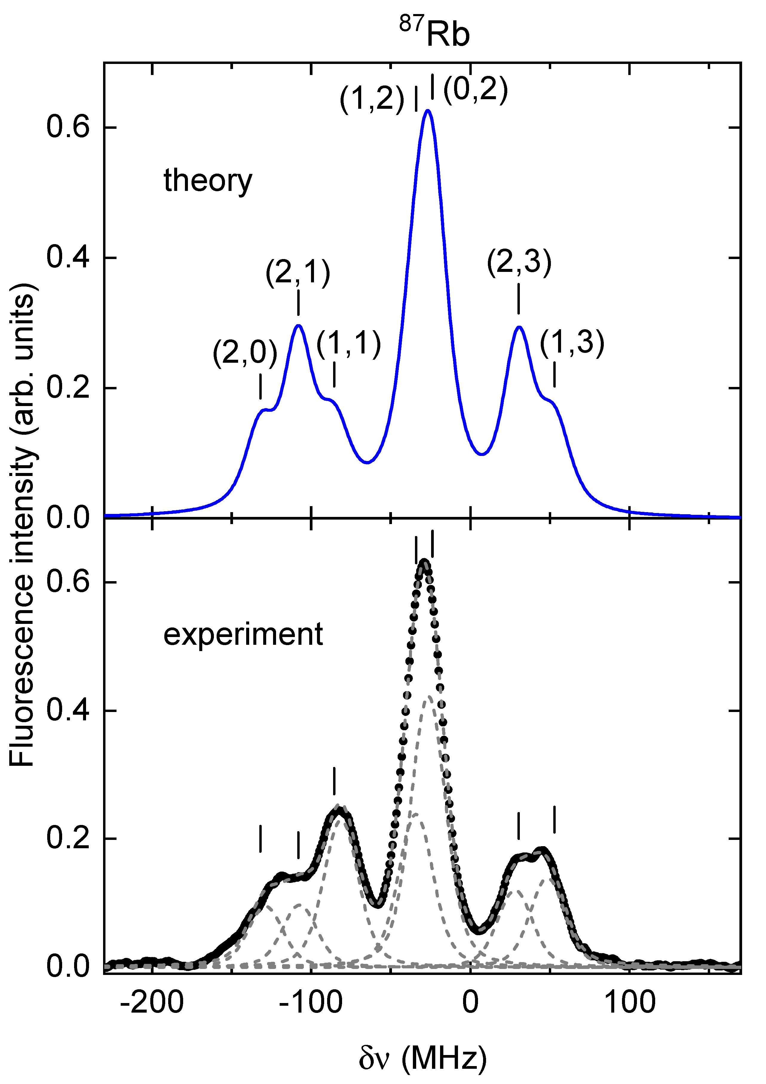
Electric quadrupole transitions can also be observed when the preparation laser is locked to the 5 S F 1 = I 1 / 2 5 P 3 / 2 F 2 = I 3 / 2  low F cyclic transition. A spectrum showing these transitions in 87 Rb is shown in Figure 6 [9]. In this case, there is only one electric quadrupole transition from the 5 P 3 / 2 F 2 = 0 hyperfine state, namely, into the 6 P 3 / 2 F 3 = 2 state. However, the velocity-dependent calculation shows [9] that the preparation laser efficiently populates the other 5 P 3 / 2 F 2 = 1 , 2 states. A fit of Voigt profiles with common widths allows the direct identification of seven lines in the experimental spectrum (bottom panel). The calculation also has seven lines, with the assignment shown in the top panel. In this case, the calculation does not reproduce the relative intensities of all the lines well but does show the presence of three separate groups of transitions. In the first group with three transitions, the experimental results show a stronger ( 1 , 1 ) transition while the calculation indicates that the ( 2 , 1 ) transition should be stronger. Both experiment and theory agree that the group in the center, with ( 1 , 2 ) and ( 0 , 2 ) transitions, should be the one with the largest intensity. Finally, the experimental spectrum has two lines of nearly equal intensity for the third group, and in this case the calculation results in a stronger ( 2 , 3 ) transition. It is important to notice the absence of the ( 2 , 2 ) line in this spectrum, which is forbidden as an electric quadrupole transition.
All 5 P 3 / 2 6 P 3 / 2 electric quadrupole spectra that were studied show a strong dependence on the polarization configuration of both 780 nm and 911 nm lasers [6,7]. The selection rules for electric quadrupole transitions over the magnetic quantum numbers, together with an anisotropic distribution of the populations σ ( F 2 , M 2 ) , are responsible for this behavior. As indicated in Section 4, for relative directions between parallel and perpendicular one expects a P 2 ( cos θ ) dependence on the angle between linear polarizations [6]. Figure 6 of [6] presents a detailed study of the angular distribution of the main line intensities for the 5 P 3 / 2 6 P 3 / 2 forbidden transition in 85 Rb. One can find a similar analysis for the 5 P 3 / 2 6 P 1 / 2 transition in 85 Rb in [7]. The left panel of Figure 7 shows the angular distribution of the intensities of the three main peaks of the 5 P 3 / 2 6 P 3 / 2 transition in 87 Rb. The discrete symbols are the results of the intensities of the F 3 = 1 , 2 and 3 main lines, normalized so that the sum of intensities is equal to one. The dashed lines give the results of fits to functions of the form 4 where ( I 0 , A 0 ) are free parameters. The continuous lines are the results of using the three-step description to calculate I 0 and A 0 . These parameters can be calculated using the populations σ ( F 2 , M 2 ) 
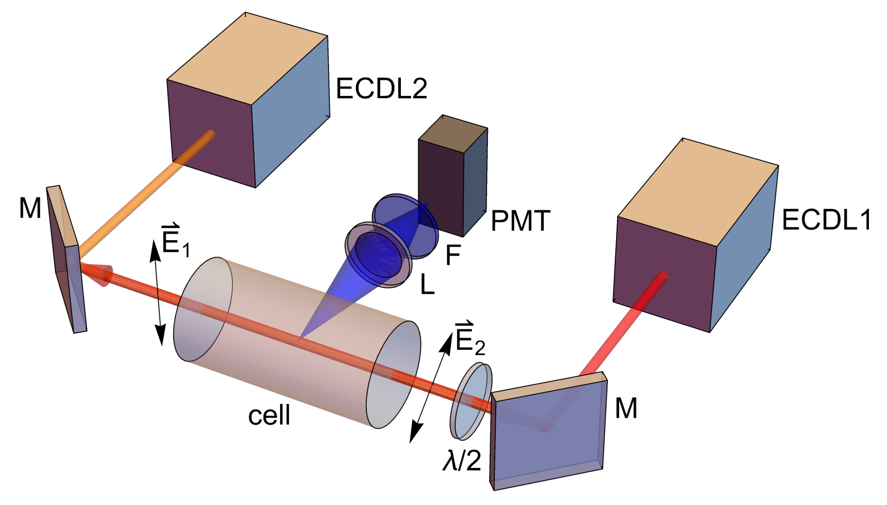
shown in the right-hand panel that were calculated by solving the rate equations. These continuous lines are the result of an ab initio calculation, and therefore contain no free parameters. The small discrepancies between the ab initio calculation and the results of the fits can be explained if one considers imperfections in the degree of polarization of each of the two lasers used in the experiment, and also for the uncertainty in the determination of the zero in the angular scale. The angular dependence was also used to test the theoretical results for the production of the electric quadrupole transition with scalar paraxial Bessel beams, in the sense that no significant difference was found with the angular distribution obtained with a Gaussian beam. In order to excite the electric quadrupole transition with a non-paraxial beam, the experimental setup of Figure 2 has to be modified. The design and implementation of such an experiment are left for future studies.
The electric quadrupole transitions that are reviewed here are seven orders of magnitude weaker than the 5 S 5 P 3 / 2 electric dipole transition. This inherent weakness makes them ideal probes of the Autler–Townes splitting induced by the strong preparation transition. This is studied in detail in [8], where it is shown that a simple three-level model is not adequate to describe the dependence of the Autler–Townes profile intensities on the preparation laser intensity. Velocity distribution effects, when added to the presence of alternative decay routes from the 6 P 3 / 2 state, provided the ingredients needed for an adequate description of the formation of the Autler–Townes doublets [8].
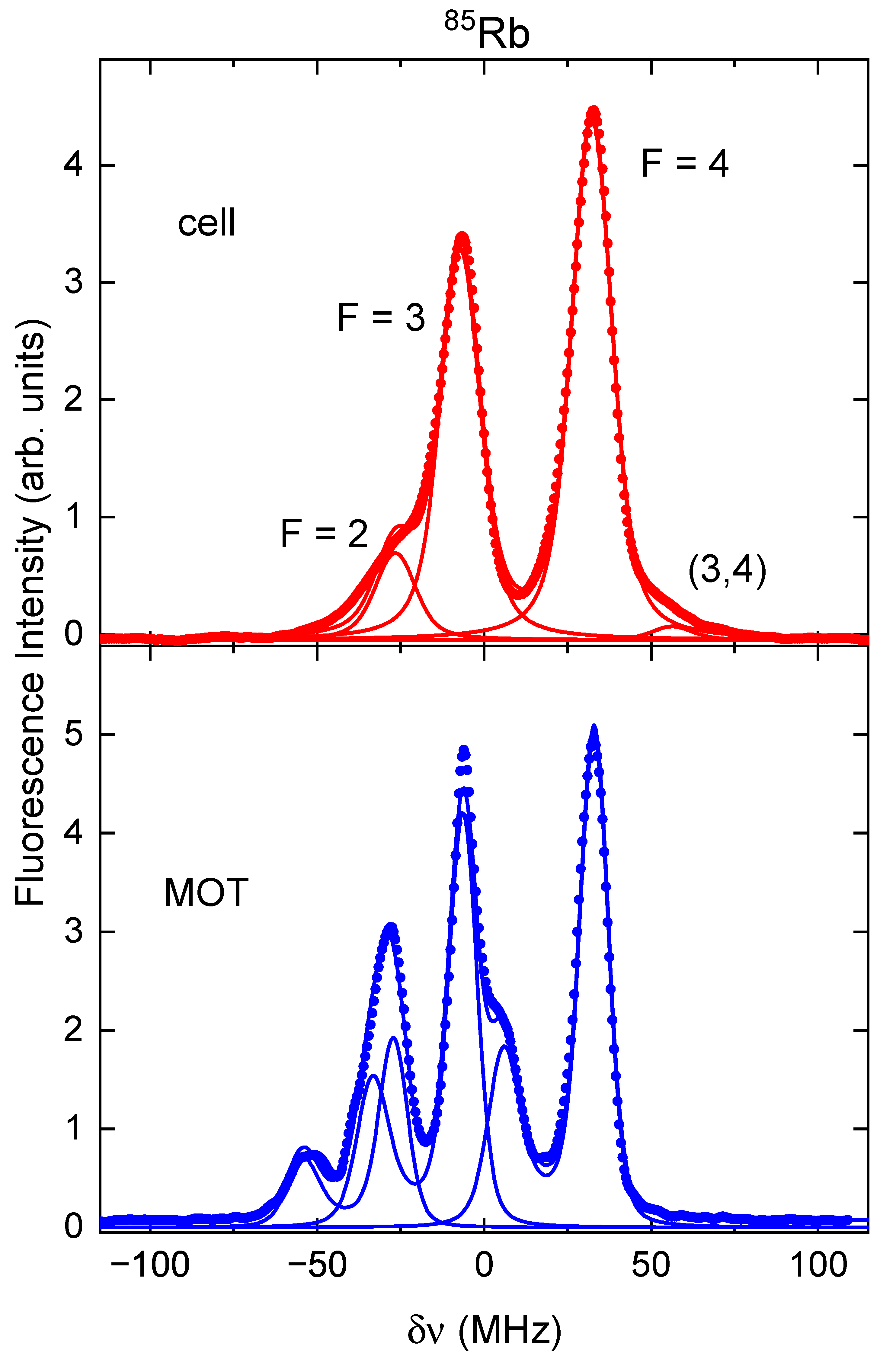
The electric quadrupole transition can also be observed in cold atoms in a magneto-optical trap (MOT) in fully operational conditions. In this case, the MOT trapping and repumping beams are used in the preparation step, and a single 911 nm beam produces the forbidden transition. The intensity of these preparation beams is large enough to produce an Autler–Townes splitting in the fluorescence spectra. Figure 8 shows the comparison between a spectrum recorded in a MOT and that obtained in a cell. These experimental results show the 5 P 3 / 2 6 P 3 / 2 electric quadrupole transition in 85 Rb. For the cell spectrum, the laser intensity is large enough to ensure that the satellite lines do not contribute significantly, but are low enough to stay below the Autler–Townes regime. Furthermore, this cell spectrum was recorded with the linear polarization of the 911 nm laser making an angle of 60 , close enough to the magic angle for which there is no contribution from the coefficient of the angular dependent term in Equation (4). The spectrum obtained with the MOT in the bottom panel shows three sets of asymmetric Autler–Townes doublets, with the strongest component of each doublet aligned with each F 3 transition. It is remarkable that the relative intensities of the three doublets closely resemble the intensity distribution at the magic angle observed in the top panel.
A similar comparison can be made with the 5 P 3 / 2 6 P 3 / 2 electric quadrupole transition for 87 Rb atoms in a MOT and in a cell. Sample spectra showing two stages of the Autler–Townes effect are shown in Figure 9. The comparison is made for commensurate values of the Rabi frequency. These values are obtained directly from the spectra by fitting an Autler–Townes profile to each hyperfine line. The left panels indicate that for a Rabi frequency of about 4 MHz, the Autler–Townes doublet begins to appear. This occurs in both the cell and the MOT. At about twice this value of the Rabi frequency (right panels), the Autler–Townes doublets are clearly defined. The line profiles in the cell (top panel) are symmetric, indicating an effective zero-frequency detuning in the preparation step. The asymmetry in the MOT spectra (bottom panel) is caused by the red detuning of the trapping laser in the MOT. This detuning can be directly obtained from the AT profiles in the spectrum. The relative intensities of the F 3 hyperfine lines in the MOT correspond more to a cell spectrum recorded at the magic angle.

6. Conclusions

This article presented the main results of a study of the 5 P 3 / 2 6 P J ( J = 1 / 2 , 3 / 2 ) electric quadrupole transitions in atomic rubidium. Despite being weak, these transitions can be observed using continuous-wave diode lasers. The use of counterpropagating beams allows recording spectra in which the hyperfine structure of the 6 P J states is completely resolved. When the preparation beam is locked to the large F 1 = I + 1 / 2 F 2 = I + 3 / 2 cyclic transition, the dominant features in the spectra correspond to the electric quadrupole transitions from this maximum F 2 state. Weaker satellite peaks occur because of selection of velocity effects in the preparation step of the transition. A three-step description of the process was proposed, in which a dominant preparation excitation determines the 5 P 3 / 2 F 2 M 2 populations. The description is completed by independently calculating the probabilities associated with the electric quadrupole transition and the direct decay into the ground state by emission of a blue photon. When one includes velocity selection effects in the solution of the rate equations in the preparation step, the results accurately reproduce the behavior of both the main features and the satellite lines. These velocity selection effects are key to understanding the spectrum obtained when the preparation laser frequency is locked to the 5 S F 1 = 1 5 P 3 / 2 F 2 = 0 (low F) cyclic transition in 87 Rb, which has six features in addition to the single F 2 = 0 F 3 = 2 electric quadrupole transition. The relative intensities of all electric quadrupole lines are very sensitive to the relative polarization directions of the laser beams. The theory clearly shows that this dependence results from the F 2 M 2 population distribution in the preparation step, combined with the electric quadrupole selection rules over magnetic quantum numbers. The angular dependence was found to be the same for Gaussian and paraxial scalar Bessel beams. The electric quadrupole transitions are ideal probes of the Autler–Townes effect in both room-temperature and cold atoms. This general understanding of these electric dipole forbidden transitions can be extended to other alkali atoms. The results presented here should be useful in the characterization of atomic samples prepared under a wide variety of conditions.

Author Contributions

Conceptualization, F.R.-M., D.S.S., R.J. and J.J.-M.; setting the experiments and data taking, F.P.-O., C.M.-C., S.H.-G., L.M.H.-C. and J.F.-M.; calculations of the Autler–Townes effect, A.D.A.; writing original draft preparation J.J.-M.; project administration, F.R.-M. and J.J.-M. All authors have read and agreed to the published version of the manuscript.

Funding

This work was supported by DGAPA-UNAM, México, under projects PAPIIT Nos. IN114719 and IN117120, and by Consejo Nacional de Ciencia y Tecnología (CONACyT) and CTIC-UNAM via the Basic Science Grant SEP-CONACyT project No. 285289, and the National Laboratories Program, Grants No. 280181, No. 293471, and No. 299057.

Institutional Review Board Statement

Not applicable.

Informed Consent Statement

Not applicable.

Data Availability Statement

Raw data used to generate all figures are available from the corresponding authors upon reasonable request.

Acknowledgments

We thank J. Rangel for his help in the construction of the diode laser. L.M. Hoyos-Campo thanks UNAM-DGAPA and Conacyt for the postdoctoral fellowship.

Conflicts of Interest

The authors declare no conflict of interest.

References

  1. Chan, E.A.; Aljunid, S.A.; Zheludev, N.I.; Wilkowski, D.; Ducloy, M. Doppler-free approach to optical pumping dynamics in the 6S1/2→5D5/2 electric quadrupole transition of cesium vapor. Opt. Lett. 2016, 41, 2005. [Google Scholar] [CrossRef] [PubMed]
  2. Pucher, S. Spectroscopy of the 6S1/2→5D5/2 Electric Quadrupole Transition of Atomic Cesium. Master’s Thesis, Technischen Universität, Wien, Austria, 2018. [Google Scholar]
  3. Ray, T.; Gupta, R.K.; Gokhroo, V.; Everett, J.L.; Nieddu, T.; Rajasree, K.S.; Chormaic, S.N. Observation of the 87Rb 5S1/2→4D3/2 electric quadrupole transition at 516.6 nm mediated via an optical nanofibre. New J. Phys. 2020, 22, 062001. [Google Scholar] [CrossRef]
  4. Bayram, S.B.; Havey, M.D.; Kupriyanov, D.V.; Sokolov, I.M. Anomalous depolarization of the 5p2P3/2→8p2Pj′ transitions in atomic 87Rb. Phys. Rev. A 2000, 62, 12503. [Google Scholar] [CrossRef]
  5. Ponciano-Ojeda, F.; Hernández-Gómez, S.; López-Hernández, O.; Mojica-Casique, C.; Colín-Rodríguez, R.; Ramírez-Martínez, F.; Flores-Mijangos, J.; Sahagún, D.; Jáuregui, R.; Jiménez-Mier, J. Observation of the 5p3/2→6p3/2 electric-dipole-forbidden transition in atomic rubidium using optical-optical double-resonance spectroscopy. Phys. Rev. A 2015, 92, 042511. [Google Scholar] [CrossRef]
  6. Mojica-Casique, C.; Ponciano-Ojeda, F.; Hernández-Gómez, S.; López-Hernández, O.; Flores-Mijangos, J.; Ramírez-Martínez, F.; Sahagún, D.; Jáuregui, R.; Jiménez-Mier, J. Control of electronic magnetic state population via light polarization in the 5p3/2→6p3/2 electric quadrupole transition in atomic rubidium. J. Phys. B 2017, 20, 025003. [Google Scholar] [CrossRef]
  7. Ponciano-Ojeda, F.; Mojica-Casique, C.; Hernández-Gómez, S.; López-Hernández, O.; Hoyos-Campo, L.; Flores-Mijangos, J.; Ramírez-Martínez, F.; Sahagún, D.; Jáuregui, R.; Jiménez-Mier, J. Optical spectroscopy of the 5p3/2→6p1/2 electric dipole-forbidden transition in atomic rubidium. J. Phys. B 2019, 52, 135001. [Google Scholar] [CrossRef]
  8. Ramírez-Martínez, F.; Ponciano-Ojeda, F.; Hernández-Gómez, S.; Angel, A.D.; Mojica-Casique, C.; Hoyos-Campo, L.M.; Flores-Mijangos, J.; Sahagún, D.; Jáuregui, R.; Jiménez-Mier, J. Electric-dipole forbidden transitions for probing atomic state preparation: The case of the Autler-Townes effect. J. Phys. B 2021, 54, 095002. [Google Scholar] [CrossRef]
  9. Ponciano-Ojeda, F.S.; Mojica-Casique, C.; Hoyos-Campo, L.M.; Ramírez-Martínez, F.; Flores-Mijangos, J.; Jiménez-Mier, J. Study of the velocity-selection satellites present in the 5P3/2→6PJ (J=1/2, 3/2) electric quadrupole transitions in atomic rubidium. J. Phys. B At. Mol. Opt. Phys. 2023, 56, 205002. [Google Scholar] [CrossRef]
  10. Bhattacharya, M.; Haimberger, C.; Bigelow, N. Forbidden Transitions in a Magneto-Optical Trap. Phys. Rev. Lett. 2003, 91, 213004. [Google Scholar] [CrossRef] [PubMed]
  11. Pires, R.; Ascoli, M.; Eyler, E.E.; Gould, P.L. Upper limit on the magnetic dipole contribution to the 5p-8p transition in Rb by use of ultracold atom spectroscopy. Phys. Rev. A 2009, 80, 062502. [Google Scholar] [CrossRef]
  12. Tong, D.; Farooqi, S.; van Kempen, E.; Pavlovic, Z.; Stanojevic, J.; Côté, R.; Eyler, E.; Gould, P. Observation of electric quadrupole transitions to Rydberg nd states of ultracold rubidium atoms. Phys. Rev. A 2009, 79, 052509. [Google Scholar] [CrossRef]
  13. Autler, S.H.; Townes, C.H. Stark Effect in Rapidly Varying Fields. Phys. Rev. 1955, 100, 703. [Google Scholar] [CrossRef]
  14. Metcalf, H.; Van der Straten, P. Laser Cooling and Trapping; Graduate Texts in Contemporary Physics; Springer: Berlin/Heidelberg, Germany, 1999. [Google Scholar]
  15. Glaser, C.; Karlewski, F.; Kluge, J.; Grimmel, J.; Kaiser, M.; Günther, A.; Hattermann, H.; Krutzik, M.; Fortágh, J. Absolute frequency measurement of rubidium 5S-6P transitions. Phys. Rev. A 2020, 102, 012804. [Google Scholar] [CrossRef]
  16. Allegrini, M.; Arimondo, E.; Orozco, L.A. Survey of Hyperfine Structure Measurements in Alkali Atoms. J. Phys. Chem. Ref. Data 2022, 51, 043102. [Google Scholar] [CrossRef]
  17. She, C.Y.; Yu, J.R. Doppler-free saturation fluorescence spectroscopy of Na atoms for atmospheric application. Appl. Opt. 1995, 34, 1063. [Google Scholar] [CrossRef] [PubMed]
  18. Safronova, M.S.; Johnson, W.R.; Derevianko, A. Relativistic many-body calculations of energy levels, hyperfine constants, electric-dipole matrix elements, and static polarizabilities for alkali-metal atoms. Phys. Rev. A 1999, 60, 4476–4487. [Google Scholar] [CrossRef]
  19. Brink, D.; Satchler, G. Angular Momentum, 3rd ed.; Oxford Science Publications, Clarendon Press: Melbourne, Australia, 1993. [Google Scholar]
  20. Sobelman, I. Atomic Spectra and Radiative Transitions, 2nd ed.; Springer Series on Atomic, Optical, and Plasma Physics; Springer: Berlin/Heidelberg, Germany, 1992; Chapter 4; p. 76. [Google Scholar]
  21. Volke-Sepulveda, K.; Garcés-Chávez, V.; Chávez-Cerda, S.; Arlt, J.; Dholakia, K. Orbital angular momentum of a high-order Bessel light beam. J. Opt. B Quantum Semiclass. Opt. 2002, 4, S82–S89. [Google Scholar] [CrossRef]
  22. Durnin, J. Exact solutions for nondiffracting beams. I. The scalar theory. J. Opt. Soc. Am. A 1987, 4, 651–654. [Google Scholar] [CrossRef]
  23. Jáuregui, R. Control of atomic transition rates via laser-light shaping. Phys. Rev. A 2015, 91, 043842. [Google Scholar] [CrossRef]
  24. Schmiegelow, C.T.; Schulz, J.; Kaufmann, H.; Ruster, T.; Poschinger, U.G.; Schmidt-Kaler, F. Transfer of optical orbital angular momentum to a bound electron. Nat. Commun. 2016, 7, 12998. [Google Scholar] [CrossRef] [PubMed]
Figure 1. Energy level diagram of atomic rubidium. (a) Fine structure states that participate in the production of the electric dipole forbidden transition. (b) Representative hyperfine structure of the fine structure states in (a).
Photonics 10 01335 g001
Figure 2. Schematic representation of the setup used for the experiments with room-temperature atoms in an absorption cell. ECDL: external cavity diode laser; M: mirror; L: lens; F: filter; PMT: photomultiplier tube; λ / 2 : half-wave plate.
Photonics 10 01335 g002
Figure 3. Electric quadrupole spectra for the 5 P 3 / 2 6 P 3 / 2 transition in 87 Rb. The left panels are obtained with perpendicular polarizations and the right panels are obtained with parallel polarizations (see text). The top panels are spectra obtained by solving the set of velocity-dependent rate equations.
Photonics 10 01335 g003
Figure 4. Electric quadrupole spectra for the 5 P 3 / 2 6 P 3 / 2 transition in 85 Rb. The left panels are obtained with perpendicular polarizations and the right panels are obtained with parallel polarizations (see text). The top panels are spectra obtained by solving the set of velocity-dependent rate equations.
Photonics 10 01335 g004
Figure 5. Spectra for the 5 P 3 / 2 6 P 1 / 2 electric quadrupole transition in 85 Rb. The left panels are obtained with parallel polarizations and the right panels are obtained with perpendicular polarizations (see text). The top panels are spectra obtained by solving the set of velocity-dependent rate equations.
Photonics 10 01335 g005
Figure 6. Spectra for the low F  5 P 3 / 2 6 P 3 / 2 electric quadrupole transition in 87 Rb. The experimental spectrum is shown in the bottom spectrum, and the results of the calculation with the corresponding line assignment are shown in the top panel.
Photonics 10 01335 g006
Figure 7. Angular distribution of each of the main electric quadrupole lines in 87 Rb. Left panel: the symbols are the result of the normalized intensity of spectra at each angle. The dashed lines are fits of functions of the form I ( θ ) = I 0 1 + A 0 P 2 ( cos θ ) . The continuous lines are the result of the calculated angular distribution using the populations σ ( M 2 ) shown in the right panel.
Photonics 10 01335 g007
Figure 8. Comparison between spectra for 85 Rb recorded in a cell and in an operational magneto-optical trap (MOT).
Photonics 10 01335 g008
Figure 9. Comparison between spectra for 87 Rb recorded in a cell (top panels) and in a magneto-optical trap (MOT) in fully operational conditions (bottom panels).
Photonics 10 01335 g009
Table 1. Squares of the geometric part of the reduced matrix elements for the 5 P 3 / 2 6 P 3 / 2 electric quadrupole transition in both 85 Rb and 87 Rb.
87 Rb
F 2
F 3 0123
000 1 4 0
10 6 25 3 10 21 100
2 1 4 3 10 0 7 10
30 21 100 7 10 21 25
85 Rb
F 2
F 3 1234
1 3 200   7 40   14 25  0
2 7 40   25 56   1 5   3 7  
3 14 25   1 5   21 400   15 16  
40 3 7 15 16 3 4
Table 2. Squares of the geometric part of the reduced matrix elements for the 5 P 3 / 2 6 P 1 / 2 electric quadrupole transition in both 85 Rb and 87 Rb.
87 Rb
F 2
F 3 0123
10 3 40 3 8 21 20
2 1 4 27 40 7 8 7 10
85 Rb
F 2
F 3 1234
2 1 20 1 4   7 10   3 2  
3 7 10 1 21 20 3 4
Disclaimer/Publisher’s Note: The statements, opinions and data contained in all publications are solely those of the individual author(s) and contributor(s) and not of MDPI and/or the editor(s). MDPI and/or the editor(s) disclaim responsibility for any injury to people or property resulting from any ideas, methods, instructions or products referred to in the content.

