Tuning the Photonic Spectrum of Superlattice Structures with Magnetic Fields: An Anisotropic Perspective

Abstract

We investigate how an external magnetic field with an arbitrary direction affects the photonic band of a superlattice structure composed of alternating dielectric and magneto-optical plasma layers. By considering that the superlattice is electrodynamically anisotropic in the presence of an external magnetic field, we derive the dispersion equations; we show that the photonic spectrum of this superlattice loses its degeneracy and splits into two branches due to the external magnetic field. Interestingly, our results indicate that a superlattice that was previously wholly photo-isolating can become entirely photo-conducting, regardless of the direction of the external magnetic field applied. These results could be helpful to design and build new optical diode-like devices.

1. Introduction

In many photonic systems, we commonly focus on the interaction between electromagnetic waves and materials concerning the electric field component. This perspective is biased due to the relatively easy liberation of free electric charges, with magnetic interactions occurring only at a second-order level. Nevertheless, in some cases, because of the high mobility of the free charge carriers in conducting media, their electrodynamic parameters might strongly depend on external magnetic fields. Owing to this, various characteristics of optical devices containing conducting constituents can be altered with the use of an external magnetic field [1,2,3,4,5,6,7,8,9,10,11]. Among various optical systems, optical superlattices, regular structures of alternating layers with different optical parameters, attract great attention. Due to this, it is of interest to analyze how the external magnetic field can alter the photonic characteristics of a superlattice consisting of alternating dielectric and conducting layers. Thus, the study of using magnetic fields in superlattices can be seen as a possible way to design and generate new optical devices for future all-optical technologies. Recently, even the influence of randomness has been studied in similar optical devices [12], and nonlinear modes such as ferroelectric solitons in epitaxial bismuth ferrite superlattices have been successfully observed in experimental setups [13]. In a standard approach, it is assumed that such an external magnetic field points in one constant direction, and then one studies how the strength of this field affects the way that light behaves in the superlattice system. However, in this study, we look at how changing the direction of the external magnetic field can alter the way that the superlattice interacts with light. One notable thing about this work is the consideration of anisotropy. We study the case when the conducting layers of the superlattice become electrodynamically anisotropic in the presence of the external magnetic field. Therefore, the behavior of the conducting layers in the superlattice may change, depending on which way the direction of the external magnetic field is applied. It is well-known how to obtain the photonic spectrum of the isotropic superlattices, which are described in terms of $2\times 2$ unit-cell transfer matrix; see, for example, [14]. As for the anisotropic scenario, the formalism of the $2\times 2$ transfer matrix becomes inapplicable, and it has to be considerably modified. Because of the anisotropy, the dimensions of the unit-cell transfer matrix become $4\times 4$, which considerably complicates the theoretical analysis of the problem [15]. For instance, to describe the eigenstates of the electromagnetic field in the superlattice, one must determine the eigenvalues of the unit-cell transfer matrix. For this, one has to find all roots of an algebraic equation of the fourth degree. In the present study, we show that finding the four roots problem can be reduced to finding the solution of a quadratic equation, whose roots are described by a very well-known formula.

Another critical question is how many new branches in the photonic spectrum of the superlattice can be generated by applying an external magnetic field. On the one hand, as is also well-known, in the absence of the external magnetic field, there is one dispersion relation; for example, ref. [14] shows a degenerated Bloch electromagnetic eigenmode corresponding to propagation of the electromagnetic wave along the axis of the superlattice. On the other hand, the number of eigenstates of the electromagnetic field can be associated with the number of the eigenvalues of the unit-cell transfer matrix, whose value for the $4\times 4$ unit-cell transfer matrix is equal to four. Although the unit-cell transfer matrix generally has four different eigenvalues, it turns out that the photonic spectrum of the superlattice in the presence of the external magnetic field is described by two dispersion equations for two different Bloch phases.

It is worth mentioning that there are, in fact, numerical methods that can be used to simulate the photonic properties of optical systems; see, for instance, [16,17]. It is essential to underline that such numerical algorithms can be applied quite effectively to isotropic optical structures. However, their effectiveness and practicality become significantly limited when it comes to anisotropic systems. Anisotropic materials possess unique properties and behaviors that set them apart from their isotropic counterparts, presenting a distinct challenge for conventional approaches. They have to be modified in a general case where tensors with all non-zero components describe the anisotropy, as takes place in the problem under consideration. The analytical results that we obtain in the present study significantly simplify the problem of describing the photonic properties of the magneto-optical superlattices because we can readily find frequency bands where the superlattice operates as a conductor of electromagnetic waves and where it does as an insulator.

It is worth mentioning that, in paper [18], we studied the impact of the external magnetic field on the propagation of electromagnetic waves in general cases, where both the direction of the wave propagation and the orientation of the magnetic field are arbitrary. To do this, we numerically analyzed the eigenstates of the electromagnetic field within the framework of the transfer matrix method. However, we adopt a pure analytical methodology to unveil the intricate dispersion relations in this current study. These relations are essential in understanding how electromagnetic waves travel through materials with layered structures and distinctive magnetic properties. Our paper is organized as follows: in the next section, we describe the tensorial model used in our anisotropic superlattice system based on classical electromagnetic theory; next, in Section 3, we obtain the corresponding analytical dispersion relations that characterize the photonic spectrum; then, in Section 4, we apply the analytical results for describing a superlattice consisting of dielectric and semiconductor cells, showing the possibility to switch between pure photo-isolating and pure photo-conducting state; finally, in Section 5, we offer the conclusions and point out future work. It is important to remark that, in this work, we are really focusing on just the theoretical aspects. Still, we hope our results can motivate future experimental works to design low-cost anisotropic superlattice photonic systems to control light for future all-optical technologies. In principle, the results obtained here can be used to help build and create an optical diode-like device due to the switching between conducting and non-conducting light in the system.

2. Materials and Methods: Anisotropic Superlattices

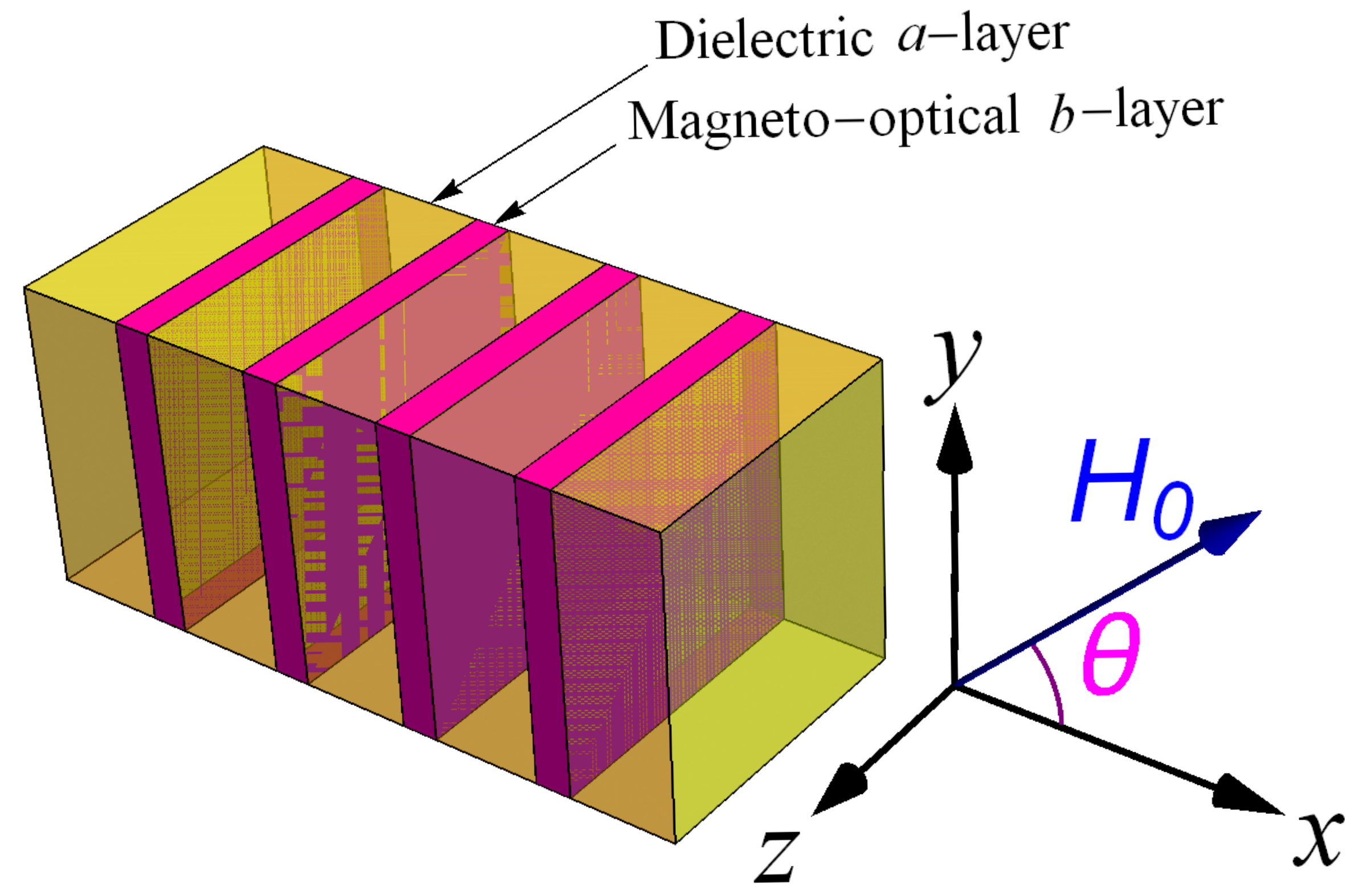
We start by establishing basic relations describing electromagnetic waves propagating along the axis of a superlattice, which is an array composed of identical unit-cells, in the presence of static and homogenous magnetic field ${\mathbf{H}}_0$ of arbitrary direction, as shown in Figure 1. Without loss of generality, we consider that the direction of the magnetic field ${\mathbf{H}}_0$ lies in the x–y plane. The unit-cell contains two layers: the dielectric a-slab and the magneto-optical plasma-containing b-slab, with constant thicknesses $d_a$ and $d_b$, respectively. Below, we assume that the magneto-optical b-slab is a semiconductor and the superlattice is the sequence of the alternating layers of the isolator and semiconductor. The width of each unit $(a,b)$ cell $d=d_a+d_b$ is the spatial period of the superlattice. The dielectric a-slabs are specified by permittivity ${\epsilon }_a$, refractive index $n_a=\sqrt{{\epsilon }_a}$, wave number $k_a=n_a{k}_0$, and phase shift ${\phi }_a=k_a{d}_a$. Quantity $k_0$ is $k_0=\omega /c$, where $\omega$ is the frequency of the electromagnetic wave.

Figure 1. A sketch of the structure. Quantity $\theta$ is the angle between external magnetic field ${\mathbf{H}}_0$ and the x-axis; the direction of the external magnetic field lies in the x–y plane.

In the presence of the external magnetic field ${\mathbf{H}}_0$, the magneto-optical b-slabs are specified by the conductivity tensor $\widehat{\sigma }$. When the direction of the external magnetic field ${\mathbf{H}}_0$ lies in the x–y plane, the conductivity tensor $\widehat{\sigma }$ of the magneto-optical b-layers has the following elements [18]:

$$\begin{array}{ccc}\hfill & & {\sigma }_{xx}=\frac{{\omega }_p^2}{4\pi }\frac{{\omega }_x^2+{(\nu -i\omega )}^2}{\left[{\omega }_c^2+{(\nu -i\omega )}^2\right](\nu -i\omega )},\hfill \end{array}$$

(1)

$$\begin{array}{ccc}& & {\sigma }_{yy}=\frac{{\omega }_p^2}{4\pi }\frac{{\omega }_y^2+{(\nu -i\omega )}^2}{\left[{\omega }_c^2+{(\nu -i\omega )}^2\right](\nu -i\omega )},\hfill \end{array}$$

(2)

$$\begin{array}{ccc}& & {\sigma }_{zz}=\frac{{\omega }_p^2}{4\pi }\frac{\nu -i\omega }{{\omega }_c^2+{(\nu -i\omega )}^2},\hfill \end{array}$$

(3)

$$\begin{array}{ccc}& & {\sigma }_{xy}={\sigma }_{yx}=\frac{{\omega }_p^2}{4\pi }\frac{{\omega }_x{\omega }_y}{\left[{\omega }_c^2+{(\nu -i\omega )}^2\right](\nu -i\omega )},\hfill \end{array}$$

(4)

$$\begin{array}{ccc}& & {\sigma }_{xz}=-{\sigma }_{zx}=\frac{{\omega }_p^2}{4\pi }\frac{{\omega }_y}{{\omega }_c^2+{(\nu -i\omega )}^2},\hfill \end{array}$$

(5)

$$\begin{array}{ccc}& & {\sigma }_{yz}=-{\sigma }_{zy}=-\frac{{\omega }_p^2}{4\pi }\frac{{\omega }_x}{{\omega }_c^2+{(\nu -i\omega )}^2},\hfill \end{array}$$

(6)

where ${\omega }_p=\sqrt{4\pi e^{2}n/m}$ is the plasma frequency, n is the concentration of the charge carriers in the plasma, m is the effective mass of the charge carrier with charge $-e$, ${\omega }_c=\left|e\right|H_0/mc$ is the cyclotron frequency of the charge carrier in the external magnetic field ${\mathbf{H}}_0$, and quantities ${\omega }_x$ and ${\omega }_y$ are ${\omega }_x=e{H}_{0x}/mc$ and ${\omega }_y=e{H}_{0y}/mc$. Expressions in Equations (1)–(6) are obtained within the Drude model. Note that angle $\theta$, which specifies the direction of the external magnetic field, enters the conductivity tensor through the quantities ${\omega }_x$ and ${\omega }_y$:

$${\omega }_x=e{H}_{0}cos\theta /mc,{\omega }_y=e{H}_{0}sin\theta /mc.$$

(7)

The electromagnetic field in the superlattice is a superposition of the static external magnetic field ${\mathbf{H}}_0$, the alternating electric $\mathbf{E}(x,y,z,t)$ field, and the alternating magnetic $\mathbf{H}(x,y,z,t)$ field. Directing the x-axis normally to the layers of the superlattice, the alternating electromagnetic field reads as

$$\begin{array}{c}\hfill \mathbf{E}(x,y,z,t)=\mathbf{E}\left(x\right)exp(-i\omega t),\mathbf{H}(x,y,z,t)=\mathbf{H}\left(x\right)exp(-i\omega t).\end{array}$$

(8)

As follows from the Maxwell equations,

$$\mathrm{curl}\mathbf{E}=i{k}_0\mathbf{H},\mathrm{curl}\mathbf{H}=-i{k}_0{\epsilon }_a\mathbf{E},$$

(9)

inside the dielectric a-layer, while, inside the magneto-optical b-slab,

$$\mathrm{curl}\mathbf{E}=i{k}_0\mathbf{H},\mathrm{curl}\mathbf{H}=-i{k}_0\widehat{\epsilon }\mathbf{E}.$$

(10)

According to the conductivity tensor $\widehat{\sigma }$, we have introduced the permittivity tensor $\widehat{\epsilon }$ of the magneto-optical b-layer in the presence of the external magnetic field:

$${\epsilon }_{\alpha \beta }={\epsilon }_L{\delta }_{\alpha \beta }+\frac{4i\pi }{\omega }{\sigma }_{\alpha \beta },\alpha ,\beta =x,y,z.$$

(11)

Here, quantity ${\epsilon }_L$ is the permittivity of the lattice of the magneto-optical layer.

3. Results: Anisotropic Dispersion Relations

From the anisotropic electromagnetic relations obtained in the past section, we proceed to look for their corresponding analytical dispersion relations. Note that, contrary to the magneto-optical slab, the dielectric layer is isotropic, and the form of the electromagnetic field inside it can be easily established. Thus, inside the dielectric a-layer of the nth unit-cell, the x-dependent part of the electromagnetic field is

$$\begin{array}{ccc}& & E_x^{\left(n\right)}\left(x\right)=0,\hfill \end{array}$$

(12)

$$\begin{array}{ccc}& & E_y^{\left(n\right)}\left(x\right)=A_n^{(-)}exp[-i{k}_a(x-x_{a_n})]+A_n^{(+)}exp\left[i{k}_a(x-x_{a_n})\right],\hfill \end{array}$$

(13)

$$\begin{array}{ccc}& & E_z^{\left(n\right)}\left(x\right)=B_n^{(-)}exp[-i{k}_a(x-x_{a_n})]+B_n^{(+)}exp\left[i{k}_a(x-x_{a_n})\right],\hfill \end{array}$$

(14)

$$\begin{array}{ccc}& & H_x^{\left(n\right)}\left(x\right)=0,\hfill \end{array}$$

(15)

$$\begin{array}{ccc}& & H_y^{\left(n\right)}\left(x\right)=n_a\left\{B_n^{(-)}exp[-i{k}_a(x-x_{a_n})]-B_n^{(+)}exp\left[i{k}_a(x-x_{a_n})\right]\right\},\hfill \end{array}$$

(16)

$$\begin{array}{ccc}& & H_z^{\left(n\right)}\left(x\right)=n_a\left\{-A_n^{(-)}exp[-i{k}_a(x-x_{a_n})]+A_n^{(+)}exp\left[i{k}_a(x-x_{a_n})\right]\right\},\hfill \end{array}$$

(17)

where $x_{a_n}\le x\le x_{b_n}$, and $x_{a_n}$ and $x_{b_n}$ are the coordinates of the left-hand side and right-hand side of the layer, respectively; quantities $A_n^{(-)}$, $A_n^{(+)}$, $B_n^{(-)}$, and $B_n^{(+)}$ are the four complex amplitudes of the electromagnetic field inside the dielectric layer of the nth unit-cell.

The x-dependent part of the electromagnetic field inside the magneto-optical b-slab is a superposition of four modes with four different wave vectors. Thus, inside the magneto-optical b-slab of the nth unit-cell, the components of the electric and magnetic fields are

$$\begin{array}{ccc}& & E_{\alpha }^{\left(n\right)}\left(x\right)=\sum _{s=1}^4{\mathcal{E}}_{\alpha s}{C}_s^{\left(n\right)}exp\left[i{k}_s(x-x_{b_n})\right],\hfill \end{array}$$

(18)

$$\begin{array}{ccc}& & H_{\alpha }^{\left(n\right)}\left(x\right)=\sum _{s=1}^4{\mathcal{H}}_{\alpha s}{C}_s^{\left(n\right)}exp\left[i{k}_s(x-x_{b_n})\right],\hfill \end{array}$$

(19)

where $x_{b_n}\le x\le x_{a_{n+1}}$ and index $\alpha$ can be x, y, or z; $x_{b_n}$ and $x_{a_{n+1}}$ are, respectively, the positions of the left-hand side and right-hand side of the magneto-optical b-layer within the nth unit-cell. The quantities $C_1^{\left(n\right)}$, $C_2^{\left(n\right)}$, $C_3^{\left(n\right)}$, and $C_4^{\left(n\right)}$ in Equations (18) and (19) are the complex amplitudes of the electromagnetic field inside the magneto-optical b-layer of the nth unit-cell; the quantities $k_1$, $k_2$, $k_3$, and $k_4$ are the x-components of the wave vectors of the four electromagnetic modes inside the magneto-optical b-layer.

Let us consider the equations for the electric and magnetic fields within the magneto-optical b-slab. From Equation (10), we obtain that

$$\mathrm{curlcurl}\mathbf{E}=k_0^2\widehat{\epsilon }\mathbf{E},\mathbf{H}=(1/i{k}_0)\mathrm{curl}\mathbf{E}.$$

(20)

The first equation in Equation (20) gives three scalar equations:

$$\begin{array}{ccc}& & E_x\left(x\right)=-\left[{\epsilon }_{xy}{E}_y\left(x\right)+{\epsilon }_{xz}{E}_z\left(x\right)\right]/{\epsilon }_{xx},\hfill \end{array}$$

(21)

$$\begin{array}{ccc}& & E_y^{″}\left(x\right)+k_0^2{\epsilon }_{yx}{E}_x\left(x\right)+k_0^2{\epsilon }_{yy}{E}_y\left(x\right)+k_0^2{\epsilon }_{yz}{E}_z\left(x\right)=0,\hfill \end{array}$$

(22)

$$\begin{array}{ccc}& & E_z^{″}\left(x\right)+k_0^2{\epsilon }_{zx}{E}_x\left(x\right)+k_0^2{\epsilon }_{zy}{E}_y\left(x\right)+k_0^2{\epsilon }_{zz}{E}_z\left(x\right)=0.\hfill \end{array}$$

(23)

Here, the prime means the derivative with respect to x. After substitution of Equation (21) into Equations (22) and (23), we eliminate quantity $E_x\left(x\right)$ and obtain a system of two equations for $E_y\left(x\right)$ and $E_z\left(x\right)$. Such a system can be written as one matrix equation for two-component quantity $E_{\perp }\left(x\right)={(E_y\left(x\right),E_z\left(x\right))}^{\mathrm{T}}$:

$$E_{\perp }^{″}\left(x\right)+k_0^2\widehat{ϵ}{E}_{\perp }\left(x\right)=0,$$

(24)

where elements of 2 × 2 matrix $\widehat{ϵ}$ are related to the components of the permittivity tensor of the magneto-optical b-layer, which is given by Equation (11):

$$\begin{array}{ccc}& & {ϵ}_{11}={\epsilon }_{yy}-{\epsilon }_{xy}{\epsilon }_{yx}/{\epsilon }_{xx},{ϵ}_{12}={\epsilon }_{yz}-{\epsilon }_{xz}{\epsilon }_{yx}/{\epsilon }_{xx},\hfill \\ & & {ϵ}_{21}={\epsilon }_{zy}-{\epsilon }_{xy}{\epsilon }_{zx}/{\epsilon }_{xx},{ϵ}_{22}={\epsilon }_{zz}-{\epsilon }_{xz}{\epsilon }_{zx}/{\epsilon }_{xx}.\hfill \end{array}$$

(25)

It can be checked that ${ϵ}_{21}=-{ϵ}_{12}$.

The matrix equation in Equation (24) has solutions that depend on x as $E_{\perp }\left(x\right)\propto exp\left(ikx\right)$, where k is the x-component of the wave vector within the magneto-optical b-layer. One can see that a general solution of Equation (24) can be formulated in terms of matrix $\widehat{M}\left(k\right)$:

$$\widehat{M}\left(k\right)=k_0^2\widehat{ϵ}-k^2\widehat{I},$$

(26)

where $\widehat{I}$ is the identity matrix. Thus, all possible values of k—$k_1$, $k_2$, $k_3$, and $k_4$—can be determined from the condition $det\widehat{M}\left(k\right)=0$, which leads to a biquadratic equation:

$$k^4-\left({ϵ}_{11}+{ϵ}_{22}\right)k_0^2{k}^2+\left({ϵ}_{11}{ϵ}_{22}+{ϵ}_{12}^2\right)k_0^4=0.$$

(27)

From Equation (27), we obtain the four possible components of the wave vector:

$$k_{1,2}=\mp n_b^{(-)}{k}_0,k_{3,4}=\mp n_b^{(+)}{k}_0,$$

(28)

where the two refractive indexes $n_b^{(-)}$ and $n_b^{(+)}$ of the magneto-optical b-layer are

$$\begin{array}{c}\hfill n_b^{(-)}=\sqrt{\frac{1}{2}\left[{ϵ}_{11}+{ϵ}_{22}-\sqrt{{({ϵ}_{11}-{ϵ}_{22})}^2-4{ϵ}_{12}^2}\right]},\end{array}$$

(29)

$$\begin{array}{c}\hfill n_b^{(+)}=\sqrt{\frac{1}{2}\left[{ϵ}_{11}+{ϵ}_{22}+\sqrt{{({ϵ}_{11}-{ϵ}_{22})}^2-4{ϵ}_{12}^2}\right]}.\end{array}$$

(30)

The quantities ${\mathcal{E}}_{ys}$ and ${\mathcal{E}}_{zs}$, where $s=1,2,3,4$, in the electric field components $E_y\left(x\right)$ and $E_z\left(x\right)$ are the nontrivial solutions of the homogeneous system of equations

$$\left(\begin{array}{cc}{M}_{11}\left(k_s\right)& M_{12}\left(k_s\right)\\ M_{21}\left(k_s\right)& M_{22}\left(k_s\right)\end{array}\right)\left(\begin{array}{c}{\mathcal{E}}_{ys}\\ {\mathcal{E}}_{zs}\end{array}\right)=0,s=1,2,3,4.$$

(31)

The values are easily found. Using them with Equations (21) and (18), we also find the coefficients ${\mathcal{E}}_{xs}$, so that, for quantities ${\mathcal{E}}_{xs}$, ${\mathcal{E}}_{ys}$, and ${\mathcal{E}}_{zs}$, where $s=1,2,3,4$, we have

$$\begin{array}{c}\hfill {\mathcal{E}}_{xs}=\frac{1}{{\epsilon }_{xx}}\left[\frac{M_{11}\left(k_s\right)}{M_{12}\left(k_s\right)}{\epsilon }_{xz}-{\epsilon }_{xy}\right],{\mathcal{E}}_{ys}=1,{\mathcal{E}}_{zs}=-\frac{M_{11}\left(k_s\right)}{M_{12}\left(k_s\right)},s=1,2,3,4.\end{array}$$

(32)

Using the second equation in Equations (20) and Equation (18), one finds that coefficient ${\mathcal{H}}_{xs}$ of the magnetic field is zero, whereas the remaining ones, ${\mathcal{H}}_{ys}$ and ${\mathcal{H}}_{zs}$, are expressed through quantities ${\mathcal{E}}_{zs}$ and ${\mathcal{E}}_{ys}$, respectively:

$$\begin{array}{c}\hfill {\mathcal{H}}_{xs}=0,{\mathcal{H}}_{ys}=-(k_s/k_0){\mathcal{E}}_{zs},{\mathcal{H}}_{zs}=(k_s/k_0){\mathcal{E}}_{ys},s=1,2,3,4.\end{array}$$

(33)

We have obtained the general expressions that completely define the electromagnetic field distribution within the dielectric a- and magneto-optical b-layers. Inside the dielectric layer, the expressions for the components of the electromagnetic field contain four complex amplitudes: $A_n^{(-)}$, $A_n^{(+)}$, $B_n^{(-)}$, and $B_n^{(+)}$. Within the magneto-optical layer, the expressions for the components of the electromagnetic field contain four complex amplitudes as well: $C_1^{\left(n\right)}$, $C_2^{\left(n\right)}$, $C_3^{\left(n\right)}$, and $C_4^{\left(n\right)}$. With the use of the expressions describing the electromagnetic field inside the dielectric a- and magneto-optical b-layers, we can obtain the unit-cell transfer matrix, which describes the wave transmission through the unit-cell of the superlattice. Since, inside the layers of the superlattice, the electromagnetic field is defined by the four amplitudes, the unit-cell transfer matrix has dimensions $4\times 4$.

In the superlattice composed of the a- and b-layers, the complex amplitudes corresponding to the a-layer and those corresponding to the b-layer are not independent; they are related to each other by the continuous boundary conditions for the tangential y- and z-components of the electromagnetic field. Using the boundary conditions at the left ($x=x_{b_n}$) and right ($x=x_{a_{n+1}}$) boundaries of the magneto-optical b-layer within the nth unit-cell, we obtain two matrix relations for quantities $F_n$, $F_{n+1}$, and C:

$$\begin{array}{ccc}& & F_n={\left(A_n^{(+)},A_n^{(-)},B_n^{(+)},B_n^{(-)}\right)}^{\mathrm{T}},\hfill \end{array}$$

(34)

$$\begin{array}{ccc}& & F_{n+1}={\left(A_{n+1}^{(+)},A_{n+1}^{(-)},B_{n+1}^{(+)},B_{n+1}^{(-)}\right)}^{\mathrm{T}},\hfill \end{array}$$

(35)

$$\begin{array}{ccc}& & C={\left(C_n^{\left(1\right)},C_n^{\left(2\right)},C_n^{\left(3\right)},C_n^{\left(4\right)}\right)}^{\mathrm{T}}.\hfill \end{array}$$

(36)

Quantities $F_n$ and $F_{n+1}$ define the state of the electromagnetic field within the dielectric layers of the nth and $(n+1)$th unit-cells, respectively; quantity C defines the state of the electromagnetic field within the magneto-optical b-layer of the nth unit-cell.

One can obtain that the conditions expressing the continuity of the tangential components of the electromagnetic field at the left ($x=x_{b_n}$) and right ($x=x_{a_{n+1}}$) boundaries of the magneto-optical b-layer within the nth unit-cell are

$${\widehat{T}}_a{\widehat{D}}_a{F}_n={\widehat{T}}_{b}C,{\widehat{T}}_b{\widehat{D}}_{b}C={\widehat{T}}_a{F}_{n+1}.$$

(37)

Matrices ${\widehat{T}}_a$, ${\widehat{T}}_b$, ${\widehat{D}}_a$, and ${\widehat{D}}_b$ are given by

$${\widehat{T}}_a=\left(\begin{array}{cccc}1& 1& 0& 0\\ 0& 0& 1& 1\\ 0& 0& -n_a& n_a\\ n_a& -n_a& 0& 0\end{array}\right),{\widehat{T}}_b=\left(\begin{array}{cccc}{\mathcal{E}}_{y1}& {\mathcal{E}}_{y2}& {\mathcal{E}}_{y3}& {\mathcal{E}}_{y4}\\ {\mathcal{E}}_{z1}& {\mathcal{E}}_{z2}& {\mathcal{E}}_{z3}& {\mathcal{E}}_{z4}\\ {\mathcal{H}}_{y1}& {\mathcal{H}}_{y2}& {\mathcal{H}}_{y3}& {\mathcal{H}}_{y4}\\ {\mathcal{H}}_{z1}& {\mathcal{H}}_{z2}& {\mathcal{H}}_{z3}& {\mathcal{H}}_{z4}\end{array}\right),$$

(38)

$$\begin{array}{ccc}\hfill & & {\widehat{D}}_a=\left(\begin{array}{cccc}exp\left(i{\phi }_a\right)& 0& 0& 0\\ 0& exp(-i{\phi }_a)& 0& 0\\ 0& 0& exp\left(i{\phi }_a\right)& 0\\ 0& 0& 0& exp(-i{\phi }_a)\end{array}\right),\hfill \end{array}$$

(39)

$$\begin{array}{ccc}& & {\widehat{D}}_b=\left(\begin{array}{cccc}exp\left(-i{\phi }_b^{(-)}\right)& 0& 0& 0\\ 0& exp\left(i{\phi }_b^{(-)}\right)& 0& 0\\ 0& 0& exp\left(-i{\phi }_b^{(+)}\right)& 0\\ 0& 0& 0& exp\left(i{\phi }_b^{(+)}\right).\end{array}\right).\hfill \end{array}$$

(40)

Here, quantities ${\phi }_b^{(+)}$ and ${\phi }_b^{(-)}$ are

$${\phi }_b^{(\pm )}=k_b^{(\pm )}{d}_b,k_b^{(\pm )}=n_b^{(\pm )}{k}_0.$$

(41)

From Equation (37), we find the following recurrent relation for the complex amplitudes of the electromagnetic field inside the dielectric a-layers of the $(n+1)$th and nth unit-cells:

$$F_{n+1}=\widehat{Q}{F}_n,\widehat{Q}={\widehat{T}}_a^{-1}{\widehat{T}}_b{\widehat{D}}_b{\widehat{T}}_b^{-1}{\widehat{T}}_a{\widehat{D}}_a.$$

(42)

Matrix $\widehat{Q}$ has the meaning of the unit-cell transfer matrix since it describes the wave transmission through the entire $(a,b)$ unit-cell.

To obtain the dispersion relations describing the eigenstates of the electromagnetic field, we have to find the eigenvalues of the unit-cell transfer matrix $\widehat{Q}$. They can be determined from algebraic equation $det(\widehat{Q}-\lambda \widehat{I})=0$ for unknown quantity $\lambda$, where $\widehat{I}$ is the identical matrix. Since the dimensions of the unit-cell transfer matrix $\widehat{Q}$ are $4\times 4$, it has the four eigenvalues ${\lambda }_1$, ${\lambda }_2$, ${\lambda }_3$, and ${\lambda }_4$, satisfying a polynomial equation of the fourth degree

$$det(\widehat{Q}-\lambda \widehat{I})=0\to {\lambda }^4+u{\lambda }^3+r{\lambda }^2+u\lambda +1=0,$$

(43)

Coefficients u and r are expressed through the parameters of the problem as follows:

$$\begin{array}{c}u=\left[M_{-}sin\left({\phi }_b^{(-)}\right)+M_{+}sin\left({\phi }_b^{(+)}\right)\right]sin\left({\phi }_a\right)\hfill \\ -2cos\left({\phi }_a\right)\left[cos\left({\phi }_b^{(-)}\right)+cos\left({\phi }_b^{(+)}\right)\right],\hfill \end{array}$$

(44)

$$\begin{array}{c}r=2+2cos\left({\phi }_b^{(-)}\right)cos\left({\phi }_b^{(+)}\right)\left[1+cos\left(2{\phi }_a\right)\right]\hfill \\ -\left[M_{-}sin\left({\phi }_b^{(-)}\right)cos\left({\phi }_b^{(+)}\right)+M_{+}cos\left({\phi }_b^{(-)}\right)sin\left({\phi }_b^{(+)}\right)\right]sin\left(2{\phi }_a\right)\hfill \\ +M_{-}{M}_{+}sin\left({\phi }_b^{(-)}\right)sin\left({\phi }_b^{(+)}\right){sin}^2\left({\phi }_a\right).\hfill \end{array}$$

(45)

Here, quantities $M_{\mp }$ are given by

$$M_{-}=\frac{n_a}{n_b^{(-)}}+\frac{n_b^{(-)}}{n_a},M_{+}=\frac{n_a}{n_b^{(+)}}+\frac{n_b^{(+)}}{n_a}.$$

(46)

As a main result of our derivation, it is important to note that, due to the symmetry of the coefficients in the quartic equation in Equation (43), the problem can be reduced to a pure quadratic equation $w^2+uw+r-2=0$ by means of the following change in variables: $\lambda +{\lambda }^{-1}=w$. As a result, the roots ${\lambda }_1$, ${\lambda }_2$, ${\lambda }_3$, and ${\lambda }_4$ of Equation (43) are

$$\begin{array}{ccc}\hfill & & {\lambda }_{1,2}=\frac{1}{4}\left[-u-\sqrt{D}\pm \sqrt{{\left(-u-\sqrt{D}\right)}^2-16}\right],\hfill \end{array}$$

(47)

$$\begin{array}{ccc}& & {\lambda }_{3,4}=\frac{1}{4}\left[-u+\sqrt{D}\pm \sqrt{{\left(-u+\sqrt{D}\right)}^2-16}\right],\hfill \end{array}$$

(48)

$$\begin{array}{ccc}& & D=u^2-4r+8.\hfill \end{array}$$

(49)

From Equations (47) and (48), one can see that only two out of four eigenvalues are independent, since

$${\lambda }_1{\lambda }_2=1,{\lambda }_3{\lambda }_4=1.$$

(50)

Therefore, if, for the independent eigenvalues, we choose ${\lambda }_1$ and ${\lambda }_3$, then the remaining two, ${\lambda }_2$ and ${\lambda }_4$, are expressed through ${\lambda }_1$ and ${\lambda }_3$, respectively:

$${\lambda }_2=1/{\lambda }_1,{\lambda }_4=1/{\lambda }_3.$$

(51)

Owing to Equation (51), we can express the four eigenvalues ${\lambda }_1$, ${\lambda }_2$, ${\lambda }_3$, and ${\lambda }_4$ of the unit-cell transfer matrix through two independent quantities ${\gamma }_{+}$ and ${\gamma }_{-}$:

$$\begin{array}{ccc}\hfill & & {\lambda }_1=exp\left(i{\gamma }_{+}\right),{\lambda }_2=exp\left(-i{\gamma }_{+}\right),\hfill \end{array}$$

(52)

$$\begin{array}{ccc}& & {\lambda }_3=exp\left(i{\gamma }_{-}\right),{\lambda }_4=exp\left(-i{\gamma }_{-}\right).\hfill \end{array}$$

(53)

Here, ${\gamma }_{+}$ and ${\gamma }_{-}$ are the Bloch phases of the electromagnetic eigenmodes of the superlattice in the presence of the external magnetic field. From these equations, one can see that the two Bloch phases ${\gamma }_{+}$ and ${\gamma }_{-}$ satisfy the relations

$$\begin{array}{c}\hfill cos\left({\gamma }_{+}\right)=\left({\lambda }_1+{\lambda }_2\right)/2,cos\left({\gamma }_{-}\right)=\left({\lambda }_3+{\lambda }_4\right)/2,\end{array}$$

(54)

or, equivalently,

$$cos\left({\gamma }_{+}\right)=\left(-u-\sqrt{D}\right)/4,cos\left({\gamma }_{-}\right)=\left(-u+\sqrt{D}\right)/4.$$

(55)

After substitution of Equations (44), (45), and (49) into Equation (55), one finds the equations for the Bloch phases ${\gamma }_{\pm }$. Such a form of the equations is not final, and they can be simplified: after some algebra, one can obtain that quantity $D=u^2-4r+8$ can be represented as a perfect square:

$$\begin{array}{ccc}\hfill & & D=\{2\left[cos\left({\phi }_b^{(-)}\right)-cos\left({\phi }_b^{(+)}\right)\right]cos\left({\phi }_a\right)+[M_{+}sin\left({\phi }_b^{(+)}\right)\hfill \\ & & -M_{-}sin\left({\phi }_b^{(-)}\right)]sin\left({\phi }_a\right){\}}^2.\hfill \end{array}$$

(56)

This allows us to remove the irrationality $\sqrt{D}$ in Equation (55); one can use the expression in the curly brackets in Equation (56) as $\sqrt{D}$. Then, substituting Equation (44) into Equation (55), we obtain the final form of the desired dispersion equations:

$$\begin{array}{ccc}& & cos\left({\gamma }_{-}\right)=cos\left({\phi }_a\right)cos\left({\phi }_b^{(-)}\right)-\frac{1}{2}{M}_{-}sin\left({\phi }_a\right)sin\left({\phi }_b^{(-)}\right),\hfill \end{array}$$

(57)

$$\begin{array}{ccc}& & cos\left({\gamma }_{+}\right)=cos\left({\phi }_a\right)cos\left({\phi }_b^{(+)}\right)-\frac{1}{2}{M}_{+}sin\left({\phi }_a\right)sin\left({\phi }_b^{(+)}\right).\hfill \end{array}$$

(58)

Remarkably, we have obtained the following essential result: we find that, in the presence of the external magnetic field, the photonic spectrum of the superlattice is, therefore, characterized by two dispersion relations for two Bloch modes: ${\gamma }_{+}$ and ${\gamma }_{-}$. This result, considering anisotropy, is contrary to the case of the isotropic superlattice, where only one Bloch mode can exist.

It is not difficult to check that, in the limit of the vanishing external magnetic field $H_0\to 0$, the Bloch phases ${\gamma }_{-}$ and ${\gamma }_{+}$ go to the Bloch phase $\gamma$ of the isotropic superlattice

$${\gamma }_{-}\left(\omega \right)\to \gamma \left(\omega \right),{\gamma }_{+}\left(\omega \right)\to \gamma \left(\omega \right)\mathrm{as}{H}_0\to 0.$$

(59)

Indeed, in the absence of the external magnetic field, the refractive indexes $n_b^{(-)}$ and $n_b^{(+)}$ of the magneto-optical b-layer become equal to each other:

$$n_b^{(-)}=n_b^{(+)}=n_b=\sqrt{{\epsilon }_b}\mathrm{when}{H}_0=0,$$

(60)

where

$${\epsilon }_b={\epsilon }_L-{\omega }_p^2/\omega (\omega +i\nu )$$

(61)

is the Drude permittivity of the magneto-optical b-layer. Due to this,

$$M_{-}=M_{+}=\frac{n_a}{n_b}+\frac{n_b}{n_a}\mathrm{and}{\phi }_b^{(-)}={\phi }_b^{(+)}={\phi }_b=n_b{k}_0{d}_b\mathrm{when}{H}_0=0.$$

(62)

Consequently, as follows from Equations (57) and (58), when the value of the external magnetic field decreases, the photonic spectrums ${\gamma }_{-}={\gamma }_{-}\left(\omega \right)$ and ${\gamma }_{+}={\gamma }_{+}\left(\omega \right)$ merge into one $\gamma =\gamma \left(\omega \right)$, which satisfies the dispersion equation

$$\begin{array}{c}\hfill cos\left(\gamma \right)=cos\left({\phi }_a\right)cos\left({\phi }_b\right)-\frac{1}{2}\left(\frac{n_a}{n_b}+\frac{n_b}{n_a}\right)sin\left({\phi }_a\right)sin\left({\phi }_b\right),H_0=0,\end{array}$$

(63)

where ${\phi }_a=n_a{k}_0{d}_a$ and ${\phi }_b=n_b{k}_0{d}_b$. This is a well-known dispersion equation [14] that describes propagation of the electromagnetic waves in the superlattice composed of the isotropic a- and b-slabs with refractive indexes $n_a=\sqrt{{\epsilon }_a}$ and $n_b=\sqrt{{\epsilon }_b}$, respectively. Therefore, the equations of the photonic spectrums obtained in this work, considering anisotropy, can be considered as a generalization of the pure isotropic scenario.

4. Discussion: The Anisotropic Superlattice

Next, we apply the analytical results obtained in the preceding sections to a superlattice consisting of the dielectric and semiconductor slabs. We consider the following physical and representative parameters: the dielectric a-slab is made of quartz with a refractive index $n_a=2$ (see paper [19]), while the semiconductor b-slab is made of indium antimonide, with concentration of the charge carriers $n={10}^{15}$ cm ${}^{-3}$ and permittivity of the lattice ${\epsilon }_L=17.8$. Additionally, for simplicity, we assume that there is no absorption in the layers of the superlattice, so that the relaxation frequency $\nu$ in the plasma of b-layers can be set to zero:

$$\nu =0.$$

(64)

The thicknesses of the dielectric a- and semiconductor b-layers are $d_a=20\times \delta$ and $d_b=0.5\times \delta$, where $\delta =c/{\omega }_p$ and ${\omega }_p=\sqrt{4\pi n{e}^2/m}$. The numerical values of the quantities listed above are ${\omega }_p/2\pi \approx 2.3$ THz, $\delta \approx 0.02$ mm, $d_a\approx 0.4$ mm, and $d_b\approx 0.01$ mm.

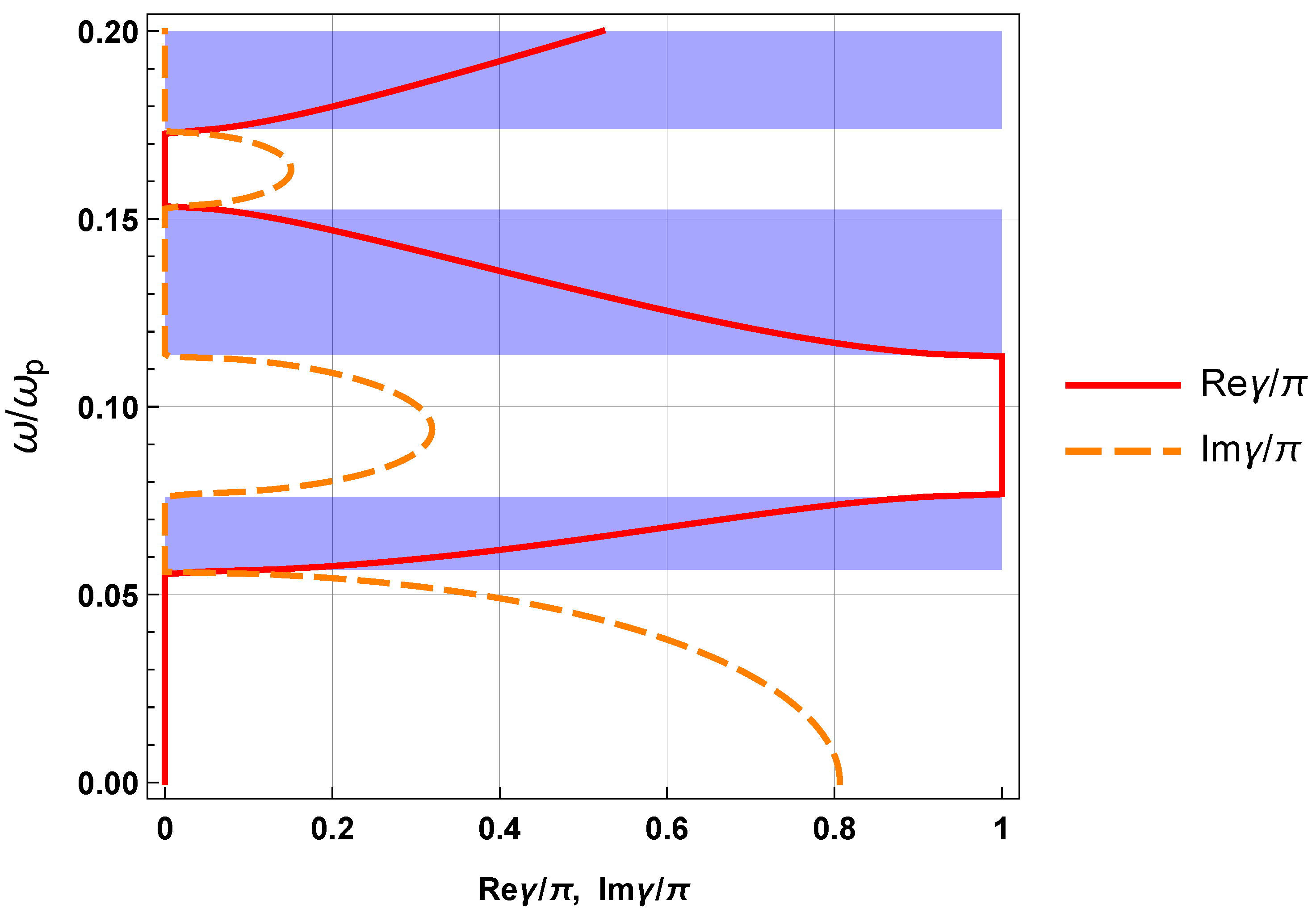
Figure 2 displays the photonic spectrum of the superlattice in the absence of the external magnetic field, $H_0=0$, within frequency range $0\le \omega \le 0.2\times {\omega }_p$. The passbands are highlighted in blue, while the spectral gaps are displayed in white.

Figure 2. Photonic spectrum of the superlattice in the absence of the external magnetic field, $H_0=0$.

Below we consider a frequency region located inside the first lower photonic stop band, beneath frequency $0.05\times {\omega }_p/2\pi \approx 0.116\mathrm{THz}$, where, in the absence of the external magnetic field, $H_0=0$, the superlattice cannot conduct light since there are no propagating states of the electromagnetic field within region $0\le \omega \le 0.05\times {\omega }_p$ (see Figure 2). 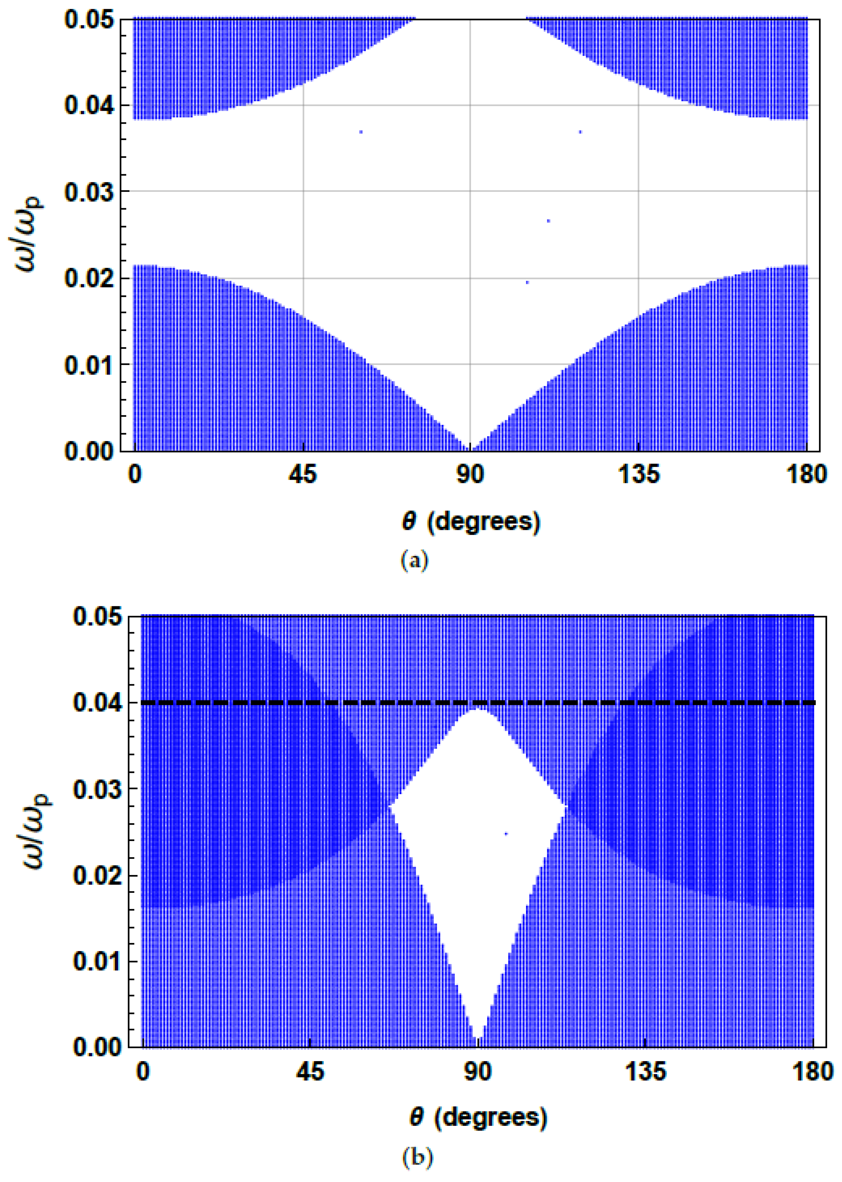Note that frequency $0.05\times {\omega }_p/2\pi \approx 0.116\mathrm{THz}$ corresponds to wavelength of 0.26 $\mathrm{cm}$ in vacuum. Next, we show how the photonic band structure of the superlattice changes in the presence of the external magnetic field of magnitudes $H_0=0.1$ T and $H_0=0.4$ T, within the frequency range $0\le \omega \le 0.05\times {\omega }_p$ and for angles of the external magnetic field within the region $0^{\circ }\le \theta \le {180}^{\circ }$. Angle $\theta$ defines the direction of the external magnetic field ${\mathbf{H}}_0$ relatively to the x-axis; the direction of the external magnetic field ${\mathbf{H}}_0$ lies in the x–y plane.

In the absence of absorption, the two refractive indexes $n_b^{(\mp )}$ of the b-layer are either pure imaginary or pure real. Therefore, the right-hand sides of the dispersion equations in Equations (57) and (58) are real. Therefore, within some frequency bands where

$$|cos\left({\gamma }_{-}\right)|\le 1\mathrm{or}|cos\left({\gamma }_{+}\right)|\le 1,$$

(65)

there are pure real solutions for the Bloch phase ${\gamma }_{-}$ or for the Bloch phase ${\gamma }_{+}$. It is apparent that such solutions with real ${\gamma }_{-}$ or ${\gamma }_{+}$ define the photonic pass bands where the propagating states of the electromagnetic field exist.

Figure 3a shows the photonic band structure when the strength of the external magnetic field is 0.1 T. The white area corresponds to the points $(\theta ,\omega )$ where there are no propagating states of the electromagnetic field. At such values of angle $\theta$ and frequency $\omega$, the superlattice cannot conduct light. The blue area displays points $(\theta ,\omega )$ where the propagating states of the electromagnetic field exist, i.e., where the superlattice can conduct light. It is pretty remarkable that the external magnetic field results in the existence of the propagating states of the electromagnetic field within the photonic stop band of the superlattice in the absence of the external magnetic field. Thus, this result reported here could be helpful in designing and generating optical diode-like devices. A distinctive feature of the band structure shown in Figure 3a is that the size of the photonic pass band strongly depends on the direction $\theta$ of the external magnetic field. Indeed, as one can see, the size of the lower photonic pass band varies from approximately $0.02\times {\omega }_p$ at $\theta =0^{\circ }$ to zero at $\theta ={90}^{\circ }$. The size of the next photonic pass band strongly depends on the angle $\theta$ too.

Figure 3. Photonic band structure of the superlattice for two values of the strength $H_0$ of the external magnetic field: $H_0=0.1$ T (a) and $H_0=0.4$ T (b).

Figure 3b displays the photonic band structure when the strength of the external magnetic field is 0.4 T. Unlike the previous figure, one can see the region from the frequency which approximately equals $0.04\times {\omega }_p$ (the black horizontal dashed line) to the frequency $0.05\times {\omega }_p$, which is completely filled with the propagating states of the electromagnetic field, regardless of the direction $\theta$ of the external magnetic field. Therefore, and remarkably, we found that at any orientation $\theta$ of the external magnetic field, the superlattice can conduct light, providing that the magnetic field is apparently strong enough.

5. Conclusions

In summary, we have examined the impact of the external magnetic field’s direction on the superlattice’s photonic spectrum, composed of alternating dielectric and magneto-optical plasma-containing layers, by considering anisotropy. We have successfully solved this problem using analytical methods, obtaining dispersion equations that describe the propagation of electromagnetic waves in the superlattice in the case of the arbitrary direction of the external magnetic field. Our results show that the photonic spectrum of the superlattice changes significantly when the external magnetic field is applied, giving rise to two distinct branches in the photonic spectrum of the superlattice. Interestingly, the magnetic field induces the propagating states within the superlattice’s photonic stop band, where the electromagnetic field’s propagating modes are typically forbidden. Consequently, there is a transition from a photo-isolating state to a photo-conducting one, which depends on the strength and direction of the external magnetic field. Moreover, the size of the photonic pass band is found to be heavily influenced by the direction of the external magnetic field. However, we have also discovered that, at specific magnetic field strengths, the superlattice undergoes a complete transition from a photo-isolating to a photo-conducting state, where the propagating states of the electromagnetic field are observed inside the photonic stop band, regardless of the direction of the external magnetic field. Future research work could comprehensively characterize the photonic band structure in superlattices, potentially exploring more intricate designs and accounting for nonlinear effects. We hope the findings presented in this study may serve as a valuable foundation for developing future photonic devices, carefully considering their unique anisotropic properties.